Improved algorithms and methods for room sound-field prediction by acoustical radiosity in arbitrary polyhedral rooms Eva-Marie Nosala) Department of Mathematics, University of British Columbia, Vancouver, BC, Canada V6T 1Z2
Murray Hodgson School of Occupational and Environmental Hygiene and Department of Mechanical Engineering, University of British Columbia, Vancouver, BC, Canada V6T 1Z3
Ian Ashdown by Heart Consultants Limited, West Vancouver, BC, Canada V7S 1W3
共Received 30 March 2003; revised 6 March 2004; accepted 20 May 2004兲 This paper explores acoustical 共or time-dependent兲 radiosity—a geometrical-acoustics sound-field prediction method that assumes diffuse surface reflection. The literature of acoustical radiosity is briefly reviewed and the advantages and disadvantages of the method are discussed. A discrete form of the integral equation that results from meshing the enclosure boundaries into patches is presented and used in a discrete-time algorithm. Furthermore, an averaging technique is used to reduce computational requirements. To generalize to nonrectangular rooms, a spherical-triangle method is proposed as a means of evaluating the integrals over solid angles that appear in the discrete form of the integral equation. The evaluation of form factors, which also appear in the numerical solution, is discussed for rectangular and nonrectangular rooms. This algorithm and associated methods are validated by comparison of the steady-state predictions for a spherical enclosure to analytical solutions. © 2004 Acoustical Society of America. 关DOI: 10.1121/1.1772400兴 PACS numbers: 43.55.Ka, 43.55.Br 关MK兴
I. INTRODUCTION
Room acousticians have been attempting to understand and predict the behavior of sound in rooms for hundreds of years. The prediction of sound fields in enclosures is needed for design purposes, such as the optimization of classrooms and lecture halls for intelligibility, of concert halls, recording studios, and theatres for sound quality, of workrooms for minimized noise levels, of offices for privacy, and so on. Moreover, as computer simulations become increasingly popular for entertainment and training purposes, fast and accurate room-acoustical modeling techniques are required. One approach to room acoustics is through geometricalacoustics models, in which sound waves are replaced by sound rays.1,2 As many important perceptual effects mainly involve middle to high frequencies 共where geometricalacoustics models are accurate兲 such models have been used extensively in room acoustics over the past 40 years. This paper explores a geometrical-acoustics method known as acoustical radiosity 共AR兲. The method assumes perfectly lambertian-diffuse reflection from all surfaces of the enclosure. AR has been called various names, including the integral equation method,2 radiant exchange,3 and an intensitybased boundary element method.4 The name ‘‘acoustical radiosity’’ is taken from a similar 共time-independent兲 technique used in computer graphics, where it is simply called radiosity.5–7 a兲
Author to whom correspondence should be addressed. Current affiliation: School of Ocean and Earth Sciences and Technology, Department of Geology and Geophysics, University of Hawaii at Manoa, 1680 East-West Road POST 813, Honolulu, HI, 96822; Electronic mail:
[email protected]
970
J. Acoust. Soc. Am. 116 (2), August 2004
Pages: 970–980
Kuttruff derived the governing integral equation for AR in the early 1970s.2,8,9 Analytical solutions for the integral equation exist for spheres10–13 and for infinitely long, flat enclosures2,14 共in which side walls are neglected兲. In general, however, the equation must be solved numerically. Several papers outline and/or make use of a numerical solution to the integral equation. In 1984, Miles15 gave a detailed account of his iterative solution for both steady-state and time-varying sources in rectangular enclosures. In 1993, Lewers3 used AR to model the diffuse reverberant tail of the impulse response in a hybrid model. Shi, Zhang, Encarnac¸˜ao, and Go¨bel,16 outlined an algorithm for AR, but few details or results were given. More recently, Le Bot and Bocquillet,17 compared steady-state sound-level predictions from AR to predictions from ray tracing, and Kang18 used AR to investigate the propagation of sound in long enclosures with diffusely reflecting boundaries. Despite these developments and the potential of AR, relatively little attention has been given to the technique. Reasons for this likely include the limiting assumption of diffuse reflection and high computational costs. As discussed in this paper, neither assumption is unreasonably restrictive—AR deserves further attention. In particular, there is a need for a clear, complete exposition of the theory and assumptions behind the method. Moreover, algorithms and methods nonrectangular rooms need to be further developed for and incorporated into AR. These should include improvements for efficiency, and the numerical solution should be validated. These aspects are the objectives of the present paper.
0001-4966/2004/116(2)/970/11/$20.00
© 2004 Acoustical Society of America
II. ASSUMPTIONS, DISADVANTAGES, AND BENEFITS OF ACOUSTICAL RADIOSITY
Since AR is an energy-based method, phase relationships between propagating waves are assumed incoherent.13 This assumption is usually sufficient, and may be justified when the wavelengths are small compared to the dimensions of the room.19 Further simplifications made in this work include reflection coefficients independent of their angle of incidence, empty convex enclosures, and omni-directional point sources. The main assumption of AR is that all boundaries are diffusely reflecting—that is, reflection is governed by Lambert’s law, I 共 ,R 兲 ⫽I 共 0,R 兲 cos ,
共1兲
where I( ,R) is the intensity of the sound which is scattered by a surface element in direction 共0⭐⭐/2兲 from the surface normal measured at distance R from the element 共this formulation is different from in other fields, such as computer graphics, because of the differences in definition of intensity兲. This assumption allows for major simplifications in the development of the model because diffuse reflection is memoryless. In particular, the way that a ray is reflected is not dependent on the direction from whence it came. It has been suggested13,20 that the assumption of diffuse reflection is less restrictive than the commonly made assumption of specular reflection, and it is certainly less restrictive than the assumption of a diffuse field that is still popular among room acousticians. Further, some characteristics of the field may not be sensitive to a change from specular to diffuse reflection.21,22 AR may be an effective predictor of such characteristics. Certainly, it is likely that AR is highly effective in predicting the late part of a decay curve. It has been shown that the conversion of specular energy into diffuse energy is irreversible and that all walls produce some diffuse reflection.23 Hence, though the initial reflections in a room may be more specular than diffuse, most of the energy in the sound decay of a room will involve higher-order, diffuse reflections. Indeed, after several reflections, nearly all energy becomes diffusely reflecting.20 The effectiveness of AR in predicting the late part of decay curves has been shown for spherical12 and rectangular23 enclosures by comparison of decay curves for rooms with and without diffusely reflecting walls. Thus, hybrid methods that account for the specular component by another method 共such as ray-tracing or the method of images兲 and for the diffuse component by AR may be highly successful in predicting room sound fields. Such a model was suggested by Lewers3 and, for rectangular enclosures, by Baines.24 It may be possible to extend AR methods to nondiffuse reflection. Such extensions have been made in computer graphics for time-independent cases25–27 and for a few timedependent cases.28,29 Time dependence in AR is one of its limitations, because of the high computational costs involved 共in other fields, such as computer graphics, radiosity is time independent兲. Nevertheless, the method is promising, since the costs are J. Acoust. Soc. Am., Vol. 116, No. 2, August 2004
FIG. 1. Geometry relevant to the integral equation.
incurred only in the initial rendering of a room. In particular, once a room has been rendered for a given source, the remaining computational costs are low enough to enable realtime sound-field simulation for moving receivers. This view independence is particularly advantageous for interactive simulations. Furthermore, there are methods to accelerate the initial rendering.28,29
III. ANALYTICAL EQUATIONS
Define radiation density as the rate at which energy leaves a unit area of surface. 共This definition is after Kuttruff2—other authors use different terms to mean the same thing. In computer graphics, the term would be exitance.兲 To find the radiation density of an infinitesimal wall element, dS, the individual contributions from all other wall elements of the enclosure are added up 共integrated兲. Consider one such element, dS ⬘ . Characterize the locations of dS and dS ⬘ by the position vectors r and r ⬘ . Let R be the length of the line joining dS and dS ⬘ , and let and ⬘ be the angles between the line and the normals of dS and dS ⬘ , respectively 共R, and ⬘ are functions of r and r ⬘ ). Refer to Fig. 1 for the relevant geometry. Denote the radiation density at dS at time t by B(r,t). Similarly define B(r ⬘ ,t). The first step is to find I( ⬘ ,R,t), the intensity at time t of the sound scattered by dS ⬘ in the direction ⬘ from the normal to dS ⬘ measured at distance R from dS ⬘ . Consider a hemisphere, H, of radius R centered over dS ⬘ . If no energy is lost in propagation, the rate of energy incident on this hemisphere at time t from dS ⬘ must equal B(r ⬘ ,t⫺R/c), where c is the speed of sound. Thus B 共 r ⬘ ,t⫺R/c 兲 dS ⬘ ⫽
冕
H
I 共 ⬘ ,R,t 兲 dS
⫽I 共 0,R,t 兲
冕
H
cos ⬘ dS,
共2兲
where the surface integral is over H and the second equality follows from Eq. 共1兲. Evaluation of Eq. 共2兲 yields Nosal et al.: Acoustical radiosity—algorithms and methods
971
B 共 r ⬘ ,t⫺R/c 兲 dS ⬘ ⫽I 共 0,R,t 兲 ⫻
冕 冕 2
0
/2
0
R 2 sin ⬘ cos ⬘ d ⬘ d
⫽ I 共 0,R,t 兲 R 2 .
共3兲
It follows that I 共 ⬘ ,R,t 兲 ⫽B 共 r ⬘ ,t⫺R/c 兲
cos ⬘
R2
e ⫺mR dS ⬘ ,
共4兲
where the term e ⫺mR accounts for air absorption and m is the air-absorption exponent. If dS has reflection coefficient (r), it follows that the radiation density of dS due to B(r ⬘ ,t⫺R/c) is B dS ⬘ 共 r,t⫺R/c 兲 ⫽ 共 r 兲 I 共 ⬘ ,R,t 兲 cos ⫽ 共 r 兲 B 共 r ⬘ ,t⫺R/c 兲 ⫻e
⫺mR
FIG. 2. Geometry relevant to the calculation of intensity at the receiver.
cos cos ⬘
R2
dS ⬘ .
共5兲
To get B(r,t), Eq. 共5兲 is integrated over all wall elements dS ⬘ and the direct contribution from the source, B d (r,t) is added. This gives B 共 r,t 兲 ⫽
共 r 兲
冕
S
B 共 r ⬘ ,t⫺R/c 兲 e ⫺mR
cos cos ⬘ R2
⫹B d 共 r,t 兲 ,
dS ⬘ 共6兲
where S is the surface of the enclosure. For an omnidirectional source with power W(t), B d (r,t) is given by B d 共 r,t⫹R s /c 兲 ⫽
W 共 t 兲 cos s 4 R s2
共 r 兲e
共 ⫺mR s 兲
.
共7兲
Here, R s is the distance between the source and wall element r, and the line between the source and dS makes angle s with the normal to dS 共refer once again to Fig. 1 for the geometry兲. Equation 共6兲 is the governing equation of AR. The integral equation is usually expressed for irradiation density— the rate at which energy is incident on a unit area of surface—instead of for radiation density. The difference lies in the incorporation of the surface-absorption term; when irradiation density is used, it lies inside the integral, and when radiation density is used, it lies outside the integral. The latter results in fewer operations in the final AR algorithm. Once B(r,t) is known for all r and t⭓0, the intensity at the receiver is found by2,15 I 共 r r ,t 兲 ⫽
1
冕
B 共 r,t⫺R r /c 兲 cos r
S
R r2
e 共 ⫺mR r 兲 dS
⫹I d 共 r r ,t 兲
共8兲
with the direct contribution I d 共 r r ,t 兲 ⫽
972
W 共 t⫺R sr /c 兲 2 4 R sr
e 共 ⫺mR sr 兲 ,
J. Acoust. Soc. Am., Vol. 116, No. 2, August 2004
共9兲
where r r is the position of the receiver, R sr is the distance between the source and the receiver, R r is the distance between r and r r , and r is the angle between the line joining r and r r , and the normal to dS. The relevant geometry is shown in Fig. 2. Assuming an impulsive sound source simplifies the above equations by allowing air absorption to be neglected until the end. First, intensity is found at the receiver without air absorption, I 0 (r r ,t), where t⫽0 is the time of generation of the signal impulse. Then the intensity with air absorption, I m (r r ,t), is given by I m 共 r r ,t 兲 ⫽e ⫺mtc I 0 共 r r ,t 兲 .
共10兲
⫺mct
factors out because all energy in the system The term e is introduced at time t⫽0, so it has traveled tc meters through the air at time t. A further simplification for impulsive sources is that B d (r,t) is zero except at a unique value of t for each wall element. This value of t is simply the distance between the source and the wall element, divided by the speed of sound. Finding the impulse response is of fundamental interest, since it can be convolved with the source signal to give the response for any source2 共here, ‘‘impulse response’’ means the pressure-squared response to an impulse—as opposed to the usual pressure response—since radiosity traces energy兲. Given I(r r ,t), the energy density E(r r ,t) and the square of the average sound pressure p 2 (r r ,t) are found as:15 E 共 r r ,t 兲 ⫽I 共 r r ,t 兲 /c
and p 2 共 r r ,t 兲 ⫽I 共 r r ,t 兲 0 c,
共11兲
where 0 is the medium density. For air under usual room conditions, 0 c⫽414 kg m⫺2 s⫺1 . From the equations above, it is clear why AR is view independent; B(r,t) is defined by the enclosure and the source, and is independent of the receiver. Once B(r,t) is known, the intensity at any receiver position is found relatively easily. This feature gives AR an advantage over more traditional room-acoustical models, such as ray tracing or the method of images in which the entire process must be repeated for different receiver positions. It is especially useful in walk-through simulations, where the environment is constant, and only the receiver position changes. Nosal et al.: Acoustical radiosity—algorithms and methods
冕
Si
d⍀ s ⫽
冕
cos s R s2
Si
共15兲
dS
is the integral over the solid angle subtended by S i at the source. Here, R s is the distance between the source and the point of integration on S i , and s is the angle between the line joining the source and the point of integration and the normal to S i . Solid angles, and the evaluation of the integral over them, are discussed in Sec. VI. Similarly, Eq. 共8兲 can be discretized, to obtain15 N
I 共 r r ,t 兲 ⫽
1 i⫽1
兺
冕
B i 共 t⫺R ri /c 兲 cos r R r2
Si
N
1 ⫽ B 共 t⫺R ri /c 兲 e ⫺mR ri i⫽1 i
兺
FIG. 3. Form-factor geometry.
Analytical solutions to the integral equation exist for spherical10–13 and long, flat2,14 enclosures. In general, however, the inhomogeneous, time-dependent integral equation, Eq. 共6兲, must be solved numerically. In the numerical solution, the room interior is discretized into small planar patches, S i . If the room has curved surfaces, then this discretization will be an approximation of the true surface. From Eq. 共6兲 the average radiation density of the ith patch is given by15 N
兺 B j 共 t⫺R i j /c 兲 e ⫺mR j⫽1
ij
F i j ⫹B di 共 t 兲 .
共12兲
In the above, N is the number of patches, the reflection coefficient is assumed constant over each patch, with i the reflection coefficient of patch i, R i j is the distance between some central points on patches S i and S j . The form factor, F i j , between patch i and patch j is given by Fi j⫽
1 Ai
⫽
1 Ai
冕冕 冕冕 Si
Si
Sj
F 共 r,r ⬘ 兲 dS ⬘ dS
Sj
cos cos ⬘
R2
dS ⬘ dS,
共13兲
where the integrals are taken over the patch areas S i and S j , A i is the area of the ith patch, R is the distance between the points of integration on S i and S j , and and ⬘ are the angles between the line joining the points of integration and the normals to S i and S j , respectively. Physically, F i j is the fraction of energy leaving patch i that is incident on patch j. See Fig. 3 for the relevant geometry. Form factors are discussed in Sec. V. The discrete form for the direct contribution, Eq. 共7兲, is given by15 W 共 t⫺R si /c 兲 i ⫺mR si B di 共 t 兲 ⫽ e 4Ai
冕
Si
d⍀ s ,
共14兲
where R si is the distance between the source and the central point on S i and J. Acoust. Soc. Am., Vol. 116, No. 2, August 2004
Si
d⍀ r ⫹I d 共 r r ,t 兲 , 共16兲
where I d (r r ,t) is as in Eq. 共9兲, R ri is the distance between the receiver and r, and
IV. NUMERICAL SOLUTION
B i共 t 兲 ⫽ i
冕
e ⫺mR ri dS⫹I d 共 r r ,t 兲
冕
Si
d⍀ r ⫽
冕
cos r
Si
R r2
dS
共17兲
is the integral over the solid angle subtended by S i and the receiver. Here, R r is the distance between the source and the point of integration on S i , and r is the angle between the line joining the source and the point of integration and the normal to S i . As with Eq. 共15兲, Eq. 共17兲 is dealt with in Sec. VI. V. FORM FACTORS
The evaluation of form factors, as in Eq. 共13兲, is difficult since for most pairs of surfaces S i and S j there is no analytical solution to the form-factor equation. Form factors have been well researched in other fields where radiosity is used—in particular, in illumination engineering, thermal radiation heat transfer and, most notably, in computer graphics.5,6 Form factors in acoustics are the same as form factors in these other fields; the many methods developed in these fields, applicable to. Howell’s30 catalog of radiation configuration factors 共point-to-patch form factors兲, gives some useful references, although most of the configurations that are dealt with are not applicable to room acoustics 共for example, that between a differential element and a cow兲. A few properties of form factors of interest for reducing computation times are outlined here. Many other properties can be found in the thermal-engineering literature, in which the topic is called form-factor algebra.6 Perhaps the most important property is that of reciprocity. Notice that F ji can be found by simply reversing the patch subscripts, i and j, of F i j . This gives the reciprocity relation A i F i j ⫽A j F ji .
共18兲
Furthermore, a planar patch cannot irradiate itself, thus F ii ⫽0.
共19兲
Moreover, for a closed environment with N patches, no energy can escape the environment, so all energy leaving one patch must be received by the patches in the environment Nosal et al.: Acoustical radiosity—algorithms and methods
973
共conservation of energy兲. This gives the summation relation N
兺
j⫽1
F i j ⫽1.
共20兲
Researchers in AR have applied various approaches in the evaluation of form factors. For rectangular, perpendicular, and parallel patches, Miles15 reduced the equation integrals to ones that may be calculated numerically by standard methods. Lewers3 applied a discrete approximation. More recently, Tsingos29 estimated form factors by point-topolygon form factors 共called configuration factors—see later in this section兲, which are estimated over a sampling of the receiver patch. The sampling method is very popular in the computer graphics community, and can be extended6 to find area-to-area form factors using a technique known as Monte Carlo integration. This method can be highly effective, particularly in the case of occlusions, and has been extensively researched in computer graphics. In the present research, however, other methods were employed. When only rectangular patches in rectangular rooms are being considered, form factors are found using the analytical formulas from Gross et al.31 These formulas allow for very simple and fast computation of form factors for rectangular patches. Because of their lengths, the formulas are not reproduced here. To generalize the algorithms to nonrectangular rooms discretized by nonrectangular patches, HeliosFF—software modified for this research from the commercial graphics radiosity renderer Helios3232—was used to find form factors. Given a room and the reflection coefficients of its surfaces, HeliosFF meshes the room, and outputs form factors along with other pertinent data, such as patch vertices, centers, areas, normals, and reflection coefficients. An ordered listing of the vertices for each of its surfaces specifies the room, and the user has basic control over the number of patches and elements 共see the following paragraph兲 into which each room surface is meshed. HeliosFF uses a two-level hierarchical, cubic-tetrahedral algorithm to compute form factors. These methods are briefly discussed below. In radiosity, the patches in a room have two functions: 共1兲 receivers of energy from the source and from other patches; and 共2兲 sources emitting towards other patches. The main idea behind a two-level hierarchy is that when the patches are behaving as sources, it is sufficient to have a coarser meshing than when the patches are behaving as receivers.6 In a two-level hierarchy, the N patches are subdivided into M smaller elements (N⬍M ), with each patch composed of the union of a subset of the elements. The patches act as sources and the elements act as receivers. The radiation density of a patch is then the weighted average of the radiation densities of the elements forming the patch. To account for two-level hierarchy, Eq. 共12兲 is modified to N
B E i共 t 兲 ⫽ E i
兺
j⫽1
B P j 共 t⫺R E i P j /c 兲 e ⫺mR E i P j F E i P j ⫹B dE i 共21兲
with 974
B P j共 t 兲 ⫽
J. Acoust. Soc. Am., Vol. 116, No. 2, August 2004
1 A B 共 t 兲, A P j i苸E E i E i
兺
共22兲
where E i and P j denote element i and patch j, respectively, and E is the set of all i such that element i is contained in patch j—i.e., E⫽ 兵 i⫽1,2,...,M 兩 E i 債 P j 其 . The reason for a two-level hierarchy in computer graphics is intuitive.6 When the patches are emitting energy to a distant receiver, the assumption of diffuse reflection effectively averages the energy arriving over a solid angle. Hence, the details of the energy leaving the patch are lost, and a coarser meshing is sufficient. When an image is rendered, however, the details of its surface are crucial, so a finer meshing is needed. Since the number of patches required is less than the number of elements, a two-level hierarchy may considerably improve computational efficiency. More on two-level hierarchies 共as well as extended hierarchical representations兲 may be found in books dealing with radiosity in computer graphics.5,6 In acoustics, the benefit of a two-level hierarchy is questionable and remains to be explored. The goal is to reproduce the impulse response at some point in the room, so the details of the sound field at the surfaces are not as crucial. In particular, since the sound field may not depend significantly on the exact details of the surface, further subdivision of the patches into elements may not improve the model to the same extent as it does in graphics. Since HeliosFF uses a two-level hierarchy, since the approach can only make predictions more accurate, and since computing efficiency is not the main objective of this research, a two-level hierarchy was used. The cubic-tetrahedral method is a Gaussian-quadrature method popular in computer science for its computational efficiency and accuracy. It is important to understand that the cubic-tetrahedral algorithm makes one underlying assumption that may affect predictions by the AR algorithm. This main assumption is that the form factor, F i j , from patch i to j can be approximated by the configuration factor5 between one point on patch i and patch j. Equation 共13兲 becomes Fi j⬇
冕
Sj
cos cos ⬘
R2
dS
共23兲
at some sample point x i on S i . Fundamental to this approximation is an assumption that the integral over S j is 共nearly兲 constant over patch i. That assumption is reasonable if the distances between the patches are much greater than the size of patch i, but is questionable for large or near patches— what makes a patch large or near remains to be investigated. In illumination engineering, a five-times rule is used, which states that a patch can be modeled as a point source only when the distance to the receiver is at least five times the maximum projected dimension of the patch.5 Researchers in illumination engineering and in computer graphics have investigated the errors introduced by the approximation. For sound sources, Rathe33 has shown that, for a receiver located on the vertical line of symmetry of a rectangular source, the source can be modeled as a point source if the distance to the Nosal et al.: Acoustical radiosity—algorithms and methods
receiver is at least the maximum dimension of the receiver divided by . For patches that are too large or too close, it is possible to reduce the error of this assumption by subdividing the patch areas 共a two-level hierarchy may also be beneficial in this case兲. Criteria governing when to stop subdividing 共i.e., when further subdivision has insignificant effect on the rendered image兲 are available in the literature on computer graphics.6 Because details of the field are not as crucial in acoustics as they are in graphics, such criteria will likely be less stringent in acoustics than in graphics. To find configuration factors, the cubic-tetrahedral method involves centering a tetrahedron over a differential element on patch i, meshing the tetrahedron into cells, and finding the configuration factors between the differential element and the cells. The configuration factors are stored in a look-up table. Patch j is then projected onto one or more of the cells of the tetrahedron. The sum of the configuration factors of the cells covered by the patch is approximately F i j . For further details, the reader is referred to the computer graphics literature, where the method is well documented.5,6,34,35 Several tests were carried out to compare the form factors given by HeliosFF to analytical form factors for rectangular rooms and rectangular patches.31 For all cases considered, the maximum difference between the analytical form factors and those predicted by HeliosFF was 15%. For example, for an 8⫻4⫻2 room with 160 patches, the maximum difference between corresponding form factors was 14%; Helios gave a form factor of 0.073 when, analytically, it should have been 0.064. In general, finer subdivisions resulted in less error in the form factors predicted by HeliosFF. VI. INTEGRALS OVER SOLID ANGLES—THE SPHERICAL-TRIANGLE METHOD
The problem of finding the integral over the solid angles subtended by a point r and a surface S i appeared twice 关Eqs. 共15兲 and 共17兲兴 in the numerical form of the integral equation. The point was either the source or the receiver, and the planar surface was one of the patches used to mesh the enclosure. The following integral must be evaluated:
冕
Si
d⍀⫽
冕
Si
cos R2
dS,
共24兲
where is the angle between the surface normal and the line joining a point r and the surface element S i , and R is the distance between r and the surface element. Miles15 gave simple, closed-form expressions for the evaluation of Eq. 共24兲 for rectangular surfaces. To be able to work with nonrectangular patches, however, a more general approach to the evaluation of the integral must be found. To do so, the assumption of planar, convex surfaces with straight edges 共convex polygons兲 is retained. One obvious approach is to approximate the integral by the value of A i (cos 0 /R20), where A i is the area of S i , and 0 and R 0 are defined for some central point on the surface. Unfortunately, this is an unacceptable approximation, particularly for points that are close to the surface. Another apJ. Acoust. Soc. Am., Vol. 116, No. 2, August 2004
FIG. 4. Illustrations relevant to the spherical-triangle method.
proach that has been suggested36,37 is to convert the integral to a contour integral using Stoke’s theorem, but this is unnecessarily complicated. The approach developed and taken here, which we call the spherical-triangle method, was not found elsewhere in the literature. It was developed to quickly and accurately determine integrals over solid angles subtended by polygonal planar patches. The idea is to recognize that the integral is simply the area of the unit-spherical polygon subtended by the planar polygon and r 共the unit sphere is centered at r兲 关see Fig. 4共a兲兴. To understand this, consider an infinitesimally small differential element of S with area dS, at distance R from r. To find the area, d , that it subtends on the unit sphere, consider the conical solid S with vertex at r and the differential element as its base 关see Fig. 4共b兲兴. The area of the cross section of S at distance R from r is the area that the differential element projects in the direction —i.e., cos dS. Keeping the ratio of distance from r to cross-sectional area constant, the area of the cross section of S at unit distance from r must be cos dS/R2 共since the cross-sectional area is proportional to the square of the distance from the vertex兲. Since dS is a differential area, d is precisely this crosssectional area at unit distance from r—i.e., d⫽
cos R2
dS.
共25兲
Thus 兰 S i d⍀ is just the integral over S i of infinitesimally small areas on the unit sphere, so is itself the area of the unit-spherical polygon subtended by S i and r, as required. It follows that finding 兰 S i d⍀ reduces to finding the surface area of a spherical polygon. To do this, the generalizaNosal et al.: Acoustical radiosity—algorithms and methods
975
VII. TIME DISCRETIZATION
The final step in the numerical solution of the integral equation is to discretize time. The idea of discretizing time has been previously applied to AR by several authors,12,16 although the present approach differs slightly in several respects. Time is split into equal steps, t 0 ⫽0,
t 1 ⫽⌬t,
t 2 ⫽2⌬t,...,
t n ⫽n⌬t⫽t max , 共31兲
where n⫽t max /⌬t is the number of time steps, and is dependent on the length of the time interval, ⌬t, and on the maximum time, t max , for which predictions are to be performed. The choice of ⌬t and t max are affected by various considerations, such as the room dimensions, frequency of the sound source, absorption coefficients, desired accuracy and speed of predictions, and so forth. For notational purposes, note the following property: FIG. 5. Spherical triangle with angles 1 , 2 , and 3 .
t a ⫹t b ⫽a⌬t⫹b⌬t⫽ 共 a⫹b 兲 ⌬t⫽t a⫹b .
tion 共to arbitrary spherical polygons兲 of Girard’s theorem 共for spherical triangles兲 can be applied. This theorem states that the surface area of an N-sided spherical convex polygon with angles 1 , 2 ,..., N 共measured in radians兲 is
冉兺 N
A⫽a
2
i⫽1
冊
i ⫹ 共 2⫺N 兲 ,
共26兲
where a is the radius of the sphere. See Fig. 5 for an illustration of a spherical triangle with angles 1 , 2 , and 3 . A simple and elegant proof can be found in Weeks.38 By this theorem, finding the surface area of a spherical polygon reduces to finding the sum of all angles between adjacent edges of the polygon and the center 共source/ receiver兲. Call this sum ⌽. Then, by Eq. 共26兲 共with a⫽1):
冕
Si
d⍀⫽⌽⫹ 共 2⫺N 兲 ,
共27兲
where N is the number of edges of the polygon. ⌽ is easily found, given the vertices of the polygon and the central point, by taking cross products and using the cosine law, as follows. Let v 1 , v 2 ,..., v N be the vertices of the polygon listed in clockwise 共or counter-clockwise兲 order around the polygon and let p be the central point. Define v N⫹1 ⫽ v 1 . Then, for i⫽1,2,...,N, the normal to the plane P i passing through v i , v i⫹1 , and p is n i ⫽ 共 v i⫹1 ⫺p 兲 ⫻ 共 v i ⫺p 兲 .
共28兲
Let i be the angle between P i and P i⫹1 where P N⫹1 ⫽ P 1 . Then, by the cosine law ⫺n i⫹1 •n i cos i ⫽ , 储 n i⫹1 储储 n i 储
共29兲
976
兺 i .
J. Acoust. Soc. Am., Vol. 116, No. 2, August 2004
VIII. ALGORITHMS
Based on the numerical solutions, algorithms were developed to implement the numerical solution. The algorithm involves three steps. First, an outline is given for finding the numerical solution without further approximation. Second, an approximating 共averaging兲 technique is introduced to find the later part of the decay more efficiently. Finally, the element radiation densities found using the first two algorithms are used to find the pressure-squared response at a receiver. A. Basic algorithm
Define T EiP j⫽
冋 册 R EiP j c⌬t
共33兲
as the number of time steps 共rounded up to the nearest integer兲 between element E i and patch P j , where ⌬t is the time interval between time steps, as in Sec. VII 共recall that R E i P j is the distance between some central points on element E i and patch P j ). The time, rounded to the nearest step, taken for sound to travel from element i to patch j is simply t T E P ⫽T E i P j ⌬t. Similarly define time steps for source-toelement, receiver-to-element, and source-to-receiver separations, T sE i , T rE i , and T sr , respectively. To reduce the number of operations, also define K Ei P j⫽ EiF Ei P j.
N
i⫽1
Energy is followed as it propagates through the room from one time step to the next. The sound is generated at t 0 ⫽0 and is propagated through the room according to Eq. 共12兲. Now, however, any energy that arrives at a patch between time steps is pushed forward and added to the later time step. In this way, the radiation densities of the patches, B i , become discrete functions, with their domain being the set of all time steps. In a similar way, sound pressure at the receiver becomes a discrete function.
i j
where ⫺n i⫹1 is taken to get the interior angle. Then ⌽⫽
共32兲
共30兲
共34兲
Now, consider an omni-directional, impulsive sound source of power W that emits energy at time t 0 . Using the Nosal et al.: Acoustical radiosity—algorithms and methods
FIG. 6. Algorithm 1: Calculation of element radiation densities.
simplification suggested in Sec. III for impulsive sources, air attenuation can be neglected until the end of the calculations, and added according to Eq. 共10兲. By Eq. 共14兲, the direct contribution to element E i is given by B dE i 共 t T rE 兲 ⫽ i
EiW A Ei4
冕
Ei
d⍀ s ,
共35兲
where A E i is the area of element i. The integral is as in Eq. 共15兲 and is evaluated by the spherical-triangle method 共Sec. VI兲. Algorithm 1 in Fig. 6 implements this time-discretized approach to AR. In the algorithm, n is the number of time steps, M is the number of elements, and N is the number of patches.
FIG. 7. Algorithm 2: Averaging to estimate late element radiation densities.
as the average reflection coefficient. The mean free path length of sound in the room is R avg⫽
B avg共 t q 兲 ⫽
M 兺 i⫽1 A E i B E i共 t q 兲 M 兺 i⫽1 A Ei
for n⬍q⭐n ⬘
,
共38兲
where V is the volume of the enclosure 共since 4V/S is the mean free path length in a room of arbitrary shape, with diffusely reflecting boundaries, where S is the surface area2兲. Note that Rougeron et al.28 use the average distance between patches and elements rather than mean free path length. For sufficiently small patches, these methods should be equivalent. Then define
B. Averaging algorithm
Because the above process is very costly in the case of many time steps 共i.e., large n兲, it may be desirable to estimate the late radiation densities rather than calculate them explicitly. A method for doing this, given by Rougeron et al.28 for electromagnetic waves, is as follows. Algorithm 1 traces element radiation densities beyond the maximum time-step, t n . Indeed, q⫹T E i P j , the subscript in the last ‘‘for’’ loop, may be greater than n 共for q⫽n, for example兲. Let n ⬘ be the maximum such subscript. Then, for n⬍q⭐n ⬘ , B E i (t q ) is the unshot instantaneous radiation density of element E i at time t q 共where unshot means that it has not yet propagated to other elements兲. Define
4V M 兺 i⫽1 A Ei
q avg⫽
d e R avg c⌬t
共39兲
共36兲
as the average unshot radiation density at time t q . B avg for other time steps is zero. Also define
avg⫽
M 兺 i⫽1 A Ei Ei M 兺 i⫽1 A Ei
J. Acoust. Soc. Am., Vol. 116, No. 2, August 2004
共37兲 FIG. 8. Algorithm 3: Pressure-squared response at a receiver. Nosal et al.: Acoustical radiosity—algorithms and methods
977
TABLE I. Numerical and analytical predictions for three spheres.
Case
a 共m兲
␣
r 共m兲
B theory 共W/m2兲
B rad 共W/m2兲
B rad 共W/m2兲
RT theory 共s兲
RT rad 共s兲
L p,theory 共dB兲
L p,rad 共dB兲
1 2 3
1 2 3
0.05 0.20 0.50
1/2 & &
0.0076 3.98e-4 4.42e-5
0.0076 4.03e-4 4.48e-5
0.0074 4.11e-4 4.52e-5
1.047 0.483 0.242
1.044 0.488 0.240
105.18 92.68 85.90
105.24 92.66 85.90
as 共an approximation to兲 the average number of time steps between elements. From this, the estimated irradiation density at time t q , for n⫹1⫹q avg⬍q⭐n ⬘ ⫹q avg , is M est共 t q 兲 ⫽B avg共 t q ⫺t q avg兲 ⫹ avgB avg共 t q ⫺2t q avg兲 2 ⫹ avg B avg共 t q ⫺3t q avg兲 ⫹¯
⫽
i⫺1 B avg共 t q⫺iq 兺 avg
i⫽1
avg
兲,
共40兲
where B avg(t q )⫽0 for q⬎n ⬘ and the summation is taken to the maximum i such that q⫺iq avg⬎n. Expressed recursively M est共 t q 兲 ⫽B avg共 t q⫺q avg兲 ⫹ avgM est共 t q⫺q avg兲 ,
共41兲
through. This can be done simply by convolving the signal with the 共impulse兲 radiation densities of each of the patches. The impulse radiation densities are those found in Algorithm 2 multiplied by e ⫺mct to include air absorption. The resulting signal radiation densities can then be used in the first ‘‘for’’ loop of Algorithm 3 to find intensity responses, hence pressure-squared responses, with changing receiver positions. In doing so, the last part of the third algorithm must be modified slightly to include air absorption in the propagation of sound from the elements to the receiver. Also, the direct contribution must be modified to incorporate the time dependence of the signal and to include air absorption. These simple modifications are left to the reader. X. VALIDATION
where M est(t q )⫽0 for q such that n⫹1⭐q⭐n⫹q avg . Now, let n max be the maximum time step for which the predictions are to be made. M est(t q ) for n ⬘ ⫹q avg⬍q⭐n max can be found by Eq. 共41兲 but, since B avg(t q )⫽0 for q⬎n ⬘ , it is simpler to use j M est共 t n ⬘ ⫹i⫹ jq avg兲 ⫽ avg M est共 t n ⬘ ⫹i 兲
共42兲
for i⫽1,2,...,q avg and j⭓1 such that n ⬘ ⫹i⫹ jq avg⭐n max . Once all irradiation densities, M est(t q ), have been found, the estimated radiation densities are simply E i M est(t q ). They are added to the exact radiation densities to get the updated radiation densities B E⬘ 共 t q 兲 ⫽B E i 共 t q 兲 ⫹ E i M est共 t q 兲 i
共43兲
for n⫹1⭐q⭐n max 关where B E i (t q ) for q⬎n ⬘ are zero兴. Algorithm 2 in Fig. 7 implements this averaging technique. C. Sound pressure at the receiver
Having found all B E i (t q ) 共where primes in the updated radiation densities are dropped for ease in notation兲, the sound intensity at the receiver 共characterized by position r r ) is found using Eq. 共16兲. It remains to account for air absorption, which is done according to Eq. 共10兲. The squared pressure at the receiver is found using Eq. 共11兲. These steps are implemented in Algorithm 3 in Fig. 8. IX. NONIMPULSIVE SIGNAL RESPONSES
Once the 共pressure-squared兲 impulse response at the receiver is known, convolving it with any signal will give the 共pressure-squared兲 signal response.2 For walk-through simulations, however, convolution increases the computational requirements for the final simulation. To reduce time lag in the walk-through, it is desirable to perform the convolution in the rendering phase of the algorithm rather than during walk978
J. Acoust. Soc. Am., Vol. 116, No. 2, August 2004
Algorithms 1–3 were realized in code written in MATLAB.39 Validation of the numerical solution, the algorithm and methods, and the corresponding code was done by comparison of predictions made by the program with known analytical solutions. Analytical solutions for a spherical enclosure with a continuous sound source10–13 are used in the present validation; they are compared to predictions by the MATLAB program run for a spherical enclosure with the curved walls approximated by a sufficiently fine mesh. Data for a meshed sphere, ready for input into HeliosFF, was determined. The meshing consisted of 288 patches and 408 elements. Predictions were made for three spheres of varying sizes and absorption coefficients. In all cases, the source was an omni-directional point source with a continuous power of 0.005 W located at the center of the sphere. The sphere’s surfaces had constant absorption coefficient, ␣, and air absorption was neglected. The results are given in Table I. In the table, a is the radius of the sphere and r is the distance between source and receiver, both in meters. The subscripts ‘‘theory’’ and ‘‘rad’’ denote predictions by the analytical solution based on analytical formulas10–13 and numerical predictions, respectively. RT is reverberation time in seconds, and L p is steady-state sound-pressure level in dB. The radiation densities listed 共B in W/m2兲 are for a steadystate source with power 0.005 W. For the numerical values, radiation densities, B, are found by summing radiation denTABLE II. Time and memory requirements for predictions for three spheres.
Case
Computer speed 共MHz兲
max. time 共s兲
CPU time 共s兲
Memory 共MB兲
1 2 3
1794 2193 2193
1.0 0.6 0.6
6.33e4 4.20e2 2.40e2
93 63 30
Nosal et al.: Acoustical radiosity—algorithms and methods
sities for an impulsive source of power 0.005 W over all time for each patch. This is the radiation-density signal response of the patch—that is, the radiation-density impulse response of the patch convolved with the signal. B rad is the average over all patches, and B rad is the value for the patch that differed most from B theory 共the worst case兲. Simulations were run on Pentium III computers, with speeds indicated in the Table II. Run times and memory requirements are also given in the table. In each case, time is discretized at 24 000 samples per second, and the impulse response is found up to ‘‘max. time’’ seconds. Note that the long run times are for finding the radiation densities of the patches. Run times for finding the impulse response at the receiver, and making predictions, are always only a few seconds. Furthermore, HeliosFF found the form factors within a few seconds. XI. CONCLUSIONS
The close agreement between the analytical solutions and numerical predictions for the spherical enclosures validates two aspects of the AR work presented here: 共1兲 the numerical solution based on a discretization of the enclosure as presented by Miles;15 and 共2兲 the algorithm and methods incorporated and developed in this paper for nonrectangular enclosures—in particular, the averaging technique suggested to improve efficiency, the cubic-tetrahedral method used for finding form factors, and the spherical-triangle method developed for solid angles. A relatively coarse meshing of the spherical enclosure, with 288 patches and 408 elements was sufficient for convergence of the numerical solution to the analytical solution. Time discretization of 24 000 samples per second was also sufficient. Although the rendering of the enclosure took a long time 共up to 1055 minutes for trials in this research兲, impulse responses at varying receiver positions were found in a matter of seconds. Further validation of AR might use analytical solutions for the flat enclosure. Other future research may explore the necessary and sufficient conditions 共such as time and mesh resolution, or times limits for exact and approximate solutions兲 for convergence of the numerical solution to the 共possibly unknown兲 analytical solution in various enclosures. Beyond this, comparisons of AR with other prediction methods 共such as ray tracing兲 and to measurements in real rooms would be highly informative. Further improvements in efficiency could also be made, as could the incorporation of specular reflection into AR. ACKNOWLEDGMENTS
This research was funded by the Natural Sciences and Engineering Research Council of Canada. Thanks also to the Institute of Applied Mathematics at UBC for facilitating collaboration between the authors. Parts of this work were presented in ‘‘Preliminary experimental validation of the radiosity technique for predicting room sound fields’’ at the International Congress on Acoustics in Seville, Spain in September 2002. J. Acoust. Soc. Am., Vol. 116, No. 2, August 2004
1
L. Cremer and H. A. Mu¨ller, Principles and Applications of Room Acoustics, translated by Theodore Schultz 共Applied Science Publishers, London, 1982兲. 2 H. Kuttruff, Room Acoustics, 4th ed. 共Spon Press, London, 2000兲. 3 T. Lewers, ‘‘A combined beam tracing and radiant exchange computer model of room acoustics,’’ Appl. Acoust. 38, 161–178 共1993兲. 4 L. P. Franzoni and J. W. Rouse, ‘‘An intensity-based boundary element method for analyzing broadband high frequency sound fields in enclosures,’’ in Proceedings of the Forum Acusticum Sevilla in Seville, Spain, September 16 –20, 2002, by the Spanish Acoustical Society. 5 I. Ashdown, Radiosity: A Programmer’s Perspective 共Wiley, New York, 1994兲. 6 M. F. Cohen and J. R. Wallace, Radiosity and Realistic Image Synthesis 共Academic, Boston, 1993兲. 7 F. X. Sillion and C. Puech, Radiosity and Global Illumination 共Morgan Kaufmann, San Fransisco, 1994兲. 8 H. Kuttruff, ‘‘Simulierte Nachhallkurven in Rechteckra¨umen mit diffusem Schallfeld,’’ 关Simulated reverberation curves in rectangular rooms with diffuse sound fields兴, Acustica 25, 333–342 共1971兲. 9 H. Kuttruff, ‘‘Nachhall und effective Absorption in Ra¨umen mit diffuser Wandreflexion,’’ 关Reverberation and effective absorption in rooms with diffuse wall reflections兴, Acustica 35, 141–153 共1976兲. 10 M. M. Carroll and C. F. Chien, ‘‘Decay of reverberant sound in a spherical enclosure,’’ J. Acoust. Soc. Am. 62, 1442–1446 共1977兲. 11 M. M. Carroll and R. N. Miles, ‘‘Steady-state sound in an enclosure with diffusely reflecting boundary,’’ J. Acoust. Soc. Am. 64, 1424 –1428 共1978兲. 12 W. B. Joyce, ‘‘Exact effect of surface roughness on the reverberation time of a uniformly absorbing spherical enclosure,’’ J. Acoust. Soc. Am. 64, 1429–1436 共1978兲. 13 H. Kuttruff, ‘‘Energetic sound propagation in rooms,’’ Acust. Acta Acust. 83, 622– 628 共1997兲. 14 H. Kuttruff, ‘‘Stationa¨re Schallausbreitung in Flachra¨umen,’’ 关Stationary sound propagation in flat enclosures兴, Acustica 57, 62–70 共1985兲. 15 R. N. Miles, ‘‘Sound field in a rectangular enclosure with diffusely reflecting boundaries,’’ J. Sound Vib. 92, 203–226 共1984兲. 16 J. Shi, A. Zhang, J. Encarnac¸˜ao, and M. Go¨bel, ‘‘A modified radiosity algorithm for integrated visual and auditory rendering,’’ Comput. Graphics 17, 633– 642 共1993兲. 17 A. LeBot and A. Bocquillet, ‘‘Comparison of an integral equation on energy and the ray-tracing technique in room acoustics,’’ J. Acoust. Soc. Am. 108, 1732–1740 共2000兲. 18 J. Kang, ‘‘Reverberation in rectangular long enclosures with diffusely reflecting boundaries,’’ Acust. Acta Acust. 88, 77– 87 共2002兲. 19 M. R. Schroeder and H. Kuttruff, ‘‘On frequency response curves in rooms,’’ J. Acoust. Soc. Am. 34, 76 – 80 共1962兲. 20 H. Kuttruff, ‘‘A simple iteration scheme for the computation of decay constants in enclosures with diffusely reflecting boundaries,’’ J. Acoust. Soc. Am. 98, 288 –293 共1995兲. 21 M. Hodgson, ‘‘Measurements of the influence of fittings and roof pitch on the sound field in panel-roof factories,’’ Appl. Acoust. 16, 369–391 共1983兲. 22 M. Hodgson, ‘‘Evidence of diffuse surface reflections in rooms,’’ J. Acoust. Soc. Am. 89, 756 –771 共1991兲. 23 H. Kuttruff and T. Strassen, ‘‘Zur Abha¨ngigkeit des Raumnachhalls von der Wanddiffusita¨t und von der Raumform,’’ 关On the dependence of reverberation time on the ‘‘wall diffusion’’ and on room shape兴, Acustica 45, 246 –255 共1980兲. 24 N. C. Baines, ‘‘An investigation of the factors which control non-diffuse sound fields in rooms,’’ Ph.D. thesis, University of Southampton, 1983. 25 H. Rushmeier, ‘‘Extending the radiosity method to transmitting and specularly reflecting surfaces,’’ Master’s thesis, Cornell University, 1986. 26 F. X. Sillion, J. R. Arvo, S. H. Westin, and D. P. Greenberg, ‘‘A global illumination solution for general reflectance distributions,’’ Comput. Graphics 25, 187–196 共1991兲. 27 F. Sillion and C. Puech, ‘‘A general two-pass method integrating specular and diffuse reflection,’’ Comput. Graphics 23, 335–344 共1989兲. 28 G. Rougeron, F. Gaudaire, Y. Gabillet, and K. Bouatouch, ‘‘Simulation of the indoor propagation of a 60 GHz electromagnetic wave with a timedependent radiosity algorithm,’’ Comput. Graphics 26, 125–141 共2002兲. 29 N. Tsingos, ‘‘Simulation de champs sonores de haute qualite´ pour des applications graphiques interactives,’’ 关Simulating high quality dynamic virtual sound fields for interactive graphics applications兴, Ph.D. thesis, Nosal et al.: Acoustical radiosity—algorithms and methods
979
Universite Joseph Fourier-Grenoble 1, 1998 共www-sop.inria.fr/reves/ personnel/Nicolas.Tsingos/兲. 30 J. R. Howell, A Catalog of Radiation Configuration-Factors 共McGrawHill, New York, 1982兲 共www.me.utexas.edu/⬃howell/tablecon.html兲. 31 U. Gross, K. Spindler, and E. Hahne, ‘‘Shape-factor equations for radiation heat transfer between plane rectangular surfaces of arbitrary position and size with rectangular surfaces of arbitrary position and size with rectangular boundaries,’’ Lett. Heat Mass Transfer 8, 219–227 共1981兲. 32 HeliosFF and Helios32 are trademarks of byHeart Consultants Limited 共www.helios32.com兲. 33 E. J. Rathe, ‘‘Note on two common problems of sound propagation,’’ J. Sound Vib. 10, 472– 479 共1969兲. 34 J. Beran-Koehn and M. J. Pavicic, ‘‘A cubic tetrahedral adaptation of the
980
J. Acoust. Soc. Am., Vol. 116, No. 2, August 2004
hemi-cube algorithm,’’ in Graphics Gems II, edited by James Arvo 共Academic, Boston, 1991兲, pp. 299–302. 35 J. Beran-Koehn and M. J. Pavicic, ‘‘Delta form-factor calculation for the cubic tetrahedral algorithm,’’ in Graphics Gems III, edited by David Kirk 共Academic, Boston, 1992兲, pp. 324 –328. 36 J. S. Asvestas and D. C. Englund, ‘‘Computing the solid angle subtended by a planar figure,’’ Opt. Eng. 33, 4055– 4056 共1994兲. 37 R. A. Hermann, Treatise of Geometric Optics 共Cambridge University Press, Cambridge, MA, 1910兲. 38 J. R. Weeks, The Shape of Space, 2nd ed. 共Marcel Dekker, New York, 2002兲. 39 MATLAB is a registered trademark of The Math Works, Inc.
Nosal et al.: Acoustical radiosity—algorithms and methods