Some network measurement tools have already been released to .... A monitor that implements Doubletree starts probing for a destination at some number of ..... Petermann, T., De Los Rios, P.: Exploration of scale-free networks. Eur. Phys. J.
Improved Algorithms for Network Topology Discovery Benoit Donnet1 , Timur Friedman1 , and Mark Crovella2 1
?
Universit´e Pierre & Marie Curie, Laboratoire LiP6-CNRS 2 Boston University Department of Computer Science
Abstract. Topology discovery systems are starting to be introduced in the form of easily and widely deployed software. However, little consideration has been given as to how to perform large-scale topology discovery efficiently and in a network-friendly manner. In prior work, we have described how large numbers of traceroute monitors can coordinate their efforts to map the network while reducing their impact on routers and end-systems. The key is for them to share information regarding the paths they have explored. However, such sharing introduces considerable communication overhead. Here, we show how to improve the communication scaling properties through the use of Bloom filters to encode a probing stop set. Also, any system in which every monitor traces routes towards every destination has inherent scaling problems. We propose capping the number of monitors per destination, and dividing the monitors into clusters, each cluster focusing on a different destination list.
1
Introduction
We are starting to see the wide scale deployment of tools based on traceroute [1] that discover the Internet topology at the IP interface level. Today’s most extensive tracing system, skitter [2], uses 24 monitors, each targeting on the order of one million destinations. Other well known systems, such as RIPE NCC TTM [3] and NLANR AMP [4], conduct a full mesh of traceroutes between on the order of one- to two-hundred monitors. An attempt to scale either of these approaches to thousands of monitors would encounter problems from the significantly higher traffic levels it would generate and from the explosion in the data it would collect. However, larger scale systems are now coming on line. If a traceroute monitor were incorporated into screen saver software, following an idea first suggested by J¨org Nonnenmacher (see Cheswick et al. [5]), it could lead instantaneously to a topology discovery infrastructure of considerable size, ?
The authors are participants in the traceroute@home project. Mr. Donnet and Mr. Friedman are members of the Networks and Performance Analysis research group at LiP6. This work was supported by: the RNRT’s Metropolis project, NSF grants ANI-9986397 and CCR-0325701, the e-NEXT European Network of Excellence, and LiP6 2004 project funds. Mr. Donnet’s work is supported by a SATIN European Doctoral Research Foundation grant. Mr. Crovella’s work at LiP6 is supported by the CNRS and Sprint Labs.
as demonstrated by the success of other software distributed in this manner, most notably SETI@home [6]. Some network measurement tools have already been released to the general public as screen savers or daemons. Grenouille [7] was perhaps the first, and appears to be the most widely used. More recently we have seen the introduction of NETI@home [8], and, in September 2004, the first freely available tracerouting monitor, DIMES [9]. In our prior work [10], described in Sec. 2 of this paper, we found that standard traceroute-based topology discovery methods are quite inefficient, repeatedly probing the same interfaces. This is a concern because, when scaled up, such methods will generate so much traffic that they will begin to resemble distributed denial of service (DDoS) attacks. To avoid this eventuality, responsibly designed large scale systems need to maintain probing rates far below that which they could potentially obtain. Thus, skitter maintains a low impact by maintaining a relatively small number of monitors, and DIMES does so by maintaining a low probing rate. The internet measurement community has an interest in seeing systems like these scale more efficiently. It would also be wise, before the more widespread introduction of similar systems, to better define what constitutes responsible probing. Our prior work described a way to make such systems more efficient and less liable to appear like DDoS attacks. We introduced an algorithm called Doubletree that can guide a skitter-like system, allowing it to reduce its impact on routers and final destinations while still achieving a coverage of nodes and links that is comparable to classic skitter. The key to Doubletree is that monitors share information regarding the paths that they have explored. If one monitor has already probed a given path to a destination then another monitor should avoid that path. We have found that probing in this manner can significantly reduce load on routers and destinations while maintaining high node and link coverage. This paper makes two contributions that build on Doubletree, to improve the efficiency and reduce the impact of probing. First, a potential obstacle to Doubletree’s implementation is the considerable communication overhead entailed in sharing path information. Sec. 3 shows how the overhead can be reduced through the use of Bloom filters [11]. Second, any system in which every monitor traces routes towards every destination has inherent scaling problems. Sec. 4 examines those problems, and shows how capping the number of monitors per destination and dividing the monitors into clusters, each cluster focusing on a different destination list, enables a skitter-like system to avoid appearing to destinations like a DDoS attack. We discuss related and future work in Sec. 5.
2
Prior Work
Our prior work [10] described the inefficiency of the classic topology probing technique of tracing routes hop by hop outwards from a set of monitors towards a set of destinations. It also introduced Doubletree, an improved probing algorithm.
Data for our prior work, and also for this paper, were produced by 24 skitter [2] monitors on August 1st through 3rd , 2004. Of the 971,080 destinations towards which all of these monitors traced routes on those days, we randomly selected a manageable 50,000 for each of our experiments. Only 10.4% of the probes from a typical monitor serve to discover an interface that the monitor has not previously seen. An additional 2.0% of the probes return invalid addresses or do not result in a response. The remaining 87.6% of probes are redundant, visiting interfaces that the monitor has already discovered. Such redundancy for a single monitor, termed intra-monitor redundancy, is much higher close to the monitor, as can be expected given the tree-like structure of routes emanating from a single source. In addition, most interfaces, especially those close to destinations, are visited by all monitors. This redundancy from multiple monitors is termed inter-monitor redundancy. While this inefficiency is of little consequence to skitter itself, it poses an obstacle to scaling far beyond skitter’s current 24 monitors. In particular, intermonitor redundancy, which grows in proportion to the number of monitors, is the greater threat. Reducing it requires coordination among monitors. Doubletree is the key component of a coordinated probing system that significantly reduces both kinds of redundancy while discovering nearly the same set of nodes and links. It takes advantage of the tree-like structure of routes in the internet. Routes leading out from a monitor towards multiple destinations form a tree-like structure rooted at the monitor. Similarly, routes converging towards a destination from multiple monitors form a tree-like structure, but rooted at the destination. A monitor probes hop by hop so long as it encounters previously unknown interfaces. However, once it encounters a known interface, it stops, assuming that it has touched a tree and the rest of the path to the root is also known. Both backwards and forwards probing use stop sets. The one for backwards probing, called the local stop set, consists of all interfaces already seen by that monitor. Forwards probing uses the global stop set of (interface, destination) pairs accumulated from all monitors. A pair enters the stop set if a monitor visited the interface while sending probes with the corresponding destination address. A monitor that implements Doubletree starts probing for a destination at some number of hops h from itself. It will probe forwards at h + 1, h + 2, etc., adding to the global stop set at each hop, until it encounters either the destination or a member of the global stop set. It will then probe backwards at h − 1, h − 2, etc., adding to both the local and global stop sets at each hop, until it either has reached a distance of one hop or it encounters a member of the local stop set. It then proceeds to probe for the next destination. When it has completed probing for all destinations, the global stop set is communicated to the next monitor. The choice of initial probing distance h is crucial. Too close, and intra-monitor redundancy will approach the high levels seen by classic forward probing techniques. Too far, and there will be high inter-monitor redundancy on destinations.
The choice must be guided primarily by this latter consideration to avoid having probing look like a DDoS attack. While Doubletree largely limits redundancy on destinations once hop-by-hop probing is underway, its global stop set cannot prevent the initial probe from reaching a destination if h is set too high. Therefore, we recommend that each monitor set its own value for h in terms of the probability p that a probe sent h hops towards a randomly selected destination will actually hit that destination. Fig. 1 shows the cumulative mass function for this probability for skitter monitor apan-jp. For example, in order to restrict hits on destinations to just 10% of 1.00 0.90 cumulative mass
0.80 0.70 0.60 0.50 0.40 0.30 0.20 0.10 0.00
0
5
10
15 20 25 path length
30
35
40
Fig. 1. Cumulative mass plot of path lengths from skitter monitor apan-jp
initial probes, this monitor should start probing at h = 10 hops. This distance can easily be estimated by sending a small number of probes to randomly chosen destinations. For a range of p values, Doubletree is able to reduce measurement load by approximately 70% while maintaining interface and link coverage above 90%.
3
Bloom Filters
One possible obstacle to successful deployment of Doubletree concerns the communication overhead from sharing the global stop set among monitors. Tracing from 24 monitors to just 50,000 destinations with p = 0.05 produces a set of 2.7 million (interface, destination) pairs. As 64 bits are used to express a pair of IPv4 addresses, an uncompressed stop set based on these parameters requires 20.6 MB. This section shows that encoding the stop set into a Bloom filter [11] can reduce the size by a factor of 17.3 with very little loss in node and link coverage. Some additional savings are possible by applying the compression techniques that Mitzenmacher describes [12]. Since skitter traces to many more than 50,000 destinations, a skitter that applied Doubletree would employ a larger stop set. Exactly how large is difficult to project, but we could still expect to reduce the communication overhead by a factor of roughly 17.3 by using Bloom filters. A Bloom filter encodes information concerning a set into a bit vector that can then be tested for set membership. An empty Bloom filter is a vector of all
zeroes. A key is registered in the filter by hashing it to a position in the vector and setting the bit at that position to one. Multiple hash functions may be used, setting several bits set to one. Membership of a key in the filter is tested by checking if all hash positions are set to one. A Bloom filter will never falsely return a negative result for set membership. It might, however, return a false positive. For a given number of keys, the larger the Bloom filter, the less likely is a false positive. The number of hash functions also plays a role. To evaluate the use of Bloom filters for encoding the global stop set, we simulate a system that applies Doubletree as described in Sec. 2. The first monitor initializes a Bloom filter of a fixed size. As each subsequent monitor applies Doubletree, it sets some of the bits in the filter to one. A fixed size is necessary because, with a Bloom filter, the monitors do not know the membership of the stop set, and so are unable to reencode the set as it grows. Our aim is to determine the performance of Doubletree when using Bloom filters, testing filters of different sizes and numbers of hash functions. We use the skitter data described in Sec. 2. A single experiment uses traceroutes from all 24 monitors to a common set of 50,000 destinations chosen at random. Hashing is emulated with random numbers. We simulate randomness with the Mersenne Twister MT19937 pseudorandom number generator [13]. Each data point represents the average value over fifteen runs of the experiment, each run using a different set of 50,000 destinations. No destination is used more than once over the fifteen runs. We determine 95% confidence intervals for the mean based, since the sample size is relatively small, on the Student t distribution. These intervals are typically, though not in all cases, too tight to appear on the plots. We first test p values from p = 0 to p = 0.19, a range which our prior work identified as providing a variety of compromises between coverage quality and redundancy reduction. For these parameters, the stop set size varies from a low of 1.7 million pairs (p = 0.19) to a high of 9.2 million (p = 0). We investigate ten different Bloom filter sizes: 1 bit (the smallest possible size), 10, 100, 1,000, 10,000, 100,000, 131,780 (the average number of nodes in the graphs), 279,799 (the average number of links), 1,000,000, 10,000,000 and, finally, 27,017,990. This last size corresponds to ten times the average final global stop set size when p = 0.05. We test Bloom filters with one, two, three, four, and five hash functions. The aim is to study Bloom filters up to a sufficient size and with a sufficient number of hash functions to produce a low false positive rate. A stop set of 2.7 million pairs encoded in a Bloom filter of 27 million bits using five hash functions, should theoretically, following the analysis of Fan et al. [14, Sec. V.D], produce a false positive rate of 0.004. 3.1
Bloom Filter Results
The plots shown here are for p = 0.05, a typical value. Each plot in this section shows variation as a function of Bloom filter size, with separate curves for varying numbers of hash functions. The abscissa is in log scale, running from 100,000 to 30 million. Smaller Bloom filter sizes are not shown because the results are identical to those for size 100,000. Curves are plotted for one,
two, three, four, and five hash functions. Error bars show the 95% confidence intervals for the mean, but are often too tight to be visible. Fig. 2 shows how the false positive rate varies as a function of Bloom filter size. Ordinate values are shown on a log scale, and range from a low of 0.01% to a high of 100%. The figure displays two sets of curves. The upper bound is the
false positive rate
100
upper-bound - 1 hash upper-bound - 2 hash upper-bound - 2 hash upper-bound - 4 hash upper-bound - 5 hash experimental - 1 hash experimental - 2 hash experimental - 3 hash experimental - 4 hash experimental - 5 hash
10-1
-2
10
10-3
-4
10
105
106 Bloom filter size
107
Fig. 2. Bloom filter false positive rate
false positive rate that one would obtain from a Bloom filter of the given size, with the given number of hash functions, encoding the global stop set at its final size, and presuming that any possible key is equally likely to be tested. This is an upper bound because the number of elements actually in the stop set varies. The first monitor’s Bloom filter is empty, and it conducts the most extensive exploration, never obtaining a false positive. Successive monitors encounter higher false positive rates, and the value that results from an experiment is the rate over all monitors. The false positive rate should also differ from the theoretic bound because all keys are not equally likely. We would expect a disproportionate number of set membership tests for interfaces that have high betweenness (Dall’Asta et al. work [15] point out the importance of this parameter for topology exploration). Looking at the upper bounds, we see that false positives are virtually guaranteed for smaller Bloom filters, up to a threshold, at which point false positive rates start to drop. Because of the abscissa’s log scale, the falloff is less dramatic than it might at first appear. In fact, rates drop from near one hundred percent to the single digit percentiles over a two order of magnitude change in the size of the Bloom filter, between 2.8 × 10⁵ and 2.7 × 10⁷ . The drop starts to occur sooner for a smaller number of hash functions, but then is steeper for a larger number of hash functions. Based on an average of 2.7 × 10⁶ (interface, destination) pairs in a stop set, we find that the decline in the false positive rate starts to be perceptible at a Bloom filter size of approximately 1/10 bit per pair encoded, and that it drops
coverage in comparison to skitter
0.93
list BF - 1 hash BF - 2 hash BF - 3 hash BF - 4 hash BF - 5 hash
0.92 0.91 0.90 0.89 0.88 0.87 0.86 0.85 105
106 107 Bloom filter size
(a) Nodes
coverage in comparison to skitter
into the single digit percentiles at approximately ten bits per pair encoded. This translates to a range of compression ratios from 640:1 to 6.4:1. Looking at the experimental results, we find, as we would expect, that the false positive rates are systematically lower. The experimental curves parallel the corresponding upper bounds, with the false positive rate starting to decline noticeably beyond a somewhat smaller Bloom filter size, 1.3 × 10⁵ , rather than 2.8×10⁵ . False positive rates are below one percent for a Bloom filter of 2.7×107 bits. We would expect to find variation in performance over the same range, as the subsequent figures bear out. The main measure of performance for a probing system is the extent to which it discovers what it should. Fig. 3 shows how the node and link coverage varies as a function of Bloom filter size. The ordinate values are shown on linear scales, and represent coverage proportional to that discovered by skitter. A value 1.0, not 0.84 0.82 0.80 0.78 0.76 0.74 0.72 0.70 0.68 0.66 0.64 0.62 105
list BF - 1 hash BF - 3 hash BF - 3 hash BF - 4 hash BF - 5 hash
106 107 Bloom filter size
(b) Links
Fig. 3. Coverage when using Bloom filters
shown on these scales, would mean that application of Doubletree with the given Bloom filter had discovered exactly the same set of nodes or links as had skitter. The introduction of Doubletree, however, implies, as we found in our prior work, a reduction in coverage with respect to skitter, and this is irrespective of whether Bloom filters are introduced or not. The straight horizontal line labeled list in each plot shows the coverage that is obtained with a list of (interface, destination) pairs instead of a Bloom filter, and thus no false positives. For the parameters used here, p = 0.05 and 50,000 destinations, the coverage using a list is 0.924 for nodes and 0.823 for links. The lowest level of performance is obtained below a Bloom filter size of 105 , the point at which the false positive rate is at its maximum. Note that the lowest level of performance is not zero coverage. The first monitor conducts considerable exploration that is not blocked by false positives. It is only with subsequent monitors that a false positive rate close to one stops all exploration beyond the first probe. Baseline coverage is 0.857 for nodes and 0.636 for links.
The goal of applying Doubletree is to reduce the load on network interfaces in routers and, in particular, at destinations. If the introduction of Bloom filters were to increase this load, it would be a matter for concern. However, as Fig. 4 shows, there seems to be no such increase. For both router interfaces and list BF - 1 hash BF - 2 hash BF - 3 hash BF - 4 hash BF - 5 hash
gross redundancy
475 450 425 400 375 350 325
list BF - 1 hash BF - 2 hash BF - 3 hash BF - 4 hash BF - 5 hash
10 inter-monitor redundancy
500
9
8
7
300 105
106 107 Bloom filter size
(a) Internal interfaces: gross
105
106 107 Bloom filter size
(b) Destinations: inter-monitor
Fig. 4. Redundancy on 95th percentile interfaces when using Bloom filters
destinations, these plots show the 95th percentile of redundancy, representing the extreme values that should prompt the greatest concern. Ordinates are plotted on linear scales. The ordinates in Fig. 4(a) specify the gross redundancy on router interfaces: that is, the total number of visits to the 95th percentile interfaces. In Fig. 4(b), the ordinates specify the inter-monitor redundancy on the 95th percentile destinations: that is, the number of monitors whose probes visit the given destination, the maximum possible being 24. That Bloom filters seem to add no additional redundancy to the process is a good sign. It is also to be expected, as false positive results for the stop set would tend to reduce exploration rather than increase it, as Fig. 3 has already shown. However, it was not necessarily a foregone conclusion. False positives introduce an element of randomness into the exploration. The fact of stopping to explore one path artificially early could have the effect of opening up other paths to more extensive exploration. If this phenomenon is present, it does not have a great impact.
4
Capping and Clustering
The previous section focused on one potential obstacle to the successful deployment of the Doubletree algorithm for network topology discovery: the communication overhead. This section focuses on another: the risk that probe traffic will appear to destinations as a DDoS attack as the number of monitors scales up. Doubletree already goes some way towards reducing the impact on destinations. However, it cannot by itself cap the probing redundancy on all destinations.
That is why we suggest imposing an explicit limit on the number of monitors that target a destination. This section proposes a manner of doing so that should also reduce communication overhead: grouping the monitors into clusters, each cluster targeting a subset of the overall destination set. As we know from our prior work, Doubletree has the effect of reducing the redundancy of probing on destinations. However, we have reason to believe that the redundancy will still tend to grow linearly as a function of the number of monitors. This is because probing with Doubletree starts at some distance from each monitor. As long as that distance is not zero, there is a non-zero probability, by definition of p (see Sec. 2), that the monitor, probing towards a destination, will hit it on its first probe. There is no opportunity for the global stop set to prevent probing before this first probe. If there are m monitors probing towards all destinations, then the average per-destination redundancy due to these first probes will tend to grow as mp. To this redundancy will be added any redundancy that results from subsequent probes, though this would be expected to grow sublinearly or even be constant because of the application of Doubletree’s global stop set. There is a number of approaches to preventing the first probe redundancy on destinations from growing linearly with the number of monitors. One would be to only conduct traceroutes forward from the monitors. However, as discussed in our prior work, this approach suffers from considerable inefficiency. Another approach would use prior topological knowledge concerning the location of the monitor and the destination in order to set the initial probing distance so as to avoid hitting the destination. Such an approach indeed seems viable, and is a subject for our future work. However, there are numerous design issues that would need to be worked out first: Where would the topology information be stored, and how frequently would it need to be updated? Would distances be calculated on the basis of shortest paths, or using a more realistic model of routing in the internet? Would there still be a small but constant per-monitor probability of error? A simpler approach, and one that in any case could complement an approach based on topology, is to simply cap the number of monitors that probe towards each destination. If we are to cap the number of monitors per destination, we run the risk of reduced coverage. Indeed, the results presented here show that if skitter were to apply a cap of six monitors per destination, even while employing all 24 monitors and its full destination set, its node coverage would be 0.939 and its link coverage just 0.791 of its normal, uncapped, coverage. However, within a somewhat higher range of monitors per destination, the penalty associated with capping could be smaller. Our own experience has shown that in the range up to 24 monitors, there is a significant marginal utility in terms of coverage for each monitor added. We also find that the marginal utility decreases for each additional monitor, a phenomenon described in prior work by Barford et al. [16], meaning that a cap at some as-yet undefined point would be reasonable. Suppose, for the sake of argument, that skitter’s August 2004 level of 24 monitors per destination is sufficient for almost complete probing of the network
between those 24 monitors and their half million destinations. If that level were imposed as a cap, then it would suffice to have 806 monitors, each probing at the same rate as a skitter monitor, in order to probe towards one address in each of the 16.8 million potential globally routable /24 CIDR [17] address prefixes. Most of the additional discovery would presumably take place near the new monitors and new destinations, rounding out an overall map of the network. If capping is a reasonable approach, then the question arises of how to assign monitors to destinations. It could be done purely at random. Future work might reveal that a topologically informed approach provides better yield. However, one straightforward method that promises reductions in communication overhead is to create clusters of monitors within which all monitors target a common destination set. This would allow the Doubletree global stop sets to be encoded into Bloom filters, as described in Sec. 3, and shared within each cluster. There would be no need to share between clusters, as no destinations would overlap. We evaluate capping and clustering through experiments similar to those described in Sec. 3. Using the same data sets as described in Sec. 2, we cap the number of monitors per destination at 6. This means that each monitor traces towards 1/4 of the destinations, or 12,500 destinations per monitor. We investigate the effects on redundancy and coverage of the capping. We also investigate the difference between capping with and without the clustering of monitors around common destination sets. Experiments for clustering and capping employ the methodology that is described in Sec. 3. However, for capping, six monitors are chose at random for each destination. For clustering, six monitors and 12,500 destinations are chosen at random for each cluster. Each monitor appears in only one cluster, and each destination appears in only one cluster. 4.1
Capping and Clustering Results
In these plots, we vary Doubletree’s single parameter, p, over its entire range, from p = 0 to p = 1, with more measurements being taken in the range p < 0.2, where most change occurs. The abscissa is in linear scale. Error bars, where visible, show the 95% confidence intervals for the mean. Fig. 5 shows how the average node and link coverage varies as a function Doubletree’s parameter p. The ordinate values are shown on linear scales, and represent coverage proportional to that which is discovered by skitter. A value of 1.0 would mean that application of the given approach had discovered exactly the same set of nodes or links as had skitter. The straight horizontal line labeled capped skitter in each plot shows the coverage that is obtained by a hypothetical version of skitter in which each destination is assigned to just six monitors. The lines show the cost of capping skitter at this level, as already discussed. The straight horizontal line labeled clustered skitter in each plot shows what would be obtained by skitter if its monitors were to be divided into four clusters. In both plots, the results are very close. Clustered skitter has slightly better coverage than capped skitter, so there
classic DT clustered skitter capped skitter clustered DT capped DT
0.98 0.96 0.94 0.92 0.90 0.88 0.86 0.00
0.20
0.40
0.60
0.80
1.00
link coverage in comparison to skitter
node coverage in comparison to skitter
1.00
1.00
classic DT clustered skitter capped skitter clustered DT capped DT
0.95 0.90 0.85 0.80 0.75 0.70 0.65 0.00
0.20
p
0.40
0.60
0.80
1.00
p
(a) Nodes
(b) Links
Fig. 5. Coverage when capping and clustering
600 550 500 450 400 350 300 250 200 150 100 0.00
classic DT clustered DT capped DT
0.20
0.40
0.60
0.80
1.00
p
(a) Internal interfaces: gross
destination redundancy
interface redundancy
is a small effect of promoting exploration due to restricting the global stop sets to within clusters. The curve labeled classic DT in each plot shows how uncapped, unclustered Doubletree performs, and can be compared to the curves labeled capped DT and clustered DT. As for skitter, the coverage for capping and clustering is slightly better than for simply capping. While it appears that capping imposes significant coverage costs when compared to an uncapped version, these plots alone do not tell the entire story. To better understand the tradeoff we need to look at the redundancy plots as well. Fig. 6 show the 95th percentile of redundancy for internal interfaces and destinations, in the same manner as in Fig. 4. Fig. 6(b) is of particular interest, 26 24 22 20 18 16 14 12 10 8 6 4 2 0 0.00
classic DT clustered DT capped DT
0.20
0.40
0.60
0.80
1.00
p
(b) Destinations: inter-monitor
Fig. 6. Redundancy on 95th percentile interfaces when capping and clustering
because the purpose of capping is to constrain redundancy on destinations. We see that the maximum redundancy for the 95th percentile destination is indeed maintained at six. But this was a foregone conclusion by the design of the experiment. Much more interesting is to compare the parameter settings at which both uncapped and capped Doubletree produce the same redundancy level. To obtain a redundancy of six or less on the 95th percentile destination, uncapped
Doubletree must operate at p = 0.015. Capped Doubletree can operate at any value in the range 0.180 6 p 6 1. If the goal is to maintain a constant level of redundancy at the destinations, the performance, in terms of coverage, of capped and uncapped Doubletree is much closer than it initially appeared. Capped Doubletree can use a value of p = 0.800 to maximise both its node and link coverage, at 0.920 and 0.753, respectively. Uncapped Doubletree must use a value of p = 0.015, obtaining values of 0.905 and 0.785. Capping, in these circumstances, produces a slightly better result on nodes and a slightly worse on on links. If destination redundancy results similar to capping can be obtained simply by operating at a lower value of p, then what is the advantage of capping? As discussed earlier, there is a penalty associated with conducting forward traceroutes starting close to the monitor. The same router interfaces are probed repeatedly. We see the effects in Fig. 6(a). The gross redundancy on the 95th percentile router interface is 510 visits for uncapped Doubletree at p = 0.015. It is 156 for capped Doubletree at p = 0.800. Additional benefits, not displayed in plots here, come from reduced communication costs. If Bloom filters are used to communicate stop sets, and monitors are clustered, then filters of a quarter the size are shared within sets of monitors that are a quarter the size, compared to the uncapped, unclustered case.
5
Conclusion
This paper addresses an area, efficient measurement of the overall internet topology, in which very little related work has been done. This is in contrast to the number of papers on efficient monitoring of networks that are in a single administrative domain (see for instance, Bejerano and Rastogi’s work [18]). The two problems are extremely different. An administrator knows their entire network topology in advance, and can freely choose where to place their monitors. Neither of these assumptions hold for monitoring the internet with screen saver based software. Since the existing literature is based upon these assumptions, we need to look elsewhere for solutions. Some prior work has addressed strategies for tracing routes in the internet. Govindan and Tangmunarunkit [19] proposed the idea of starting traceroutes far from the source, and incorporated a heuristic based on it into the Mercator system. No results on heuristic’s performance have been published. A number of papers have examined the tradeoffs involved in varying the number of monitors used for topological exploration of the internet. As previously mentioned, Barford et al. [16] found a low marginal utility for added monitors for the purpose of discovering certain network characteristics, implying that a small number of monitors should be sufficient. However, Lakhina et al. [20] found that this depends upon the parameters under study, and that small numbers of monitors could lead to biased estimates. These biases have been further studied by Clauset and Moore [21], Petermann and De Los Rios [22], and Dall’Asta et
al. [15]. Guillaume and Latapy [23] have extended these studies to include the tradeoff between the number of monitors and the number of destinations. We believe that, employing the heuristics described here, a system such as skitter can be safely extended to a more widely deployed set of monitors, or a system such as DIMES could safely increase its rate of probing. The next prudent step for future work would be to test the algorithms that we describe here on an infrastructure of intermediate size, on the order of hundreds of monitors. We have developed a tool called traceroute@home that we plan to deploy in this manner. While we have seen the potential benefits of capping and clustering, we are not yet prepared to recommend a particular cluster size. Data from traceroute@home should allow us better to determine the marginal benefits and costs of adding monitors to clusters. We also plan further steps to reduce communication overhead and increase probing effectiveness. One promising means of doing this would be to make use of BGP [24] information to guide probing. We are collaborating with Bruno Quoitin to incorporate his C-BGP simulator [25] into our studies.
Acknowledgments Without the skitter data provided by kc claffy and her team at CAIDA, this research would not have been possible. They also furnished much useful feedback. Marc Giusti and his team at the Centre de Calcul MEDICIS, Laboratoire STIX, Ecole Polytechnique, offered us access to their computing cluster, allowing faster and easier simulations. Finally, we are indebted to our colleagues in the Networks and Performance Analysis group at LiP6, headed by Serge Fdida, and to our partners in the traceroute@home project, Jos´e Ignacio Alvarez-Hamelin, Alain Barrat, Matthieu Latapy, Philippe Raoult, and Alessandro Vespignani, for their support and advice.
References 1. Jacobsen, V., et al.: traceroute. man page, UNIX (1989) See source code: ftp:// ftp.ee.lbl.gov/traceroute.tar.gz, and NANOG traceroute source code: ftp: //ftp.login.com/pub/software/traceroute/. 2. Huffaker, B., Plummer, D., Moore, D., claffy, k: Topology discovery by active probing. In: Proc. Symposium on Applications and the Internet. (2002) See also the skitter project: http://www.caida.org/tools/measurement/skitter/. 3. Georgatos, F., Gruber, F., Karrenberg, D., Santcroos, M., Susanj, A., Uijterwaal, H., Wilhelm, R.: Providing active measurements as a regular service for ISPs. In: Proc. PAM. (2001) See also the RIPE NCC TTM service: http://www.ripe.net/ test-traffic/. 4. McGregor, A., Braun, H.W., Brown, J.: The NLANR network analysis infrastructure. IEEE Communications Magazine 38 (2000) 122–128 See also the NLANR AMP project: http://watt.nlanr.net/. 5. Cheswick, B., Burch, H., Branigan, S.: Mapping and visualizing the internet. In: Proc. USENIX Annual Technical Conference. (2000)
6. Anderson, D.P., Cobb, J., Korpela, E., Lebofsky, M., Werthimer, D.: SETI@home: An experiment in public-resource computing. Communications of the ACM 45 (2002) 56–61 See also the SETI@home project: http://setiathome.ssl. berkeley.edu/. 7. Schmitt, A., et al.: La m´et´eo du net (ongoing service) See: http://www. grenouille.com/. 8. Simpson, Jr., C.R., Riley, G.F.: NETI@home: A distributed approach to collecting end-to-end network performance measurements. In: Proc. PAM. (2004) See also the NETI@home project: http://www.neti.gatech.edu/. 9. Shavitt, Y., et al.: DIMES (ongoing project) See: http://www.netdimes.org/. 10. Donnet, B., Raoult, P., Friedman, T., Crovella, M.: Efficient algorithms for largescale topology discovery. Preprint (under review). arXiv:cs.NI/0411013 v1 (2004) See also the traceroute@home project: http://www.tracerouteathome.net/. 11. Bloom, B.H.: Space/time trade-offs in hash coding with allowable errors. Communications of the ACM 13 (1970) 422–426 12. Mitzenmacher, M.: Compressed Bloom filters. In: Proc. Twentieth Annual ACM Symposium on Principles of Distributed Computing. (2001) 144–150 13. Matsumoto, M., Nishimura, T.: Mersenne Twister: A 623-dimensionally equidistributed uniform pseudorandom number generator. ACM Trans. on Modeling and Computer Simulation 8 (1998) 3–30 See also the Mersenne Twister home page: http://www.math.sci.hiroshima-u.ac.jp/∼m-mat/MT/emt.html. 14. Fan, L., Cao, P., Almeida, J., Broder, A.Z.: Summary cache: A scalable wide-area web cache sharing protocol. In: Proc. ACM SIGCOMM. (1998) 15. Dall’Asta, L., Alvarez-Hamelin, I., Barrat, A., V´ azquez, A., Vespignani, A.: A statistical approach to the traceroute-like exploration of networks: theory and simulations. In: Proc. Workshop on Combinatorial and Algorithmic Aspects of Networking (CAAN). (2004) Preprint: arXiv:cond-mat/0406404. 16. Barford, P., Bestavros, A., Byers, J., Crovella, M.: On the marginal utility of network topology measurements. In: Proc. ACM SIGCOMM Internet Measurement Workshop (IMW). (2001) 17. Fuller, V., Li, T., Yu, J., Varadhan, K.: Classless inter-domain routing (CIDR): an address assignment and aggregation strategy. RFC 1519, IETF (1993) 18. Bejerano, Y., Rastogi, R.: Robust monitoring of link delays and faults in IP networks. In: Proc. IEEE Infocom. (2003) 19. Govindan, R., Tangmunarunkit, H.: Heuristics for internet map discovery. In: Proc. IEEE Infocom. (2000) 20. Lakhina, A., Byers, J., Crovella, M., Xie, P.: Sampling biases in IP topology measurements. In: Proc. IEEE Infocom. (2003) 21. Clauset, A., Moore, C.: Why mapping the internet is hard. Technical report. arXiv:cond-mat/0407339 v1 (2004) 22. Petermann, T., De Los Rios, P.: Exploration of scale-free networks. Eur. Phys. J. B 38 (2004) Preprint: arXiv:cond-mat/0401065. 23. Guillaume, J.L., Latapy, M.: Relevance of massively distributed explorations of the internet topology: Simulation results. In: Proc. IEEE Infocom. (2005) 24. Rekhter, Y., Li, T., et al.: A border gateway protocol 4 (BGP-4). RFC 1771, IETF (1995) 25. Quoitin, B., Pelsser, C., Bonaventure, O., Uhlig, S.: A performance evaluation of BGP-based traffic engineering. International Journal of Network Management (to appear) See also the C-BGP simulator page: http://cbgp.info.ucl.ac.be/.