require higher bandwidths, bit rates, and reliability, which can only be assured by having accurate knowledge of the DSL lines and the loops that they run over.
S. Galli, K. Kerpez, “Improved Algorithms for Single Ended Loop Make-Up Identification,” IEEE ICC’06.
Improved Algorithms for Single-Ended Loop Make-Up Identification Stefano Galli and Kenneth Kerpez Telcordia Technologies, 1 Telcordia Dr, Piscataway, NJ 08854, USA Abstract – Digital Subscriber Lines (DSL) transmit over twisted-pair telephone loops, and knowledge of the loop make-up is vital for determining what types of DSLs may be deployed and what bit rates they may transmit. Single-ended automatic loop identification (LID) is essential for achieving low-cost deployment of DSL, since it allows loops to be qualified in bulk and does not involve any human intervention at the customer’s location. This paper describes strategies to enhance previous algorithms for loop make-up identification via single-ended measurements based on Time Domain Reflectometry. In particular, we show that clustering techniques can be effectively used to partition the set of possible loop topologies so as to reduce overall identification time. Furthermore, statistical data is used to improve overall LID accuracy by accounting for the likelihoods of different cable gauges at different distances from a central office (CO).
I. INTRODUCTION Digital subscriber line (DSL) technology is transforming the copper telephone loop plant from analog voice delivery to a high-speed multi-services digital platform. As DSL deployment increases, so too does the need to track and maintain the copper loop plant these deployments run on. More exacting knowledge of the loop plant is needed for DSL deployments than for plain-old telephone service (POTS). Besides offering broadband Internet access, carriers are discovering that a reliable, always-on, DSL connection provides a critical customer presence that can be exploited to up-sell additional services, increase per-subscriber revenues, and reduce customer churn. Some of these new services require higher bandwidths, bit rates, and reliability, which can only be assured by having accurate knowledge of the DSL lines and the loops that they run over. The cable length and the presence of load coils and bridged taps may deeply affect the performance of DSL services. DSL technologies are engineered to operate over a class of subscriber loops, such as nonloaded loops, or Carrier Serving Area (CSA) loops. Today, the need to be able to “qualify” a loop to deliver a particular bit-rate and service level is becoming critical, as the technologies emerge and deployment accelerates. The ability to easily and accurately qualify loops will allow telephone companies to offer a whole range of new services. Problems and high expenses associated with qualifying loops can be reduced or eliminated, which could have inhibited deployment and lowered new revenues. Although double-ended measurements allow us to estimate easily the impulse response of a loop, this technique necessarily involves either the presence of a test device at the far end of the loop, e.g., a Smart Jack, or dispatching a technician to the subscriber’s location to install a modem that
communicates with the reference modem in the CO. Singleended tests require that the test equipment be at the CO only and, therefore, are less time consuming and expensive than double-ended tests since no technician dispatch is required. On the other hand, single-ended testing is more difficult since the test signals have to propagate a complete round trip out and back from a reflection at the loop end. This paper discusses techniques that not only qualify a loop for DSL, but also allow the identification of the whole loop topology, i.e., the determination of the length and the gauge of all loop sections including the length and location of single or multiple bridged taps. Single-ended LID can be performed either at the CO, at a remotely located DSLAM or by using handheld TDRs. Knowledge of the loop topology enables precise determination of the channel response at the high frequencies used by DSL, and allows DSL provisioning to provide the highest possible service rates while ensuring reliability. LID can greatly increase the number of customers that can be provisioned for DSL and their average bit rate. LID is valuable for network monitoring, maintenance, and for isolating the causes of failures, for example by spotting bridged taps. The identified loop make-ups can easily be stored in an electronic database for easy access well into the future. The literature on LID is scarce, and there are only few published paper on this subject [1]-[5]. Previous papers have explained how an enhanced time domain reflectometry (TDR) measurement method generates a pulse response (TDR trace or reflectogram) [1], and how this pulse response may be used to estimate a loop make-up [2]-[3]. The loop make-up identification algorithm proposed in [2]-[3] hypothesizes a discontinuity using auxiliary topologies, computes the simulated TDR trace that would be generated by the hypothesized topology using the mathematical model introduced in [1]-[3], and then compares it with the observed data. The hypothesized topology whose waveform best matches the observed data is then chosen as the most likely topology, and the identification algorithms proceeds to identify the next discontinuity and loop section. LID is further improved by retaining multiple hypothesized loop topologies as the loop estimate is built out, constructing multiple paths in a tree search via branch and bound techniques. Once the location of a discontinuity has been found on the basis of the generated echo, there are a finite number of possible topologies that can be hypothesized. This suggests that a simple exhaustive search through all the possible topologies could be performed without requiring a prohibitive computational burden. However, in some cases (e.g., several
1
S. Galli, K. Kerpez, “Improved Algorithms for Single Ended Loop Make-Up Identification,” IEEE ICC’06.
II. OVERVIEW OF THE PROPOSED LOOP MAKE- UP IDENTIFICATION ALGORITHM The main rationale behind the proposed identification algorithm is the exploitation of the deterministic nature of the twisted pair and the availability of an accurate model of the observations. Given the availability of an accurate model of the physical phenomenon of loop echo response [1], we chose to apply the Maximum Likelihood (ML) principle in identifying a loop: hypothesize all possible loop topologies; on the basis of the model described in [1], compute the simulated TDR trace that would be observed at the receiver if the hypothesized topology were true; and choose the topology whose corresponding simulated TDR trace best matches the measured TDR trace. The proposed ML algorithm exploits the deterministic nature of the loop and proceeds step-by-step in identifying loop discontinuities following an “onion peeling” approach. The proposed identification algorithm proceeds on a step-by-step basis to identify discontinuity types rather than the topology of the whole loop. Starting with the first discontinuity and ending with the last one, the algorithm detects first the kind of discontinuity and then estimates its location. In doing so, at every step we restrict the number of possible topologies that have to be hypothesized during the identification process. There are four possible gauge kinds and essentially four main discontinuity types that need to be identified: gauge change, bridged tap, co-located bridged taps, and end of loop. As better explained in [2]-[3], loop discontinuities are hypothesized by introducing auxiliary topologies that contain the hypothesized discontinuity and additional loop sections of infinite length. At the time a loop discontinuity is hypothesized, the length of the sections following that discontinuity is unknown and auxiliary topologies can be viewed as topologies with incomplete length information where an infinitely long section of cable replaces the section with unknown length. As shown in [2]-[3], the use of auxiliary topologies also allows us to obtain compensated (or deembedded) TDR traces, which will allow us to sequentially remove all the spurious(1) echoes that arrive at the TDR test (1 )
As better described in [1], we define as real echoes the echoes pertaining to initial encounters with discontinuities, whereas we define as spurious echoes
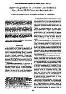
head prior to the echo of the next real discontinuity. In so doing, the first echo present in the de-embedded TDR trace is the echo of the next real discontinuity. III. GENERATING CLUSTERS IN THE SPACE OF POSSIBLE LOOP DISCONTINUITIES Every kind of discontinuity generates a distinct echo whose shape is a function of the discontinuity and the previous loop sections. This can be seen looking at Figure 1, where the echoes generated by four different discontinuities located at a distance of 9 kft from the CO are compared. 1) End of Loop: unterminated loop of 9 kft, AWG 24; 2) Gauge Change (positive): 9 kft of AWG 24, followed by a 6 kft of AWG 26; 3) Gauge Change (negative): 9 kft of AWG 24, followed by a 6 kft of AWG 22; 4) Bridged Tap: 9 kft of AWG 24, followed by a bridged tap of AWG 24 and 2 kft long, followed by another section of 6 kft of AWG 24. As the figure clearly shows, different discontinuities give rise to echoes of considerably different shape. 120
Unterminated
100
80
Amplitude (millivolts)
co-located bridged taps) several tens of topologies may be possible, and the search has to be repeated at every detected discontinuity, thus slowing down identification speed. This paper extends and further improves the techniques presented in [1]-[2] by introducing two novel techniques that reduce computation time [3]. Firstly, we report a method that reduces the number of hypothesized topologies by exploiting a characteristic reported here for the first time: similar discontinuities exhibit similar features so that the set of possible discontinuities can be organized in clusters. Secondly, statistical data is used to improve overall LID accuracy by accounting for the different likelihood of different cable gauges at different distances from a CO.
60 Gauge Change (positive) 40
20
0
-20 Gauge Change (negative) Bridged Tap -40
0
50
100
150
200
250
300
Time (microseconds)
Figure 1: Simulated echo traces representing the shape of the echoes generated by four different discontinuities located at a distance of 9 kft from the CO. Probing signal: 5 V and 5 µs square pulse.
We have also ascertained that similar discontinuities exhibit similar features. For example, let us consider the ranking of the slopes of the TDR trace pertaining to different discontinuities following a 3 kft loop of 26 AWG as shown in Figure 2. We note that the types of discontinuities tend to group in three separate clusters. It also shows that we are very unlikely to mistake a gauge change for a bridged tap, and a little bit less likely to mistake a single bridged tap for two collocated bridged taps. It is therefore useful to organize the set of possible topologies in “families” or clusters, and choose a sample discontinuity per cluster that represents the whole all the echoes caused by successive reflections. The necessity of separating echoes in these two categories is irrelevant for modeling issues, but it becomes important when loop identification is attempted. In fact, any identification algorithm must be able to discriminate between real echoes (the echoes that indicate the actual presence of a real discontinuity) and spurious echoes (the re-reflected and artificial echoes that do not indicate the presence of an additional actual discontinuity).
2
S. Galli, K. Kerpez, “Improved Algorithms for Single Ended Loop Make-Up Identification,” IEEE ICC’06.
family of discontinuities. Preliminary testing is now made on the sample topologies only, and the sample topology that produces the waveform that best matches the observations will define the family of topologies that most likely contains the true topology. The algorithm then limits the search for the best topology within that family of topologies only.
companies nationwide. A survey conducted by Bellcore in 1987-1990 sampled 559 loops at 101 wire centers across the USA. About 24% of the 1983 loop-survey loops were loaded, and about 28% of the Bellcore survey loops were loaded. While these loop surveys are dated, copper cable lengths and gauge as a function of length have not changed much.
0.0000 0
5
10
15
20
25
30
Probability Histogram
-0.0200 26
-0.0400
Gauge Changes
-0.0600 19
Slope
-0.0800 -0.1000
0.12 0.1 0.08 0.06 0.04 0.02
Bridged taps
-0.1200
0
26-26
1 3 5 7 9 11 13 15 17 19 21 23 25 27 29 31 33 35 37 39
Collocated Bridged taps
-0.1400 -0.1600
0.14
35
Loop Working Length (kft) Figure 3: The probability histogram of working lengths measured in the 1983 loop survey.
24-26
19-19
-0.1800
26-26-26
19-22-26
19-19-19
-0.2000
Possible configurations of discontinuities Figure 2: Ranking of the slope (mV/µs) of the TDR trace of three possible discontinuities following a 3 kft loop of AWG 26. Slope is measured in the 911 µs interval; discontinuities consist of one section (gauge change), two sections (bridged taps), and three sections (co-located bridged taps) of infinite length.
IV. ENHANCING LOOP IDENTIFICATION WITH LOOP STATISTICS If some a priori knowledge on the statistical distribution of the loop sections were known, the search could be performed more accurately and efficiently. For example, the algorithm could hypothesize the most recurrent topologies first so that the time needed for the determination of the gauge or for the determination of the kind of discontinuity can be reduced. A partial statistical characterization of the loop plant could be obtained by analyzing the loop records of the CO under test contained in the loop database. A brief overview of statistics of the length and gauge of telephone loops in North America are presented in this section. These statistics provide general information about the loop plant that can be used to enhance loop make up estimation. For example, it is shown that there is very little 19 gauge cable within measurement range of a CO, and that it is uncommon for a loop to have total bridged tap length above 5 kft. Equations for incorporating loop statistics in LID are also presented. IV.A Loop Surveys Statistics from two North American loop surveys are presented here: the 1983 loop survey [6], and an internal Bellcore 1987-1990 loop survey. The 1983 loop survey had a sample of 2290 working loops at 17 different operating
IV.A.1 Working Length Statistics of loop working lengths have been collected on the basis of [6] and Bellcore’s 1987-1990 survey, and are compared here (lengths are in feet): 1983 Survey (Mean: 10,787; Max: 114,103) 90%: --; 75%: 14,100; 50%: 8,890; 25%: 4,440 1987-1990 Bellcore Survey (Mean: 13,092; Max: 90,000) 90%: 25,018; 75%: 18,330; 50%: 11,538; 25%: 5,799 The percentage value expresses the percentage of loops that have working length (feet) less than or equal to the table entry, e.g. the 50% value is the median. The mean, or average, loop working lengths in the Bellcore survey are generally a little longer than those in the 1983 loop survey. The 1983 loop survey gives frequency counts of loop working lengths in 2,000 ft increments. The relative probability histogram of loop working lengths is shown in Figure 3. The 1983 loop survey separated statistics for business and residential loops. The mean working length of business loops was 8,816 ft, and the mean working length of residential loops was 11,723 ft. IV.A.2 Bridged tap length About 27% of the 1983 loop survey loops had no bridged tap. In contrast, 62.6% of the Bellcore survey loops had no bridged tap. Statistics of the total sum of all lengths of bridged taps on a loop with bridged tap are presented here (lengths are in feet): 1983 Survey (Mean: 1,299) Max: 18,374; 90%: --; 75%: 1,760; 50%: 760; 25%: 150 1987-1990 Bellcore Survey (Mean: 1,250) Max: 11,500; 90%: 3,100; 75%: 1,769; 50%: 728; 25%: 317 The percentage value expresses the percentage of loops that have total bridged tap length (feet) less than or equal to the table entry. The probability histogram of total bridged tap
3
S. Galli, K. Kerpez, “Improved Algorithms for Single Ended Loop Make-Up Identification,” IEEE ICC’06.
lengths measured in the 1983 loop survey is shown in Figure 4.
Probability Histogram
0.12 0.1 0.08 0.06 0.04 0.02 0 0.1
0.5
0.9
1.3
1.7
2.1
2.5
2.9
3.3
3.7
4.1
4.5
4.9
5.3
Total Bridged Tap Length (kft) Figure 4: The probability histogram of total bridged tap lengths, measured in the 1983 loop survey (excluding zero lengths).
IV.A.3 Cable gauge In North America, telephone cables are either 26, 24, 22 or 19 American Wire Gauge (AWG). 26 gauge is the thinnest and 19 gauge is the thickest. 26 gauge is prevalent near the CO because it is sufficient for short distances and it uses less duct space. The thicker 24 and 22 gauge become more prevalent at increasing distances from the CO. Distance % AWG26
(kft)
% AWG24
% AWG22
1983 1987-90 1983 1987-90 1983 1987-90
% AWG19 1983
0
72
67
22
25
6
8
0
5
53
53
35
34
12
13
0
10
30
27
51
52
18
21
1
15
16
4
46
62
36
34
2
20
2
2
34
38
60
60
4
26
-
2
-
7
-
90
-
30
0
-
10
-
69
-
21
Overall
40.4
37.8
35.6
40.4
21.3
21.7
2.7
Table 1: Cable gauge statistics from the 1983 and the 1987-90 Bellcore loop surveys. In the 1987-90 Bellcore loop surveys, only 0.1% of cabling overall was 19 gauge, so 19 gauge is omitted from the table.
Cable gauge as a function of distance from the CO is presented in Table 1 for both the 1983 loop survey and the 1987-90 Bellcore survey data. The table also presents overall percentages including all segments of all surveyed loops. The 1987-1990 Bellcore loop survey also contained a large number of measured loop losses on CSA-compatible loops. These were presented as scatter plots of loop length versus loss at 40 kHz, 100 kHz, 200 kHz, and 300 kHz; and were plotted compared to the loss of pure 19, 22, 24, and 26 gauge. A few loops had about the same loss as pure 22 gauge. Many loops had worse loss than pure 26 gauge, particularly at high frequencies. This may be due to bridged taps. The average loop loss appeared to be approximately that of pure 26 gauge.
IV.B Incorporating identification
cable
gauge
statistics
in
loop
Loop statistics can be used to enhance the accuracy of LID over a large population of loops at a wire center. For example, 19 or 22 gauge cable is unlikely close to a CO, and 26 gauge cable is unlikely far from the CO, so these should be weighted as being less probable. To make the estimation of the types of discontinuities more accurate, the loop make-up estimation procedure [2] is extended here to incorporate the prior probabilities of statistics of cable gauge as a function of distance from the CO [3]. Prior probabilities of cable gauges are given in Table 1 for North America. These cable gauge statistics could also be determined separately for a specific wire center or area. The time-sampled vector pulse response of the correct loop model is r, the "noise" or measurement error vector is n, and the actual measured pulse response vector is d = r + n. The measurement error is assumed to be white Gaussian noise, so the ML estimator [2] minimizes the squared error. Loop gauge probabilities are now incorporated with a maximum aposteriori probability (MAP) estimator. Let rˆ be a possible estimate of the gauge of the next section. The prior probabilities pR (rˆ) of each gauge are determined by assuming that the working length is the sum length of all previously estimated loop sections. The MAP estimator selects rˆ to maximize the a-posteriori probability f D| R (d | rˆ) pR (rˆ ) PR| D (rˆ | d ) = (1) f D (d ) where f(⋅) is the probability density function. The denominator is not a function of rˆ so only f D | R (d | rˆ) p R (rˆ ) needs to be maximized. The noise n = d - r is Gaussian so ⎛ 1 1 2⎞ (2) f D | R (d | rˆ) = exp⎜⎜ − d − rˆ ⎟⎟ 2 M 2 M (2π ) σ ⎠ ⎝ 2σ where M is length of the vectors, σ is the standard deviation of the "noise" or measurement error, and
d − rˆ
2
= ∑ iM=1 d i − rˆi
2
is the sum squared error (SSE). The
MAP estimator maximizes f D | R (d | rˆ) p R (rˆ ) , which is the same as maximizing its natural logarithm, ln f D | R (d | rˆ) p R (rˆ ) , and is equivalent to minimizing
(
)
d − rˆ
2
− 2σ 2 ln ( p R (rˆ ))
(3)
Unlike ML estimation, MAP estimation requires knowledge of the standard deviation, σ , of the measurement error. The standard deviation was calculated using measurements on 45 loops with known make-ups. The MAP estimator essentially increases the SSE by the weighting − 2σ 2 ln( p R (rˆ )) , which is large for unlikely gauges with
small pR (rˆ) . The MAP formulas could also be applied to statistics other than cable gauges, such as the probabilities of bridged taps versus working sections.
4
S. Galli, K. Kerpez, “Improved Algorithms for Single Ended Loop Make-Up Identification,” IEEE ICC’06.
V. MEASUREMENT RESULTS A database of actual loop records was assembled to represent a statistically accurate sample of the loop make-ups, as if records were actually drawn from a real wire center. The loop record database contains many fields, including the terminal location, the phone number, the loop ID, the status of the loop, the category of service on the loop, the type of pairgain system on the loop (if any), the cable name, pair number, an indicator as to whether this pair is loaded, as well as the length and gauge information of all the segments of the loop. The database contains data on 10,000 loops with complete records. Loop length statistics were drawn from the sample loop database. Loop length distributions generally have long tails with outliers at very long loop lengths, and a concentration of short to medium loop lengths. Loop length statistics can be accurately modeled by a Gamma probability model [7]. The Gamma cumulative distribution function (CDF) is defined as 1 x Pr(loop length ≤ x ) = ∫ 0 x α −1e − x β dx (4) α Γ(α )β where Γ(α ) = ∫ 0 xα −1e − x dx. . Define ∞
the
mean
of
the
Gamma to be µ, and the standard deviation to be σ. Then µ = αβ, σ2 = αβ2 , so α = (µ2)/(σ2), and β = (σ2)/µ . The working length of a loop is the sum of all cable segment lengths from the CO to the customer location, not including non-working bridged taps. For all 10,000 loops in the sample loop record database, the average working length is 5.60 kft, the standard deviation of the working length is 5.79 kft, the minimum working length is 0.0 kft, and the maximum working length is 50.3 kft. The sample loop database loop working lengths were fit to a Gamma model by equating the first and second moments, with α = 0.935 and β = 5.987. This Gamma model CDF of loop working lengths was found to be in very good agreement with the histogram of all 10,000 sample loop working lengths. The cumulative distribution function (CDF) was used to identify working length as a function of the total percent of the loop plant at this wire center. The following working lengths were identified: the working length which 5% of loops are no longer than, which 10% of loops are no longer than, which 15% of loops are no longer than, ..., and which 95% of loops are no longer than. These working lengths are in the first column in Table 2. Then, a loop make-up in the database was found with about the same working length as that in the first column of Table 2, and is in columns 3-5 of Table 2. These loops were picked to have differing topologies while still being typical. The working lengths are not uniformly distributed, there is some clumping particularly at short 100 or 500 ft lengths, so the percent of loop plant below a working length in Table 2 is only the closest possible approximation. There is no bridged tap information in the sample loop database. Bridged taps are typically found on somewhat less than half of all loops, and are typically relatively short. So, a
single bridged tap was added to six of the loops, and two bridged taps were added to two of the loops. The actual loop make-ups that were measured are in Table 2. These loops allow the accuracy of the LID algorithm to be plotted not only as a function of working length, but also as a function of the percentage of loops at the wire center. The actual individual loop make-ups are compared to their estimates in Table 2. A bridged tap on the end of a loop is the same topology as if the bridged tap were considered a working section, so the length of these end bridged taps were added to the working length. Only one of the loop working length estimates is off by over 20% due to gauge and length estimation error. In particular, the algorithm has found the presence of two far bridged taps in the topology corresponding to the 80% percentile of the wire center but there is substantial error in the estimation of the section lengths. VI. CONCLUSIONS This paper extended work on single-ended LID using enhanced TDR techniques [1], pulse response models, and ML algorithms [2]. A new method for clustering loop topologies was shown [3]. Loop statistics were used to enhance the accuracy of LID across a large number of loops. Pertinent statistics of the loop plant are presented that can be directly applied to enhance overall LID accuracy, for example by accounting for the fact that 22 gauge is uncommon near the CO and 26 gauge is uncommon far from the CO. These were incorporated in an extension of the ML algorithm, with MAP estimation using loop statistics as the prior probabilities. Loops in a sample database of loop records were assembled, measured and identified to asses the accuracy of our algorithms. Once the loop make-up is known, its channel response is easily calculated. Then, knowledge of the noise or crosstalk environment allows the precise calculation of the performance of any DSL type. This knowledge can help enhance the bit rates, service levels, and reliability of DSL services, lowering the number of failures, and helping to enable dynamic spectrum management (DSM) [8]-[11]. REFERENCES [1]
[2]
[3]
[4]
[5]
S. Galli and D. L. Waring, "Loop Makeup Identification Via Single Ended Testing: Beyond Mere Loop Qualification," IEEE J. Select. Areas Commun., Vol. 20, No. 5, June 2002. S. Galli, K. Kerpez, “Signal Processing for Single-Ended Loop Make-Up Identification,” IEEE International Workshop on Signal Processing Advances in Wireless Communications (SPAWC’05), New York City, New York, June 5-8, 2005. S. Galli, K. Kerepz, “Single-Ended Loop Make-Up Identification - Part I and Part II,” submitted to the IEEE Transactions on Instrumentation. and Measurements. T. Bostoen, P. Boets, M. Zekri, L. Van Biesen, T. Pollet, and D. Rabijns, "Estimation of the Transfer Function of a Subscriber Loop by Means of a One-Port Scattering Parameter Measurement at the Central Office," IEEE J. Select. Areas Commun., pp. 936- 948, Vol. 20, No. 5, June 2002. T. Vermeiren, T. Bostoen, P. Boets, X. Ochoa Chebab, F. Louage, “Subscriber loop topology classification by means of time-domain reflectometry,” IEEE International Conference on Communications (ICC'03), May 11-15, 2003.
5
S. Galli, K. Kerpez, “Improved Algorithms for Single Ended Loop Make-Up Identification,” IEEE ICC’06. [6]
[7] [8] [9]
Characterization of Subscriber Loops for Voice and ISDN Services (1983 Subscriber Loop Survey Results), Science and Technology Series, ST-TSY-000041, Bellcore, 1987. K. J. Kerpez, “Statistical Variables for Evaluating Compatibility of Remote Deployments,” Standards contr. T1E1.4/2001-132, May 2001. American National Standard for Telecommunications - Spectrum Management for Loop Transmission Systems, T1.417-2001, Jan. 2001. K. Kerpez, D. Waring, S. Galli J. Dixon, P. Madon, “Advanced DSL Management”, IEEE Communications Magazine, vol. 31, no. 9, September 2003.
[10] K. B. Song, S. T. Chung, G. Ginis, and J. M. Cioffi, "Dynamic Spectrum Management for Next-Generation DSL Systems," IEEE Commun. Magazine, Vol. 40, No. 10, Oct. 2002. [11] K. Kerpez, S. Galli, “Optimization of Single-Carrier and Multi-Carrier DSL Spectra,” IEEE International Conference on Communications, ICC’05, Seoul, Korea, May 16-20, 2005.
Actual loop make-up Approximate % of 1=working, Gauge Feet Working length, ft the wire center 2=bridged tap 538 5 1 26 538
Estimated loop make-up 1=working, Gauge Feet 2=bridged tap 1 26 547
640
10
1
24
640
1
24
634
666
15
1 1
24 26
128 538
1
26
667
896
20
1 2
24 24
640 256
1 2
24 24
636 252
1076
25
1
26
1076
1
26
1074
1280
30
1 2
24 24
896 384
1 2
24 24
886 377
1716
35
1 2
24 24
1076 640
1 2
26 24
622 1080
2074
40
1 1
24 26
1536 538
1
26
1105
4121
45
1 1
26 24
1076 3045
1
24
4219
4896
50
1 1 1
22 24 22
1561 256 3079
1
22
4885
5246
55
1 2
26 24
4606 640
1 2
26 26
4557 640
6309
60
1 2 1 2
26 24 24 24
4133 1536 1536 640
1 2 1 2
26 22 24 24
4201 1431 1511 640
7650
65
1 1
24 26
1536 6114
1 1 1
24 22 26
5443 830 2381
7790
70
1 1 1 1 1
24 22 26 24 22
128 1000 538 3045 3079
1 1
26 24
5588 650
8702
75
1 2
24 26
7626 1076
1 2
24 26
7563 1076
10707
80
1 2 1 2
26 26 26 24
3057 1541 6114 1536
1 2 1 2
26 24 24 22
3262 2135 3518 4950
10756
85
1 1
26 22
4598 6158
1 1
26 22
5185 5345
12192
90
1 1
26 22
3057 9135
1 1
26 24
3130 9157
15305
95
1 2 1
26 26 24
13769 538 1536
1
26
15564
Table 2: Actual loop make-ups, and loop make-ups automatically identified from the single-ended measurements and with no a priori information.
6