Hindawi Publishing Corporation Mathematical Problems in Engineering Volume 2014, Article ID 343514, 8 pages http://dx.doi.org/10.1155/2014/343514
Research Article Improvement of Fuzzy Image Contrast Enhancement Using Simulated Ergodic Fuzzy Markov Chains Behrouz Fathi-Vajargah and Maryam Gharehdaghi Department of Statistics, Faculty of Mathematical Sciences, University of Guilan, P.O. Box 1914, Rasht, Iran Correspondence should be addressed to Behrouz Fathi-Vajargah;
[email protected] Received 30 November 2013; Revised 4 May 2014; Accepted 29 May 2014; Published 26 June 2014 Academic Editor: Rosana Rodriguez-Lopez Copyright © 2014 B. Fathi-Vajargah and M. Gharehdaghi. This is an open access article distributed under the Creative Commons Attribution License, which permits unrestricted use, distribution, and reproduction in any medium, provided the original work is properly cited. This paper presents a novel fuzzy enhancement technique using simulated ergodic fuzzy Markov chains for low contrast brain magnetic resonance imaging (MRI). The fuzzy image contrast enhancement is proposed by weighted fuzzy expected value. The membership values are then modified to enhance the image using ergodic fuzzy Markov chains. The qualitative performance of the proposed method is compared to another method in which ergodic fuzzy Markov chains are not considered. The proposed method produces better quality image.
1. Introduction Fuzzy set theory is useful in managing various uncertainties in computer vision and image processing applications. Fuzzy image processing is a collection of different fuzzy methods to image processing that can comprehend, characterize, and process the images. It has two main phases, namely, image fuzzification and modification of membership values. Image enhancement for brightness transformation valid in many practical cases can be position brightness correction and gray-scale transformation. Position brightness correction adjusts the pixel brightness by taking into account the pixel position in the image. Gray-scale transformation changes the pixel brightness, but it does not take into account the position of the pixels in the image. Gray-scale transformation is just a transformation of the gray scale to another scale to increase the contrast. The purpose of the transformation is to improve the visual appearance of an image. There are many research works on image enhancement [1, 2], but in this paper we focus on ergodic fuzzy Markov chains for image enhancement. Avrachenkov and Sanchez [3] introduced fuzzy Markov chains with a transition possibility measure and a general state space. Also, Kalenatic et al. [4] presented a simulation study on fuzzy Markov chains to identify some characteristics about their behavior, based on matrix analysis. All
the aforementioned investigations show that fuzzy Markov chains have a periodic behavior. We improved behavior of fuzzy Markov chains using Halton sequences and simulated ergodic fuzzy Markov chains [5]. In this paper, we apply our technique of simulating ergodic fuzzy Markov chains for generating membership values of pixels. Enhancement using ergodic fuzzy Markov chains will improve the quality of the image and provide a clear image to the human observer. The overall approach of the paper follows. We consider a low quality fuzzy image with 𝑀 × 𝑁 pixels (𝑥𝑖𝑗 ; 𝑖 = 0, 1 ⋅ ⋅ ⋅ 𝑀 − 1, 𝑗 = 0, 1 ⋅ ⋅ ⋅ 𝑁 − 1). We then obtain the value of threshold 𝑇 of the fuzzy image. The main and novel idea to enhance the image contrast is to consider a pixel as a new image and subdivide it to 𝑛 × 𝑛 pixels. To simulate these 𝑛 × 𝑛 pixels we employ the ergodic fuzzy Markov chains and their transition matrix. For a particular pixel, its related 𝑛 × 𝑛 matrix entries represent membership values of gray levels of the pixel. To increase the image contrast of each pixel using subdivided pixel we use the weighted fuzzy expected value approach based on transition matrix entries of ergodic fuzzy Markov chain. We show that proposed method produces better quality images compared to the fuzzy expected value method given in [1]. In Section 2, we discuss the fuzzy image contrast enhancement. In Section 3, we define the similarity measure
2
Mathematical Problems in Engineering
2500
2000 1500 1000 500 0 0
50
100
150
200
250
Gray levels
Figure 1: Brain MRI and its histogram of gray levels.
and distance measure, and then in Section 4 we review ergodic fuzzy Markov chains. The main result of this paper is presented in Section 5 followed by a simulation study in Section 6. Section 7 shows the performance of our new results based on fuzzy image contrast enhancement using simulated ergodic fuzzy Markov chains. Comparison of our result with original MR image is also presented.
Equation (1) interprets the characteristics of an image with 𝑀 × 𝑁 pixels. The double summations in (1) just refer to a collection of pixels and their membership values not a crisp mathematical summation.
2. Image as a Fuzzy Set, Threshold Technique, and Fuzzy Image Contrast Enhancement
𝑇 = 𝑇 (𝑖, 𝑗, 𝜇 (𝑖, 𝑗) , 𝑓 (𝑖, 𝑗)) ,
The application of fuzzy set theory in image processing took formal shape only in the 1980s with the pioneering research carried out by Pal et al. [6] and Pal and Rosenfeld [2]. 2.1. Image as a Fuzzy Set. The pixel values, which establish an image, may not be accurate and there is basically an intrinsic imprecision or uncertainty embedded in a digital image. While trying to design automated systems for scene analysis and explanation, it may be a good idea to consider the fact that a computer vision system is usually embedded with uncertainty and vagueness, which needs to be taken care of suitably. Proper modeling of this imprecision appearing in a physical phenomenon is an important mission in many applications of image processing. Let 𝐴 be an image of size 𝑀 × 𝑁 having 𝐿 levels and 𝑥𝑖𝑗 the gray level at the pixel position value of the pixels of the image 𝐴 with 0 ≤ 𝜇𝐴 (𝑥𝑖𝑗 ) ≤ 1, where 𝜇𝐴 (𝑥𝑖𝑗 ) = 1 denotes full membership and 𝜇𝐴 (𝑥𝑖𝑗 ) = 0 denotes nonmembership. Intermediate degrees are graded accordingly. Membership values represent the information, say, for example, the brightness, of the pixel at position (𝑖, 𝑗). In fuzzy set theory, an image can be represented as [7] 𝑀−1𝑁−1
∑ ∑ [𝑥𝑖𝑗 , 𝜇𝐴 (𝑥𝑖𝑗 )] , 𝑖=0 𝑗=0
∀𝑥𝑖𝑗 ∈ 𝐴,
𝑖 = 0, 1, 2, . . . , 𝑀 − 1, 𝑗 = 0, 1, 2, . . . , 𝑁 − 1.
(1)
2.2. Fuzzy Threshold Technique. Thresholding is an operation that involves tests against a function 𝑇 of the form (2)
where𝑓(𝑖, 𝑗) is the gray level of pixel (𝑖, 𝑗) and 𝜇(𝑖, 𝑗) denotes some local property of this point. A threshold image 𝑔(𝑖, 𝑗) is defined as 1 𝑔 (𝑖, 𝑗) = { 0
if 𝑓 (𝑖, 𝑗) > 𝑇, if 𝑓 (𝑖, 𝑗) ≤ 𝑇.
(3)
Thus, pixels label 1 (or any other gray level) correspond to objects. However pixels label 0 (or any other gray level not assigned to objects) correspond to the background. When 𝑇 depends only on 𝑓(𝑖, 𝑗) (that is, only on gray level values) the threshold is called global. If 𝑇 depends on both 𝑓(𝑖, 𝑗) and 𝜇(𝑖, 𝑗), the threshold is called local. If, in addition, 𝑇 depends on the spatial coordinates 𝑖 and 𝑗, the threshold is called dynamic or adaptive [7]. Figure 1 captures an MR image, which is not transparent. Its histogram drawn in MATLAB by using pixels properties and their gray levels is also given in this figure. Figures 2 and 3 demonstrate tumor and abdomen images and their related histograms, respectively. As shown in the histograms, in all the cases the ratio of bright pixels to dark ones is low [8, 9]. 2.3. Fuzzy Image Contrast Enhancement. Fuzzy image contrast enhancement is established on gray level mapping from a gray plane into a fuzzy plane using a membership value. It uses the principle of contrast stretching where the image gray levels are transformed in such a way that dark pixels appear much darker and bright pixels appear much brighter. The principle of contrast stretching depends on the selection
Mathematical Problems in Engineering
3 1000
900 800 700 600 500 400 300 200 100 0 0
50
100
150
200
250
Gray levels
Figure 2: Tumor image and its histogram of gray levels.
10000
9000 8000 7000 6000 5000 4000 3000 2000 1000 0 0
50
100
150
200
250
Gray levels
Figure 3: Abdomen image and its histogram of gray levels.
of threshold, 𝑇, so that the gray levels below the threshold 𝑇 are reduced and the gray levels above the threshold 𝑇 are increased in a nonlinear manner. This stretching operation induces saturation at both ends (gray levels): (1 − 𝑏) 𝑥 { { CONT (𝑥) = {𝑥 { {(1 + 𝑎) 𝑥
𝑥 > 𝑡, 𝑥 = 𝑡, 𝑥 < 𝑡.
(4)
CONT(𝑥) is an intensifier stretching that transforms a gray level 𝑥 to an intensified level. 𝑎, 𝑏 are the levels between 0 and 1 that decide the percentage stretching of gray level 𝑥 for a certain threshold “𝑡.” Fuzzy methods for contrast enhancement employ membership values 𝜇(𝑥) to know the degree of brightness or darkness of the pixels in an image. So, ergodic fuzzy Markov chains are used to find the membership values of the pixels in an image that lies in the interval [0, 1] using any membership value. Then, elements of transition possibility matrix of ergodic fuzzy Markov chains are applied on the membership
values to generate new membership values of the pixels in the image [1].
3. Fuzzy Similarity and Distance Measure In this section, fuzzy distance measure is described using fuzzy set theory. Fuzzy distance measure is studied by many authors [10, 11]. We consider a universal set 𝑋 and 𝐹(𝑋) to be a fuzzy set. Let 𝑃(𝑋) be the class of all crisp sets of 𝑋. Also, consider two fuzzy sets, 𝐴 and 𝐵, such that 𝐴, 𝐵 ∈ 𝐹(𝑋). The properties of distance measure between two fuzzy sets 𝐴 and 𝐵 with membership values 𝜇𝐴 (𝑥) and 𝜇𝐵 (𝑥) are given as follows [10]. 3.1. Distance Measure. A function 𝐷 : 𝐹(𝑋)2 → [0, ∞] is called a distance measure if it satisfies the following properties. (1) One has 𝐷(𝐴, 𝐵) = 𝐷(𝐵, 𝐴), ∀𝐴, 𝐵 ∈ 𝐹(𝑋).
4
Mathematical Problems in Engineering (2) For three fuzzy sets 𝐴, 𝐵, 𝐶 ∀𝐴, 𝐵, 𝐶 ∈ 𝐹(𝑋), if 𝐴 ⊂ 𝐵 ⊂ 𝐶 then 𝐷 (𝐴, 𝐵) ≤ 𝐷 (𝐴, 𝐶) and 𝐷(𝐵, 𝐶) ≤ 𝐷(𝐴, 𝐶). (3) One has 𝐷(𝐴, 𝐴) = 0, ∀𝐴 ∈ 𝐹(𝑋). (4) One has 𝐷(𝐶, 𝐶) = max𝐴,𝐵∈𝐹(𝑋) 𝐷(𝐴, 𝐵), ∀𝐶 ∈ 𝑃(𝑋).
For example, consider two fuzzy sets 𝐴 and 𝐵 in a finite 𝑋 = {𝑥1 , 𝑥2 , . . . , 𝑥𝑛 } with 𝜇𝐴 (𝑥) and 𝜇𝐵 (𝑥) as the membership value of sets 𝐴 and 𝐵, respectively. The distance measures are as follow. Hamming Distance. The Hamming distance between two fuzzy sets 𝐴 and 𝐵 is given as 𝑛
𝑑 (𝐴, 𝐵) = ∑ 𝜇𝐴 (𝑥𝑖 ) − 𝜇𝐵 (𝑥𝑖 ) .
(5)
𝑖=1
Euclidean Distance. The Euclidean distance between two fuzzy sets 𝐴 and 𝐵 is given as 𝑛
Definition 1. Let the powers of the fuzzy transition matrix 𝑃 converge in 𝜏 steps to a nonperiodic solution; then the associated fuzzy Markov chain is called aperiodic fuzzy Markov chain and 𝑃∗ = 𝑃𝜏 is its stationary fuzzy transition matrix. Definition 2. A fuzzy Markov chain is called strong ergodic if it is aperiodic and its stationary transition matrix has identical rows. A fuzzy Markov chain is called weakly ergodic if it is aperiodic and its stationary transition matrix is stable with no identical rows. We simulated ergodic fuzzy Markov chains using Halton sequences [5] and make use of them to simulate fuzzy image enhancement. Elements of transition possibility matrix of ergodic fuzzy Markov chains are applied on the membership values to generate new membership values of the pixels in the image. For example 𝜇45 = 0.5 in transition possibility matrix of ergodic fuzzy Markov chains corresponding to image means that the membership value of gray pixel (4, 5) is 0.6.
(6)
Note. Every pixel 𝑥𝑖𝑗 in (1) is considered again as an image with 𝑛 × 𝑛 pixels and is simulated by using transition matrix of ergodic fuzzy Markov chains. For examples the matrix of a pixel is shown as follows.
Let 𝑆 = {1, 2, . . . , 𝑛}. A finite fuzzy set on 𝑆 is defined by a mapping 𝑥 from 𝑆 to [0, 1] represented by a vector 𝑥 = {𝑥1 , 𝑥2 , . . . , 𝑥𝑛 }, with 0 ≤ 𝑥𝑖 ≤ 1, 𝑖 ∈ 𝑆. Here, 𝑥𝑖 is the membership function that a state 𝑖 has regarding a fuzzy set 𝑆, 𝑖 ∈ 𝑆. A fuzzy transition possibility matrix 𝑃 is defined in a metric space 𝑆 × 𝑆 by a matrix {𝜇𝑖𝑗 }𝑛 with 0 ≤ 𝜇𝑖𝑗 ≤ 1,
In Figure 4 we have 8 × 8 pixels represented by 8 × 8 matrix.
2
𝑑 (𝐴, 𝐵) = √ ∑(𝜇𝐴 (𝑥𝑖 ) − 𝜇𝐵 (𝑥𝑖 )) . 𝑖=1
4. Ergodic Fuzzy Markov Chains
𝑖,𝑗=1
𝑖, 𝑗 ∈ 𝑆. 𝜇𝑖𝑗 is the membership value [5]. We note that it does not need elements of each row of the matrix 𝑃 to sum up to one. This fuzzy matrix 𝑃 allows defining all relations among the 𝑚 states of the fuzzy Markov chain at each time instant 𝑡, as follows [3]. At each instant 𝑡, 𝑡 = 1, 2 ⋅ ⋅ ⋅ 𝑙, the state of system is described by the fuzzy set 𝑥(𝑡) . The transition law of a fuzzy Markov chain is given by the fuzzy relational matrix 𝑃 at instant 𝑡, 𝑡 = 1, 2 ⋅ ⋅ ⋅ 𝑙, as follows: 𝑥𝑗(𝑡+1) = max {min {𝑥𝑗(𝑡) , 𝜇𝑖𝑗 }} , 𝑖∈𝑆
𝑥
(𝑡+1)
=𝑥
(𝑡)
𝑗 ∈ 𝑆, (7)
∘ 𝑃,
where 𝑖 and 𝑗, 𝑖, 𝑗 = 1, 2, . . . , 𝑛, are the initial and final states of the transition and 𝑥(0) is the initial distribution. Also, 𝑡−1 𝜇𝑖𝑗𝑡 = max {min {𝜇𝑖𝑘 , 𝜇𝑘𝑗 }} , 𝑘∈𝑆
𝑃𝑡 = 𝑃 ∘ 𝑃𝑡−1 .
𝑖, 𝑗 ∈ 𝑆, (8)
Thomason in [12] shows that the powers of a fuzzy matrix are stable over the max-min operator. More information about powers of a fuzzy matrix can be found in [13]. Now, a stationary distribution of a fuzzy matrix is defined as follows.
5. Fuzzy Image Contrast Enhancement Using Ergodic Fuzzy Markov Chains In recent years, many researchers have applied various fuzzy methods for contrast enhancement [1]. In this paper, we discuss fuzzy expected value method. Fuzzy expected value replaces the mean and median value when treating fuzzy sets. Instead of calculating the average value of a set of numbers, we evaluated a more representative value of a set. This value would indicate a typical grade of membership of a fuzzy set. Consider a fuzzy set 𝐴 in a finite set 𝑋 = {𝑥1 , 𝑥2 . . . , 𝑥𝑛 } with a membership value 𝜇𝐴 : [0, 1]. Let 𝜉𝑇 = {𝑥 | 𝜇𝐴 (𝑥) ≥ 𝑇}, 0 ≤ 𝑇 ≤ 1, represent a subset whose elements are above or equal to the value of the threshold 𝑇 [7]. Then the fuzzy measure defined on the fuzzy subset is 𝜓 (𝜉𝑇 ) =
{number of elements 𝑥 : 𝜇𝐴 (𝑥) ≥ 𝑇} , 𝑁
(9)
where 𝑁 is the number of elements in a set. The fuzzy expected value of 𝜇𝐴 (𝑥) over the fuzzy set is fuzzy expected value = FEV = sup {min {𝑇, 𝜓 (𝜉𝑇 )}} . 0≤𝑇≤1
(10) But FEV does not generate a typical value in some cases. We suggested weighted fuzzy expected value [14] using
Mathematical Problems in Engineering
5
0 0.071 0.142 0.214 0.285 0.357 0.428 0.500
0.071 0.142 0.214 0.285 0.357 0.428 0.500 0.571
0.142 0.214 0.285 0.357 0.428 0.500 0.571 0.642
0.214 0.285 0.357 0.428 0.500 0.571 0.642 0.714
0.285 0.357 0.428 0.500 0.571 0.642 0.714 0.785
0.357 0.428 0.500 0.571 0.642 0.714 0.785 0.857
0.428 0.500 0.571 0.642 0.714 0.785 0.857 0.928
0.500 0.571 0.642 0.714 0.785 0.857 0.928 1
Figure 4
Table 1 𝜇 𝜇𝑖 𝜇𝑗
Pixel number 𝑖 𝑗
𝑚 𝑚𝑖 𝑚𝑗
ergodic fuzzy Markov chains, which gives most typical value of the membership value 𝜇, where weights are applied. The weight is calculated as follows. Consider the two pixels in Table 1, where 𝜇𝑘 is the membership value of the 𝑘th gray level and 𝑚𝑘 is the frequency of occurrence of 𝑘th gray level. (𝑥1 ,𝑥2 ,...,𝑥𝑛 ) Suppose a variational sampling ( (𝑚 ) is given, 1 ,𝑚2 ,...,𝑚𝑛 ) 𝜇𝑖 = 𝜇𝐴 (𝑥𝑖 ), 𝑖 = 1, 2, . . . , 𝑛 are the membership values of some fuzzy set 𝐴 ⊂ 𝑋, 𝜔(𝑥) is a nonnegative monotonically decreasing function defined over the interval [0, 1], and 𝜆 > 1 is a real number. Consider the following equation with respect to 𝑠: 𝑠 = (𝜇1 𝜔 (𝜇1 − 𝑠) 𝑚1𝜆 + 𝜇2 𝜔 (𝜇2 − 𝑠) 𝑚2𝜆 + ⋅ ⋅ ⋅ + 𝜇𝑛 𝜔 (𝜇𝑛 − 𝑠) 𝑚𝑛𝜆 ) × (𝜔 (𝜇1 − 𝑠) 𝑚1𝜆 + 𝜔 (𝜇2 − 𝑠) 𝑚2𝜆
(11)
−1 + ⋅ ⋅ ⋅ + 𝜔 (𝜇𝑛 − 𝑠) 𝑚𝑛𝜆 ) .
𝑠=
𝐷𝑖 = √(𝜓)2 − (𝑔𝑖 )2 .
(13)
The new gray level 𝑔𝑖 is computed as 𝑔𝑖 < 𝜓, 𝑖 = 0, 1, 2, . . . , 𝜓 − 1 max (0, 𝜓 − 𝐷𝑖 ) , { { 𝑔𝑖 = {min (𝐿 − 1, 𝜓 + 𝐷𝑖 ) , 𝑔𝑖 > 𝜓, 𝑖 = 𝜓 + 1, . . . , 𝐿 − 1 { otherwise {𝜓 (14) where 𝑔𝑖 are the final contrast enhanced image using WFEV and ergodic fuzzy Markov chains. 5.1. Algorithm. The algorithm of our approach is as follows.
The solution of (11) is called the weighted fuzzy expected value (WFEV) of order 𝜆 with the attached weight function 𝜔 of membership values (𝜇1 , 𝜇2 . . . 𝜇𝑛 ). The parameter 𝜆 measures the dependence of frequencies of population pixels on the WFEV. Now, we apply WFEV and simulated ergodic fuzzy Markov chains corresponding to image. Each element of transition possibility matrix of ergodic fuzzy Markov chains is 𝜇𝑖 . Suppose that the WFEV for 𝜔(|𝜇𝑖 − 𝑠|) = 𝑒−|𝜇𝑖 −𝑠| , 𝜆 = 2, 𝑠0 = FEV is given by the following form: (−|𝜇𝑖 −𝑠|) 𝜆 𝑚𝑖 ∑𝐿−1 𝑖=0 𝜇𝑖 𝑒 , 𝐿−1 (−|𝜇𝑖 −𝑠|) 𝜆 𝑚𝑖 ∑𝑖=0 𝑒
with 𝑥𝑛+1 = 𝐹(𝑥𝑛 )(𝑠𝑛+1 = 𝐹(𝑠𝑛 )), where 𝑥0 = FEV. This WFEV is used for image enhancement, and when applied on the gray level represents the most typical gray level. For 𝜇𝑖 , we use ergodic fuzzy Markov chains, which in the last simulated by Halton sequences in [5] and use their fuzzy transition matrix corresponding to each pixel of the image. We note that elements of fuzzy transition possibility matrix are membership values of gray levels. If 𝜓 is a simulated gray level corresponding to the WFEV or the FEV and 𝑔𝑖 is the gray level, then the distance measure between 𝜓 and gray level 𝑔𝑖 is given by
(12)
where 𝑖 = 0, 1, 2, . . . , 𝐿 − 1 is the gray levels. The equation for “𝑠” is in the form 𝑥 = 𝐹(𝑥) and is solved iteratively starting
(1) Read the original image. (2) Represent image as a fuzzy set using (1). (3) Represent each pixel 𝑥𝑖𝑗 as a 𝑛 × 𝑛 matrix. (4) Simulate the membership values, that is, matrix entries 𝜇𝑖 , by using ergodic fuzzy Markov chains implemented in [5]. (5) Obtain the value of threshold 𝑇 using [15]. (6) Compute FEV; then set 𝑠0 := FEV. = 𝐹(𝑠𝑛 ), in which 𝐹(𝑠𝑛 ) (7) Put 𝑠𝑛+1 𝐿−1 (−|𝜇𝑖 −𝑠𝑛 |) 𝜆 (−|𝜇𝑖 −𝑠𝑛 |) 𝜆 𝜇 𝑒 𝑚 / ∑ 𝑚𝑖 , (WFEV). ∑𝐿−1 𝑖=0 𝑖 𝑖=0 𝑒 𝑖 (8) Obtain 𝜓(𝜉𝑇 ) using (9). (9) Using (13) simulate the new gray level 𝑔𝑖 .
=
6
Mathematical Problems in Engineering 800 700 600 500 400 300 200 100 0 0
50
100 150 Gray levels
200
250
200
250
Figure 5: Contrast enhancement of brain MRI using FEV and its histogram.
700 600 500 400 300 200 100 0 0
50
100 150 Gray levels
Figure 6: Contrast enhancement of brain MRI using WFEV and ergodic fuzzy Markov chains and its histogram.
800 700 600 500 400 300 200 100 0 0
50
100 150 Gray levels
Figure 7: Contrast enhancement of tumor image using FEV and its histogram.
200
250
Mathematical Problems in Engineering
7
600 500 400 300 200 100 0 0
50
150 100 Gray levels
200
250
Figure 8: Contrast enhancement of tumor image using WFEV and ergodic fuzzy Markov chains and its histogram.
9000 8000 7000 6000 5000 4000 3000 2000 1000 0 0
50
100 150 Gray levels
200
250
Figure 9: Contrast enhancement of abdomen image using FEV and its histogram. 8000 7000 6000 5000 4000 3000 2000 1000 0 0
50
100 150 Gray levels
200
250
Figure 10: Contrast enhancement of abdomen image using WFEV and ergodic fuzzy Markov chains and its histogram.
6. Simulation Consider a low contrast image. We apply FEV and WFEV methods to improve the image contrast. These methods are presented in the last section. In our proposed approach, considering each pixel as a new image and simulating membership values of pixel using the transition matrix of
ergodic fuzzy Markov chain and applying WFEV method, we would enhance the image contrast. Figure 5 and its related histogram depict the contrast enhancement of the image using FEV method. Figure 6 also shows the same improvement in image contrast using WFEV and ergodic fuzzy Markov chains. As shown in histograms, the number of dark pixels in Figure 5 is less than those in Figure 2, and
8 the number of dark pixels in Figure 6 is less than those in Figure 5, exhibiting that using ergodic fuzzy Markov chain along with employing WFEV method is a superior approach compared to the others. The same inference results from Figures 7 and 8 as well as Figures 9 and 10. We have employed MATLAB software to implement this approach.
7. Conclusion In this paper, using simulated ergodic fuzzy Markov chains given in [5] and WFEV method we not only enhance the (MRI) low image in Figures 6, 8, and 10 but we also obtain better results than those resulted from FEV approach without considering ergodic fuzzy Markov chains for 𝜇𝑖 . This can be seen from simulation study of Section 6. As we subdivide pixels to smaller pixels and treating each new smaller pixel as an image and employing the simulation phase for the image, we would improve the quality of the original image. We hope to employ ergodic fuzzy Markov chains for contrast improvement using an intensification operator (INT approach).
Conflict of Interests The authors declare that there is no conflict of interests regarding the publication of this paper.
References [1] B. Jayaram, K. V. V. D. L. Narayana, and V. Vetrivel, “Fuzzy inference system based contrast enhancement,” in Proceedings of the 7th Conference of the European Society for Fuzzy Logic and Technology (EUSFLAT '11), pp. 311–318, Aix-les-Bains, France, July 2011. [2] S. K. Pal and A. Rosenfeld, “Image enhancement and thresholding by optimization of fuzzy compactness,” Pattern Recognition Letters, vol. 7, no. 2, pp. 77–86, 1988. [3] K. E. Avrachenkov and E. Sanchez, “Fuzzy Markov chains,” in Proceedings of the 8th Conference on Information Processing and Management of Uncertainty in Knowledge-Based Systems (IPMU '00), pp. 1851–1856, Madrid, Spain, 2000. [4] D. Kalenatic, J. Figueroa-Garcia, and C. A. Lopez, “Scalarization of type-1 fuzzy markov chains,” in Advanced Intelligent Computing Theories and Applications, Lecture Notes in Computer Science, pp. 110–117, Springer, Berlin, Germany, 2010. [5] B. Fathi Vajargaha and M. Gharehdaghi, “Reducing periodicity of fuzzy Markov chains based on simulation using Halton sequence,” Communications in Statistics—Simulation and Computation, 2014. [6] S. K. Pal, R. A. King, and A. Hashim, “Automatic grey level thresholding through index of fuzziness and entropy,” Pattern Recognition Letters, vol. 1, no. 3, pp. 141–146, 1983. [7] T. Chaira and A. K. Ray, “Threshold selection using fuzzy set theory,” Pattern Recognition Letters, vol. 25, no. 8, pp. 865–874, 2004. [8] http://www.radiologyinfo.org/. [9] https://www.dartmouth.edu/∼anatomy/Abdomen/kidney/ radiology/MRIcoronal.htm.
Mathematical Problems in Engineering [10] Z. C. Johaniyak and S. Kovacs, “Distance based similarity measures on fuzzy sets,” in Proceedings of the 3rd Slovakian-Hungarian Joint Symposium on Applied Machine Intelligence (SAMI '05), Herl’ani, Slovakia, January 2005. [11] W. Sander, “On measures of fuzziness,” Fuzzy Sets and Systems, vol. 29, no. 1, pp. 49–55, 1989. [12] M. Thomason, “Convergence of powers of a fuzzy matrix,” Journal of Mathematical Analysis and Applications, vol. 57, no. 2, pp. 476–480, 1977. [13] M. Gavalec, “Periods of special fuzzy matrices,” Tatra Mountains Mathematical Publication, vol. 16, pp. 47–60, 1999. [14] G. Sirbiladze, A. Sikharulidze, and N. Sirbiladze, “Generalized weighted fuzzy expected values in uncertainty environment,” in Proceedings of the 9th WSEAS International Conference on Artificial Intelligence, Knowledge Engineering and Data Bases, pp. 59–64, World Scientific and Engineering Academy and Society, Stevens Point, Wis, USA, 2010. [15] L.-K. Huang and M.-J. J. Wang, “Image thresholding by minimizing the measures of fuzziness,” Pattern Recognition, vol. 28, no. 1, pp. 41–51, 1995.
Advances in
Operations Research Hindawi Publishing Corporation http://www.hindawi.com
Volume 2014
Advances in
Decision Sciences Hindawi Publishing Corporation http://www.hindawi.com
Volume 2014
Journal of
Applied Mathematics
Algebra
Hindawi Publishing Corporation http://www.hindawi.com
Hindawi Publishing Corporation http://www.hindawi.com
Volume 2014
Journal of
Probability and Statistics Volume 2014
The Scientific World Journal Hindawi Publishing Corporation http://www.hindawi.com
Hindawi Publishing Corporation http://www.hindawi.com
Volume 2014
International Journal of
Differential Equations Hindawi Publishing Corporation http://www.hindawi.com
Volume 2014
Volume 2014
Submit your manuscripts at http://www.hindawi.com International Journal of
Advances in
Combinatorics Hindawi Publishing Corporation http://www.hindawi.com
Mathematical Physics Hindawi Publishing Corporation http://www.hindawi.com
Volume 2014
Journal of
Complex Analysis Hindawi Publishing Corporation http://www.hindawi.com
Volume 2014
International Journal of Mathematics and Mathematical Sciences
Mathematical Problems in Engineering
Journal of
Mathematics Hindawi Publishing Corporation http://www.hindawi.com
Volume 2014
Hindawi Publishing Corporation http://www.hindawi.com
Volume 2014
Volume 2014
Hindawi Publishing Corporation http://www.hindawi.com
Volume 2014
Discrete Mathematics
Journal of
Volume 2014
Hindawi Publishing Corporation http://www.hindawi.com
Discrete Dynamics in Nature and Society
Journal of
Function Spaces Hindawi Publishing Corporation http://www.hindawi.com
Abstract and Applied Analysis
Volume 2014
Hindawi Publishing Corporation http://www.hindawi.com
Volume 2014
Hindawi Publishing Corporation http://www.hindawi.com
Volume 2014
International Journal of
Journal of
Stochastic Analysis
Optimization
Hindawi Publishing Corporation http://www.hindawi.com
Hindawi Publishing Corporation http://www.hindawi.com
Volume 2014
Volume 2014