plied in an attempt to use not only the gradient of the error function but also the second ... thermore, it is not certain that the extra computational cost speeds up the minimization process for nonconvex functions when far from a minimizer, .... the learning rate is a weighted average of the direction cosines of weight changes at ...
LETTER
Communicated by Nicol Schraudolph
Improving the Convergence of the Backpropagation Algorithm Using Learning Rate Adaptation Methods G. D. Magoulas Department of Informatics, University of Athens, GR-157.71, Athens, Greece University of Patras Artificial Intelligence Research Center (UPAIRC), University of Patras, GR-261.10 Patras, Greece
M. N. Vrahatis G. S. Androulakis Department of Mathematics, University of Patras, GR-261.10, Patras, Greece University of Patras Artificial Intelligence Research Center (UPAIRC), University of Patras, GR-261.10 Patras, Greece
This article focuses on gradient-based backpropagation algorithms that use either a common adaptive learning rate for all weights or an individual adaptive learning rate for each weight and apply the Goldstein/Armijo line search. The learning-rate adaptation is based on descent techniques and estimates of the local Lipschitz constant that are obtained without additional error function and gradient evaluations. The proposed algorithms improve the backpropagation training in terms of both convergence rate and convergence characteristics, such as stable learning and robustness to oscillations. Simulations are conducted to compare and evaluate the convergence behavior of these gradient-based training algorithms with several popular training methods.
1 Introduction The goal of supervised training is to update the network weights iteratively to minimize globally the difference between the actual output vector of the network and the desired output vector. The rapid computation of such a global minimum is a rather difficult task since, in general, the number of network variables is large and the corresponding nonconvex multimodal objective function possesses multitudes of local minima and has broad flat regions adjoined with narrow steep ones. The backpropagation (BP) algorithm (Rumelhart, Hinton, & Williams, 1986) is widely recognized as a powerful tool for training feedforward neural networks (FNNs). But since it applies the steepest descent (SD) method c 1999 Massachusetts Institute of Technology Neural Computation 11, 1769–1796 (1999) °
1770
G. D. Magoulas, M. N. Vrahatis, and G. S. Androulakis
to update the weights, it suffers from a slow convergence rate and often yields suboptimal solutions (Gori & Tesi, 1992). A variety of approaches adapted from numerical analysis have been applied in an attempt to use not only the gradient of the error function but also the second derivative in constructing efficient supervised training algorithms to accelerate the learning process. However, training algorithms that apply nonlinear conjugate gradient methods, such as the FletcherReeves or the Polak-Ribiere methods (Møller, 1993; Van der Smagt, 1994), or variable metric methods, such as the Broyden-Fletcher-Goldfarb-Shanno method (Watrous, 1987; Battiti, 1992), or even Newton’s method (Parker, 1987; Magoulas, Vrahatis, Grapsa, & Androulakis, 1997), are computationally intensive for FNNs with several hundred weights: derivative calculations as well as subminimization procedures (for the case of nonlinear conjugate gradient methods) and approximations of various matrices (for the case of variable metric and quasi-Newton methods) are required. Furthermore, it is not certain that the extra computational cost speeds up the minimization process for nonconvex functions when far from a minimizer, as is usually the case with the neural network training problem (Dennis & Mor´e, 1977; Nocedal, 1991; Battiti, 1992). Therefore, the development of improved gradient-based BP algorithms is a subject of considerable ongoing research. The research usually focuses on heuristic methods for dynamically adapting the learning rate during training to accelerate the convergence (see Battiti, 1992, for a review on these methods). To this end, large learning rates are usually utilized, leading, in certain cases, to fluctuations. In this article we propose BP algorithms that incorporate learning-rate adaptation methods and apply the Goldstein-Armijo line search. They provide stable learning, robustness to oscillations, and improved convergence rate. The article is organized as follows. In section 2 the BP algorithm is presented, and three new gradient-based BP algorithms are proposed. Experimental results are presented in section 3 to evaluate and compare the performance of these algorithms with several other BP methods. Section 4 presents the conclusions.
2 Gradient-based BP Algorithms with Adaptive Learning Rates To simplify the formulation of the equations throughout the article, we use a unified notation for the weights. Thus, for an FNN with a total of n weights, Rn is the n–dimensional real space of column weight vectors w with components w1 , w2 , . . . , wn , and w∗ is the optimal weight vector with components w∗1 , w∗2 , . . . , w∗n ; E is the batch error measure defined as the sum-of-squared-differences error function over the entire training set; ∂i E(w) denotes the partial derivative of E(w) with respect to the ith variable wi ; g(w) = (g1 (w), . . . , gn (w)) defines the gradient ∇E(w) of the sum-
Improving the Convergence of the Backpropagation Algorithm
1771
of-squared-differences error function E at w, while H = [Hij ] defines the Hessian ∇ 2 E(w) of E at w. In FNN training, the minimization of the error function E using the BP algorithm requires a sequence of weight iterates {wk }∞ k=0 , where k indicates iterations (epochs), which converges to a local minimizer w∗ of E. The batchtype BP algorithm finds the next weight iterate using the relation wk+1 = wk − ηg(wk ),
(2.1)
where wk is the current iterate, η is the constant learning rate, and g(w) is the gradient vector, which is computed by applying the chain rule on the layers of an FNN (see Rumelhart et al., 1986). In practice the learning rate is usually chosen 0 < η < 1 to ensure that successive steps in the weight space do not overshoot the minimum of the error surface. In order to ensure global convergence of the BP algorithm, that is, convergence to a local minimizer of the error function from any starting point, the following assumptions are needed (Dennis & Schnabel, 1983; Kelley, 1995): 1. The error function E is a real–valued function defined and continuous everywhere in Rn , bounded below in Rn . 2. For any two points w and v ∈ Rn , ∇E satisfies the Lipschitz condition, k∇E(w) − ∇E(v)k ≤ Lkw − vk,
(2.2)
where L > 0 denotes the Lipschitz constant. The effect of the above assumptions is to place an upper bound on the degree of the nonlinearity of the error function, via the curvature of E, and to ensure that the first derivatives are continuous at w. If these assumptions are fulfilled, the BP algorithm can be made globally convergent by determining the learning rate in such a way that the error function is exactly subminimized along the direction of the negative of the gradient in each iteration. To this end, an iterative search, which is often expensive in terms of error function evaluations, is required. To alleviate this situation, it is preferable to determine the learning rate so that the error function is sufficiently decreased on each iteration, accompanied by a significant change in the value of w. The following conditions, associated with the names of Armijo, Goldstein, and Price (Ortega & Rheinboldt, 1970), are used to formulate the above ideas and to define a criterion of acceptance of any weight iterate: °2 ° ´ ³ ° ° E wk − ηk g(wk ) − E(wk ) ≤ −σ1 ηk °∇E(wk )° , °2 ° ´> ³ ° ° ∇E wk − ηk g(wk ) g(wk ) ≥ σ2 °∇E(wk )° ,
(2.3) (2.4)
1772
G. D. Magoulas, M. N. Vrahatis, and G. S. Androulakis
where 0 < σ1 < σ2 < 1. Thus, by selecting an appropriate value for the learning rate, we seek to satisfy conditions 2.3 and 2.4. The first condition ensures that using ηk , the error function is reduced at each iteration of the algorithm and the second condition prevents ηk from becoming too small. Moreover, conditions 2.3–2.4 have been shown (Wolfe, 1969, 1971) to be sufficient to ensure global convergence for any algorithm that uses local minimization methods, which is the case of Fletcher-Reeves, Polak-Ribiere, Broyden-Fletcher-Goldfarb-Shanno, or even Newton’s method-based training algorithms, provided the search directions are not orthogonal to the direction of steepest descent at wk . In addition, these conditions can be used in learning-rate adaptation methods to enhance BP training with tuning techniques that are able to handle arbitrary large learning rates. A simple technique to tune the learning rates, so that they satisfy conditions 2.3–2.4 in each iteration, is to decrease ηk by a reduction factor 1/q, where q > 1 (Ortega & Rheinboldt, 1970). This means that ηk is decreased by the largest number in the sequence {q−m }∞ m=1 , so that condition 2.3 is satisfied. The choice of q is not critical for successful learning; however, it has an influence on the number of error function evaluations required to obtain an acceptable weight vector. Thus, some training problems respond well to one or two reductions in the learning-rate by modest amounts (such as 1/2), and others require many such reductions, but might respond well to a more aggressive learning-rate reduction (for example, by factors of 1/10, or even 1/20). On the other hand, reducing ηk too much can be costly since the total number of iterations will be increased. Consequently, when seeking to satisfy condition 2.3, it is important to ensure that the learning rate is not reduced unnecessarily so that condition 2.4 is not satisfied. Since, in the BP algorithms, the gradient vector is known only at the beginning of the iterative search for an acceptable weight vector, condition 2.4 cannot be checked directly (this task requires additional gradient evaluations in each iteration of the training algorithm), but is enforced simply by placing a lower bound on the acceptable values of the ηk . This bound on the learning rate has the same theoretical effect as condition 2.4 and ensures global convergence (Shultz, Schnabel, & Byrd, 1982; Dennis & Schnabel, 1983). Another approach to perform learning-rate reduction is to estimate the appropriate reduction factor in each iteration. This is achieved by modeling the decrease in the magnitude of the gradient vector as the learning rate is reduced. To this end, quadratic and cubic interpolations are suggested that exploit the available information about the error function. Relative techniques have been proposed by Dennis and Schnabel (1983) and Battiti (1989). A different approach to decrease the learning rate gradually is the socalled search–then–converge schedules that combine the desirable features of the standard least-mean-square and traditional stochastic approximation algorithms (Darken, Chiang, & Moody, 1992). Alternatively, several methods have been suggested to adapt the learning rate during training. The adaptation is usually based on the following
Improving the Convergence of the Backpropagation Algorithm
1773
approaches: (1) start with a small learning rate and increase it exponentially if successive iterations reduce the error, or rapidly decrease it if a significant error increase occurs (Vogl, Mangis, Rigler, Zink, & Alkon, 1988; Battiti, 1989), (2) start with a small learning rate and increase it if successive iterations keep gradient direction fairly constant, or rapidly decrease it if the direction of the gradient varies greatly at each iteration (Chan & Fallside, 1987) and (3) for each weight an individual learning rate is given, which increases if the successive changes in the weights are in the same direction and decreases otherwise. The well-known delta-bar-delta method (Jacobs, 1988) and Silva and Almeida’s method (1990) follow this approach. Another method, named quickprop, has been presented in Fahlman (1989). Quickprop is based on independent secant steps in the direction of each weight. Riedmiller and Braun (1993) proposed the Rprop algorithm. The algorithm updates the weights using the learning rate and the sign of the partial derivative of the error function with respect to each weight. This approach accelerates training mainly in the flat regions of the error function (Pfister & Rojas, 1993; Rojas, 1996). Note that all the learning-rate adaptation methods mentioned employ heuristic coefficients in an attempt to secure converge of the BP algorithm to a minimizer of E and to avoid oscillations. A different approach is to exploit the local shape of the error surface as described by the direction cosines or the Lipschitz constant. In the first case, the learning rate is a weighted average of the direction cosines of weight changes at the current and several previous successive iterations (Hsin, Li, Sun, & Sclabassi, 1995), while in the second case ηk is an approximation of the Lipschitz constant (Magoulas, Vrahatis, & Androulakis, 1997). In what follows, we present three globally convergent BP algorithms with adaptive convergence rates. 2.1 BP Training Using Learning Rate Adaptation. Goldstein’s and Armijo’s work on steepest–descent and gradient methods provides the basis for constructing training procedures with adaptive learning rate. The method of Goldstein (1962) requires the assumption that E ∈ C2 (i.e., twice continuously differentiable) on S (w0 ), where S (w0 ) = {w: E(w) ≤ E(w0 )} is bounded, for some initial vector w0 . It also requires that η is chosen to satisfy the relation sup kH(w)k ≤ η−1 < ∞ in some bounded region where the relation E(w) ≤ E(w0 ) holds. The kth iteration of the algorithm consists of the following steps: Step 1. Choose η0 to satisfy sup kH(w)k ≤ η0−1 < ∞ and δ to satisfy 0 < δ ≤ η0 . Step 2. Set ηk = η, where η is such that δ ≤ η ≤ 2η0 − δ and go to the next step. Step 3. Update the weights wk+1 = wk − ηk g(wk ).
1774
G. D. Magoulas, M. N. Vrahatis, and G. S. Androulakis
However, the manipulation of the full Hessian is too expensive in computation and storage for FNNs with several hundred weights (Becker & Le Cun, 1988). Le Cun, Simard, & Pearlmutter (1993) proposed a technique, based on appropriate perturbations of the weights, for estimating on–line the principal eigenvalues and eigenvectors of the Hessian without calculating the full matrix H. According to experiments reported in Le Cun et al. (1993), the largest eigenvalue of the Hessian is mainly determined by the FNN architecture, the initial weights, and short–term, low–order statistics of the training data. This technique could be used to determine η0 , in step 1 of the above algorithm, requiring additional presentations of the training set in the early training. A different approach is based on the work of Armijo (1966). Armijo’s modified SD algorithm automatically adapts the rate of convergence and converges under less restrictive assumptions than those imposed by Goldstein. In order to incorporate Armijo’s search method for the adaptation of the learning rate in the BP algorithm, the following assumptions are needed: 1. The function E is a real–valued function defined and continuous everywhere in Rn , bounded below in Rn . 2. For w0 ∈ Rn define S (w0 ) = {w: E(w) ≤ E(w0 )}, then E ∈ C1 on S (w0 ) and ∇E is Lipschitz continuous on S (w0 ), that is, there exists a Lipschitz constant L > 0, such that k∇E(w) − ∇E(v)k ≤ Lkw − vk,
(2.5)
for every pair w, v ∈ S(w0 ), 3. r > 0 implies that m(r) > 0, where m(r) = infw∈Sr (w0 ) k∇E(w)k, Sr (w0 ) = Sr ∩ S (w0 ), Sr = {w: kw − w∗ k ≥ r}, and w∗ is any point for which E(w∗ ) = infw∈Rn E(w), (if Sr (w0 ) is void, we define m(r) = ∞). If the above assumptions are fulfilled and ηm = η0 /qm−1 , m = 1, 2, . . . , with η0 an arbitrary initial learning rate, then the sequence 2.1 can be written as wk+1 = wk − ηmk g(wk ),
(2.6)
where mk is the smallest positive integer for which °2 ° ´ ³ 1 ° ° E wk − ηmk g(wk ) − E(wk ) ≤ − ηmk °∇E(wk )° , 2
(2.7)
and it converges to the weight vector w∗ , which minimizes the function E (Armijo, 1966; Ortega & Rheinboldt, 1970). Of course, this adaptation method does not guarantee finding the optimal learning rate but only an acceptable one, so that convergence is obtained and oscillations are avoided.
Improving the Convergence of the Backpropagation Algorithm
1775
This is achieved using the inequality 2.7 which ensures that the error function is sufficiently reduced at each iteration. Next, we give a procedure that combines this method with the batch BP algorithm. Note that the vector g(wk ) is evaluated over the entire training set as in the batch BP algorithm, and the value of E at wk is computed with a forward pass of the training set through the FNN. Algorithm-1: BP with Adaptive Learning Rate. Initialization. Randomly initialize the weight vector w0 and set the maximum number of allowed iterations MIT, the initial learning rate η0 , the reduction factor q, and the desired error limit ε. Recursion. For k = 0, 1, . . . , MIT. 1. Set η = η0 , m = 1, and go to the next step. ¢ ¡ 2. If E wk − ηg(wk ) − E(wk ) ≤ − 12 ηk∇E(wk )k2 , go to step 4; otherwise, set m = m + 1 and go to the next step. 3. Set η = η0 /qm−1 , and return to step 2. 4. Set wk+1 = wk − ηg(wk ).
¢ ¡ 5. If the convergence criterion E wk − ηg(wk ) ≤ ε is met, then terminate; otherwise go to the next step. 6. If k < MIT, increase k and begin recursion; otherwise terminate. Termination. Get the final weights wk+1 , the corresponding error value E(wk+1 ), and the number of iterations k. Clearly, algorithm-1 is able to handle arbitrary learning rates, and, in this way, learning by neural networks on a first-time basis for a given problem becomes feasible. 2.2 BP Training by Adapting a Self-Determined Learning Rate. The work of Cauchy (1847) and Booth (1949) suggests determining the learning rate ηk by a Newton step for the equation E(wk − ηdk ) = 0, for the case that E: Rn → R satisfies E(w) ≥ 0 ∀w ∈ Rn . Thus ηk = E(wk )/g(wk )> (dk ), where dk denotes the search direction. When dk = g(wk ), the iterative scheme 2.1 is reformulated as: "
w
k+1
E(wk ) =w − k∇E(wk )k2 k
# g(wk ).
(2.8)
1776
G. D. Magoulas, M. N. Vrahatis, and G. S. Androulakis
The iterations (see equation 2.8) constitute a gradient method that has been studied by Altman (1961). Obviously, the iterative scheme, 2.8, takes into consideration information from both the error function and the gradient magnitude. When the gradient magnitude is small, the local shape of E is flat; otherwise it is steep. The value of the error function indicates how close to the global minimizer this local shape is. Taking into consideration the above pieces of information, the iterative scheme, 2.8, is able to escape from local minima located far from the global minimizer. In general, the error function has broad, flat regions adjoined with narrow steep ones. This causes the iterative scheme, 2.8, to create very large learning rates due to the small values of the denominator, pushing the neurons into saturation, and thus it exhibits pathological convergence behavior. In order to alleviate this situation and eliminate the possibility of using an unsuitable self-determined learning rate, denoted by η0 , we suggest a proper learning rate “tuning.” Therefore, we decide whether the obtained weight vector is acceptable by considering if condition 2.7 is satisfied. Unacceptable vectors are redefined using learning rates defined by the relation ηk = η0 /qmk −1 , for mk = 1, 2, . . . Moreover, this strategy allows using one-dimensional minimization of the error function without losing global convergence. A high-level description of the proposed algorithm that combines BP training with the learning-rate adaptation method follows: Algorithm-2: BP with Adaptation of a Self-Determined Learning Rate. Initialization. Randomly initialize the weight vector w0 and set the maximum number of allowed iterations MIT, the reduction factor q and the desired error limit ε. Recursion. For k = 0, 1, . . . , MIT. 1. Set m = 1, and go to the next step. 2. Set η0 = E(wk )/k∇E(wk )k2 ; also set η = η0 . 3. If E(wk − ηg(wk )) − E(wk ) ≤ − 12 ηk∇E(wk )k2 go to step 5; otherwise, set m = m + 1 and go to the next step. 4. Set η = η0 /qm−1 and return to step 3. 5. Set wk+1 = wk − ηg(wk ).
¢ ¡ 6. If the convergence criterion E wk − ηg(wk ) ≤ ε is met, then terminate; otherwise go to the next step. 7. If k < MIT, increase k and begin recursion; otherwise terminate. Termination. Get the final weights wk+1 , the corresponding error value E(wk+1 ), and the number of iterations k.
Improving the Convergence of the Backpropagation Algorithm
1777
2.3 BP Training by Adapting a Different Learning Rate for Each Weight Direction. Studying the sensitivity of the minimizer to small changes by approximating the error function quadratically, it is known that in a sufficiently small neighborhood of w∗ , the directions of the principal axes of the corresponding elliptical contours (n-dimensional ellipsoids) will be given by the eigenvectors of ∇ 2 E(w∗ ), while the lengths of the axes will be inversely proportional to the square roots of the corresponding eigenvalues. Hence, a variation along the eigenvector corresponding to the maximum eigenvalue will cause the largest change in E, while the eigenvector corresponding to the minimum eigenvalue gives the least sensitive direction. Thus, in general, a learning rate appropriate in one weight direction is not necessarily appropriate for other directions. Moreover, it may not be appropriate for all the portions of a general error surface. Thus, the fundamental algorithmic issue is to find the proper learning rate that compensates for the small magnitude of the gradient in the flat regions and dampens the large weight changes in highly deep regions. A common approach to avoid slow convergence in the flat directions and oscillations in the steep directions, as well as to exploit the parallelism inherent in the evaluation of E(w) and g(w) by the BP algorithm, consists of using a different learning rate for each direction in weight space (Jacobs, 1988; Fahlman, 1989; Silva & Almeida, 1990; Pfister & Rojas, 1993; Riedmiller & Braun, 1993). However, attempts to find a proper learning rate for each weight usually result in a trade-off between the convergence speed and the stability of the training algorithm. For example, the delta-bar-delta method (Jacobs, 1988) or the quickprop method (Fahlman, 1989) introduces additional highly problem-dependent heuristic coefficients to alleviate the stability problem. Below, we derive a new method that exploits the local information regarding the direction and the morphology of the error surface at the current point in the weight space in order to adapt dynamically a different learning rate for each weight. This learning-rate adaptation is based on estimation of the local Lipschitz constant along each weight direction. It is well known that the inverse of the Lipschitz constant L can be used to obtain the optimal learning rate, which is 0.5L−1 (Armijo, 1966). Thus, in the steep regions of the error surface, L is large, and a small value for the learning rate is used in order to guarantee convergence. On the other hand, when the error surface has flat regions, L is small, and a large learning rate is used to accelerate the convergence speed. However, in neural network training, neither the morphology of the error surface nor the value of L is known a priori. Therefore, we take the maximum (infinity) norm in order to obtain a local estimation of the Lipschitz constant L (see relation 2.5) as follows: 3k = max |∂j E(wk ) − ∂j E(wk−1 )|/ max |wjk − wjk−1 |, 1≤j≤n
1≤j≤n
(2.9)
1778
G. D. Magoulas, M. N. Vrahatis, and G. S. Androulakis
where wk and wk−1 are a pair of consecutive weight updates at the kth iteration. In order to take into consideration the shape of the error surface to adapt dynamically a different learning rate for each weight, we estimate 3k along the ith direction, i = 1, . . . , n, at the kth iteration by |, 3ki = |∂i E(wk ) − ∂i E(wk−1 )|/|wki − wk−1 i
(2.10)
and we use the inverse of 3ki to estimate the learning rate of the ith coordinate direction. The reason for choosing 3ki instead of 3k is that when large changes of the ith weight occur and the error surface along the ith direction is flat, we have to take a larger learning rate along this direction. This can be done by taking equation 2.10 instead of 2.9, since in this case equation 2.10 underestimates 3k . On the other hand, when small changes of the ith weight occur and the error surface along the ith direction is steep, equation 2.10 overestimates 3k , and thus the learning rate to this direction is dynamically reduced in order to avoid oscillations. Therefore, the larger the value of 3ki is, the smaller learning rate is used and vice versa. As a consequence, the iterative scheme, equation 2.1, is reformulated as: n o wk+1 = wk − γk diag 1/3k1 , . . . , 1/3kn ∇E(wk ),
(2.11)
where γk is a relaxation coefficient. By properly running γk , we are able to avoid temporary oscillations and/or to enhance the rate of convergence when we are far from a minimum. A search technique for γk consists of finding the weight vectors of the sequence {wk }∞ k=0 that satisfy the following condition: °2 ° o n 1 ° ° E(wk+1 ) − E(wk ) ≤ − γmk °diag 1/3k1 , . . . , 1/3kn ∇E(wk )° . 2
(2.12)
If a weight vector wk+1 does not satisfy the above condition, it has to be evaluated again using Armijo’s search method. In this case, Armijo’s search method gradually reduces inappropriate γk values to acceptable ones by finding the smallest positive integer mk = 1, 2, . . . such that γmk = γ0 /qmk −1 satisfies condition 2.12. The BP algorithm, in combination with the above learning-rate adaptation method, provides an accelerated training procedure. A high-level description of the new algorithm is given below. Algorithm-3: BP with Adaptive Learning Rate for Each Weight. Initialization. Randomly initialize the weight vector w0 and set the maximum number of allowed iterations MIT, the initial relaxation coefficient γ0 ,
Improving the Convergence of the Backpropagation Algorithm
1779
the initial learning rate for each weight η0 , the reduction factor q, and the desired error limit ε. Recursion. For k = 0, 1, . . . , MIT. 1. Set γ = γ0 , m = 1, and go to the next step. |, i = 1, . . . , n; 2. If k ≥ 1 set 3ki = |∂i E(wk ) − ∂i E(wk−1 )|/|wki − wk−1 i otherwise set 3k = η0−1 I. 3. If E(wk − γ diag{1/3k1 , . . . , 1/3kn }∇E(wk )) − E(wk ) ≤ − 12 γ k diag{1/3k1 , . . . , 1/3kn }∇E(wk )k2 , go to step 5; otherwise, set m = m + 1 and go to the next step. 4. Set γ = γ0 /qm−1 , and return to step 3. 5. Set wk+1 = wk − γ diag{1/3k1 , . . . , 1/3kn }∇E(wk ). 6. If the convergence criterion E(wk − γ diag{1/3k1 , . . . , 1/3kn }∇E(wk )) ≤ ε is met then terminate; otherwise go to the next step. 7. If k < MIT, increase k and begin recursion; otherwise terminate. Termination. Get the final weights wk+1 , the corresponding error value E(wk+1 ), and the number of iterations k. A common characteristic of all the methods that adapt a different learning rate for each weight is that they require at each iteration the global information obtained by taking into consideration all the coordinates. To this end, learning-rate lower and upper bounds are usually suggested (Pfister & Rojas, 1993; Riedmiller & Braun, 1993) to avoid the usage of an extremely small or large learning-rate component, which misguides the resultant search direction. The learning-rate lower bound (ηlb ) is related to the desired accuracy in obtaining the final weights and helps to avoid unsatisfactory convergence rate. The learning-rate upper bound (ηub ) helps limiting the influence of a large learning-rate component on the resultant descent direction and depends on the shape of the error function; in the case ηub is exceeded for a particular weight, its learning rate in the kth iteration is set equal to the previous one of the same direction. It is worth noticing that the values of neither ηlb nor ηub affect the stability of the algorithm, which is guaranteed by step 3. 3 Experimental Study The proposed training algorithms were applied to several problems. The FNNs were implemented in PC-Matlab version 4 (Demuth & Beale, 1992), and 1000 simulations were run in each test case. In this section, we give comparative results for eight batch training algorithms: backpropagation with constant learning rate (BP); backpropagation with constant learning rate and constant momentum (BPM) (Rumelhart et al., 1986); adaptive back-
1780
G. D. Magoulas, M. N. Vrahatis, and G. S. Androulakis
propagation with adaptive momentum (ABP) proposed by Vogl et al. (1988); backpropagation with adaptive learning rate for each weight (SA), proposed by Silva and Almeida (1990); resilient backpropagation with adaptive learning rate for each weight (Rprop), proposed by Riedmiller and Braun (1993); backpropagation with adaptive learning rate (Algorithm-1); backpropagation with adaptation of a self-determined learning rate (Algorithm-2); and backpropagation with adaptive learning rate for each weight (Algorithm-3). The selection of initial weights is very important in FNN training (Wessel & Barnard, 1992). A well-known initialization heuristic for FNNs is to select the weights with uniform probability from an interval (wmin , wmax ), where usually wmin = −wmax . However, if the initial weights are very small, the backpropagated error is so small that practically no change takes place for some weights, and therefore more iterations are necessary to decrease the error (Rumelhart et al., 1986; Rigler, Irvine, & Vogl, 1991). In the worst case the error remains constant and the learning stops in an undesired local minimum (Lee, Oh, & Kim, 1993). On the other hand, very large values of weights speed up learning, but they can lead to saturation and to flat regions of the error surface where training is considerably slow (Lisboa & Perantonis, 1991; Rigler et al., 1991; Magoulas, Vrahatis, & Androulakis, 1996). Thus, in order to evaluate the performance of the algorithms better, the experiments were conducted using the same initial weight vectors that have been randomly chosen from a uniform distribution in (−1, 1), since convergence in this range is uncertain in conventional BP. Furthermore, this weight range has been used by others (see Hirose, Yamashita, & Hijiya, 1991; Hoehfeld & Fahlman, 1992; Pearlmutter 1992; Riedmiller, 1994). Additional experiments were performed using initial weights from the popular interval (−0.1, 0.1) in order to investigate the convergence behavior of the algorithms in an interval that facilitates training. In this case, the same heuristic learning parameters as in (−1, 1) have been employed (see Table 1), so as to study the sensitivity of the algorithms to the new interval. The reduction factor required by the Goldstein/Armijo line search is q = 2, as proposed by Armijo (1966). The values of the learning parameters used in each problem are shown in Table 1. The initial learning rate was kept constant for each algorithm tested. It was chosen carefully so that the BP algorithm rapidly converges without oscillating toward a global minimum. Then all the other learning parameters were tuned by trying different values and comparing the number of successes exhibited by three simulation runs that started from the same initial weights. However, if an algorithm exhibited the same number of successes out of three runs for two different parameter combinations, then the average number of epochs was checked, and the combination that provided the fastest convergence was chosen. To obtain the best possible convergence, the momentum term m is normally adjusted by trial and error or even by some kind of random search
Improving the Convergence of the Backpropagation Algorithm
1781
Table 1: Learning Parameters Used in the Experiments. 8 × 8 font
sin(x) cos(2x)
Vowel Spotting
η0 = 1.2 η0 = 1.2 m = 0.9 η0 = 1.2 m = 0.1 ηinc = 1.05 ηdec = 0.7 ratio = 1.04 η0 = 1.2 u = 1.005 d = 0.6 η0 = 1.2 u = 1.3 d = 0.7 ηlb = 10−5 ηub = 1 η0 = 1.2
η0 = 0.002 η0 = 0.002 m = 0.8 η0 = 0.002 m = 0.8 ηinc = 1.05 ηdec = 0.65 ratio = 1.04 η0 = 0.002 u = 1.005 d = 0.5 η0 = 0.002 u = 1.1 d = 0.5 ηlb = 10−5 ηub = 1 η0 = 0.002
η0 = 0.0034 η0 = 0.0034 m = 0.7 η0 = 0.0034 m = 0.1 ηinc = 1.07 ηdec = 0.8 ratio = 1.04 η0 = 0.0034 u = 1.3 d = 0.7 η0 = 0.0034 u = 1.3 d = 0.7 ηlb = 10−5 ηub = 1 η0 = 0.0034
a
a
a
η0 = 1.2 γ0 = 15 ηlb = 10−5 ηub = 1
η0 = 0.002 γ0 = 1.5 ηlb = 10−5 ηub = 0.01
η0 = 0.0034 γ0 = 1.5 ηlb = 10−5 ηub = 1
Algorithm BP BPM ABP
SA
Rprop
Algorithm-1 Algorithm-2 Algorithm-3
a
No heuristics required.
(Schaffer, Whitley, & Eshelman, 1992). Since the optimal value is highly dependent on the learning task, no general strategy has been developed to deal with this problem. Thus, the optimal value of m is experimental but depends on the learning rate chosen. In our experiments, we have tried nine different values for the momentum ranging from 0.1 to 0.9, and we have run three simulations combining all these values with the best available learning rate for the BP. On the other hand, it is well known that the “optimal” learning rate must be reduced when momentum is used. Thus, we also tested combinations with reduced learning rates. Much effort has been made to tune properly the learning-rate increment and decrement factors ηinc , u, ηdec , and d. To be more specific, various different values in steps of 0.05 to 2.0 were tested for the learning-rate increment factor, and different values between 0.1 and 0.9, in steps of 0.05, were tried for the learning-rate decrement factor. The error ratio parameter, denoted ratio in Table 1, was set equal to 1.04. This value is generally suggested in the literature (Vogl et al., 1988), and indeed it has been found to work better than others tested. The lower and upper learning-rate bound, ηlb and ηub , respectively, were chosen so as to avoid unsatisfactory convergence rates (Riedmiller & Braun, 1993). All of the combinations of these parame-
1782
G. D. Magoulas, M. N. Vrahatis, and G. S. Androulakis
ter values were tested on three simulation runs starting from the same initial weights. The combination that exhibited the best number of successes out of three runs was finally chosen. If two different parameter combinations exhibited the same number of successes (out of three), then the combination with the smallest average number of epochs was chosen. 3.1 Description of the Experiments and Presentation of the Results. Here we compare the performance of the eight algorithms in three experiments: (1) a classification problem using binary inputs and targets, (2) a function approximation problem, and (3) a real-world classification task using continuous-valued training data that contain random noise. A consideration that is worth mentioning is the difference in cost between gradient and error function evaluations in each iteration: for the BP, the BPM, the ABP, the SA, and the Rprop, one gradient evaluation and one error function evaluation are necessary in each iteration; for Algorithm-1, Algorithm-2, and Algorithm-3, there are a number of additional error function evaluations when the Goldstein/Armijo condition, 2.3, is not satisfied. Note that in training practice, a gradient evaluation is usually considered three times more costly than an error function evaluation (Møller, 1993). Thus, we compare the algorithms in terms of both gradient and error function evaluations. The first experiment refers to the training of a 64-6-10 FNN (444 weights, 16 biases) for recognizing an 8 × 8 pixel machine-printed numeral ranging from 0 to 9 in Helvetica Italic (Magoulas, Vrahatis, & Androulakis, 1997). The network is based on neurons of the logistic activation model. Numerals are given in a finite sequence C = (c1 , c2 , . . . , cp ) of input–output pairs cp = (up , tp ) where up are the binary input vectors in R64 determining the 8 × 8 binary pixel and tp are binary output vectors in R10 , for p = 0, . . . , 9 determining the corresponding numerals. The termination condition for all algorithms tested is an error value E ≤ 10−3 . The average performance is shown in Figure 1. The first bar corresponds to the mean number of gradient evaluations and the second to the mean number of error function evaluations. Detailed results are presented in Table 2, where µ denotes the mean number of gradient or error function evaluations required to obtain convergence, σ the corresponding standard deviation, Min/Max the minimum and maximum number of gradient or error function evaluations, and % the percentage of simulations that converge to a global minimum. Obviously the number of gradient evaluations is equal to the number of error function evaluations for the BP, the BPM, the ABP, the SA, and the Rprop. The second experiment concerns the approximation of the function f (x) = sin(x) cos(2x) with domain 0 ≤ x ≤ 2π using 20 input-output points. A 1-101 FNN (20 weights, 11 biases) that is based on hidden neurons of hyperbolic tangent activations and on a linear output neuron is used (Van der Smagt,
Improving the Convergence of the Backpropagation Algorithm
1783
Figure 1: Average of the gradient and error function evaluations for the numeric font learning problem. Table 2: Comparative Results for the Numeric Font Learning Problem. Algorithm
Gradient Evaluation µ
BP BPM ABP SA Rprop Algorithm-1 Algorithm-2 Algorithm-3
σ
Min/Max
Function Evaluation µ
σ
Min/Max
14,489 2783.7 9421/19,947 14,489 2783.7 9421/19,947 10,142 2943.1 5328/18,756 10,142 2943.1 5328/18,756 1975 2509.5 228/13,822 1975 2509.5 228/13,822 1400 170.6 1159/1897 1400 170.6 1159/1897 289 189.1 56/876 289 189.1 56/876 12,225 1656.1 8804/16,716 12,229 1687.4 8909/16,950 304 189.9 111/1215 2115 1599.5 531/9943 360 257.9 124/1004 1386 388.5 1263/3407
Success % 66 54 91 68 90 99 100 100
1994). Training is considered successful when E ≤ 0.0125. Comparative results are shown in Figure 2 and in Table 3, where the abbreviations are as in Table 2. In the third experiment a 15-15-1 FNN (240 weights and 16 biases), based on neurons of hyperbolic tangent activations, is used for vowel spotting.
1784
Table 3: Comparative Results for the Function Approximation Problem. Algorithm
Function Evaluation
µ
σ
Min/Max
µ
σ
Min/Max
1,588,720 578,848 388,457 559,684 405,033 886,364 62,759 198,172
1,069,320 189,574 160,735 455,807 93,457 409,237 15,851 82,587
284,346/4,059,620 243,111/882,877 99,328/694,432 94,909/1,586,652 60,162/859,904 287,562/1,734,820 25,282/81,488 101,460/369,652
1,588,720 578,848 388,457 559,684 405,033 1,522,890 576,532 311,773
1,069,320 189,574 160,735 455,807 93,457 852,776 1 48,064 116,958
284,346/4,059,620 243,111/882,877 99,328/694,432 94,909/1,586,652 60,162/859,904 495,348/352,5231 244,698/768,254 148,256/539,137
Success % 100 100 100 85 80 100 100 100
G. D. Magoulas, M. N. Vrahatis, and G. S. Androulakis
BP BPM ABP SA Rprop Algorithm-1 Algorithm-2 Algorithm-3
Gradient Evaluation
Improving the Convergence of the Backpropagation Algorithm
1785
Figure 2: Average of the gradient and error function evaluations for the function approximation problem.
Vowel spotting provides a preliminary acoustic labeling of speech, which can be very important for both speech and speaker recognition procedures. The speech signal, originating from a high-quality microphone in a very quiet environment, is recorded, sampled, at 16 KHz, and digitized at 16-bit precision. The sampled speech data are then segmented into 30 ms frames with a 15 ms sliding window in overlapping mode. After applying a Hamming window, each frame is analyzed using the perceptual linear predictive (PLP) speech analysis technique to obtain the characteristic features of the signal. The choice of the proper features is based on a comparative study of several speech parameters for speaker-independent speech recognition and speaker recognition purposes (Sirigos, Fakotakis, & Kokkinakis, 1995). The PLP analysis includes spectral analysis, critical-band spectral resolution, equal-loudness preemphasis, intensity-loudness power law, and autoregressive modeling. It results in a fifteenth-dimensional feature vector for each frame. The FNN is trained as speaker independent using labeled training data from a large number of speakers from the TIMIT database (Fisher, Zue, Bernstein, & Pallet, 1987) and classifies the feature vectors into {−1, 1} for the nonvowel-vowel model. The network is part of a text-independent speaker
1786
G. D. Magoulas, M. N. Vrahatis, and G. S. Androulakis
Table 4: Comparative Results for the Vowel Spotting Problem. Algorithm
BP BPM ABP SA Rprop Algorithm-1 Algorithm-2 Algorithm-3
Gradient Evaluation
Function Evaluation
Success
µ
σ
Min/Max
µ
σ
Min/Max
%
905 802 1146 250 296 788 85 169
1067.5 1852.2 1374.4 157.5 584.3 1269.1 93.3 90.4
393/6686 381/9881 302/6559 118/951 79/3000 373/9171 15/571 108/520
905 802 1146 250 296 898 1237 545
1067.5 1852.2 1374.4 157.5 584.3 1573.9 2214.0 175.8
393/6686 381/9881 302/6559 118/951 79/3000 452/9308 77/14,154 315/1092
63 57 73 36 80 65 98 82
identification and verification system that is based on using only the vowel part of the signal (Fakotakis & Sirigos, 1997). The fact that the system uses only the vowel part of the signal makes the cost of falsely accepting a nonvowel and considering it as a vowel much more than the cost of rejecting a vowel and considering it as nonvowel. An incorrect decision regarding a nonvowel will produce unpredictable errors to the speaker classification module of the system, which uses the response of the FNN and is trained only with vowels (Fakotakis & Sirigos, 1996, forthcoming). Thus, in order to minimize the false-acceptance error rate, which is more critical than the false-rejection error rate, we bias the training procedure by taking 317 nonvowel patterns and 43 vowel patterns. The training terminates when the classification error is less than 2%. After training, the generalization capability of the successfully trained FNNs is examined with 769 feature vectors taken from different utterances and speakers. In this examination, a small set of rules is used. These rules are based on the principle that the cost of rejecting a vowel is much less than the cost of incorrectly accepting a nonvowel and concern the distance, duration, and amplitude of the responses of the FNN (Sirigos et al., 1996; Fakotakis & Sirigos, 1996, forthcoming. The results of the training phase are shown in Figure 3 and in Table 4, where the abbreviations are as in Table 2. The performance of the FNNs that were trained using adaptive methods is exhibited in Figure 4 in terms of the average improvement on the error rate percentage that has been achieved by BP-trained FNNs. For example, FNNs trained with Algorithm-1 improve the error rate achieved by the BP by 1%; from 9% the error rate drops to 8%. Note that the average improvement of the error rate percentage achieved by the BPM is equal to zero, since BPM-trained FNNs exhibit the same average error rate as BP—9%. The convergence performance of the algorithms was also tested using initial weights that were randomly chosen from a uniform distribution in
Improving the Convergence of the Backpropagation Algorithm
1787
Figure 3: Average of the gradient and error function evaluations for the vowel spotting problem.
(−0.1, 0.1) and by keeping all learning parameters as in Table 1. Detailed results are exhibited in Tables 5 through 7 for the three new algorithms, the BPM (that provided accelerated training compared to the simple BP) and the Rprop (that exhibited better average performance in the experiments than all the other popular methods tested). Note that in Table 5, where the results of the numeric font learning problem are presented, the learning rate of the BPM had to be retuned, since BPM with η0 = 1.2 and m = 0.9 never found a “global” minimum. A reduced value for the learning rate, η0 = 0.1, was necessary to achieve convergence. However, the combination η0 = 0.1 and m = 0.9 considerably slows BPM when the initial weights are in the interval (−1, 1). In this case, the average number of gradient evaluations and the average number of error function evaluations went from 10142 (see Table 2) to 156,262. At the same time, there is only a slight improvement in the number of successful simulations (56% instead of 54% in Table 2). 3.2 Discussion. As can be seen from the results exhibited in Tables 2 through 4, the average performance of the BP is inferior to the performance of the adaptive methods, even though much effort has been made to tune the learning rate properly. However, it is worth noticing the case of the vowel-
Algorithm
a
Function Evaluation
µ
σ
Min/Max
µ
σ
Min/Max
151,131 321 11,231 280 295
18,398.4 416.6 1160.4 152.1 103.1
111,538/197,840 38/10,000 8823/14,698 94/802 81/1336
151,131 321 11,292 1953 1342
18,398.4 416.6 1163.9 1246.8 319.6
111,538/197,840 38/10,000 8845/14,740 415/6144 849/3010
With retuned learning parameters. See the text for details.
Success % 100 100 100 100 100
G. D. Magoulas, M. N. Vrahatis, and G. S. Androulakis
BPM a Rprop Algorithm-1 Algorithm-2 Algorithm-3
Gradient Evaluation
1788
Table 5: Results of Simulations for the Numeric Font Learning Problem with Initial Weights in (−0.1, +0.1).
Algorithm
BPM Rprop Algorithm-1 Algorithm-2 Algorithm-3
Gradient Evaluation
Function Evaluation
µ
σ
Min/Max
µ
σ
Min/Max
486,120 350,732 1,033,520 65,028 146,166
76,102 83,734 419,016 21,625 54,119
139,274/1028,933 64,219/553,219 484,846/1,633,410 30,067/129,025 73,293/245,255
486,120 350,732 2,341,300 495,796 222,947
76,102 83,734 1,102,970 238,001 88,980
139,274/1,028,933 64,219/553,219 917,181/4,235,960 227,451/979,000 107,292/389,373
Success % 100 48 100 100 100
Improving the Convergence of the Backpropagation Algorithm
Table 6: Results of Simulations for the Function Approximation Problem with Initial Weights in (−0.1, +0.1).
1789
1790
G. D. Magoulas, M. N. Vrahatis, and G. S. Androulakis
Figure 4: Average improvement of the error rate percentage achieved by the adaptive methods over BP for the vowel spotting problem. Table 7: Results of Simulations for the Vowel Spotting Problem with Initial Weights in (−0.1, +0.1). Algorithm
BPM Rprop Algorithm-1 Algorithm-2 Algorithm-3
Gradient Evaluation
Function Evaluation
Success
µ
σ
Min/Max
µ
σ
Min/Max
%
1493 513 1684 88 206
837.2 612.8 1267.2 137.8 127.7
532/15,873 53/11,720 864/9286 44/680 117/508
1493 513 2148 1909 566
837.2 612.8 1290.3 2105.9 176.5
532/15,873 53/11,720 1214/9644 327/14,742 321/1420
62 82 74 98 92
spotting problem, where the BP algorithm is sufficiently fast, needing, on average, fewer gradient and function evaluations than the ABP algorithm. It also exhibits less error function evaluations but needs significantly more (820) gradient evaluations than Algorithm-2. The use of a fixed momentum term helps accelerate the BP training but deteriorates the reliability of the algorithm in two out of the three experiments, when initial weights are in the interval (−1, 1). BPM with smaller initial weights, in the interval (−0.1, 0.1), provides more reliable training (see
Improving the Convergence of the Backpropagation Algorithm
1791
Tables 5 through 7). However, the use of small weights results in reduced training time only in the function approximation problem (see Table 6). In the vowel spotting problem, BPM outperforms ABP with respect to the number of gradient and error function evaluations. It also outperforms Algorithm-1 and Algorithm-2 regarding the average number of error function evaluations. Unfortunately, BPM has a smaller percentage of success and requires more gradient evaluations than Algorithm-1 and Algorithm-2. Regarding the generalization capability of the algorithm, it is almost similar to the BP generalization in both weight ranges and is inferior to all the other adaptive methods. Algorithm-1 has the ability to handle arbitrary large learning rates. According to the experiments we performed, the exponential schedule of Algorithm-1 appears fast enough for certain neural network applications, resulting in faster training when compared with the BP, but in slower training when compared with BPM and the other adaptive BP methods. Specifically, Algorithm-1 requires significantly more gradient and error function evaluations in the function approximation problem than all the other adaptive methods when the initial weights are in the range (−0.1, 0.1). In the vowel spotting problem, its convergence speed is also reduced compared to its own speed in the interval (−1, 1). However, it reveals a higher percentage of successful runs. In conclusion, regarding training speed, Algorithm-1 can only be considered as an alternative to the BP algorithm since it allows training with arbitrary large initial learning rates and reduces the necessary number of gradient evaluations. In this respect, steps 2 and 3 of Algorithm-1 can serve as a heuristic free tuning mechanism that can be incorporated into an adaptive training algorithm to guarantee that a weight update provides sufficient reduction in the error function at each iteration. In this way, the user can avoid spikes in the error function as result of the “jumpy” behavior of the weights. It is well known that this kind of behavior pushes the neurons into saturation, causing the training algorithm to be trapped in an undesired local minimum (Kung, Diamantaras, Mao, & Taur, 1991; Parlos, Fernandez, Atiya, Muthusami, & Tsai, 1994). Regarding convergence reliability and generalization, Algorithm-1 outperforms BP and BPM. On average, Algorithm-2 needs fewer gradient evaluations than all the other methods tested. This fact is considered quite important, especially in learning tasks that the algorithm exhibits a high percentage of success. In addition Algorithm-2 does not heavily depend on the range of initial weights, provides better generalization than BP, BPM, and ABP, and does not use any initial learning rate. This algorithm exhibits the best performance with respect to the percentage of successful runs in all problems tested, including the vowel spotting problem, where it had the highest percentage of success. The algorithm takes advantage of its inherent mechanism to prevent entrapment in the neighborhood of a local minimum. With respect to the mean number of gradient evaluations, Algorithm-2 exhibits the best average in
1792
G. D. Magoulas, M. N. Vrahatis, and G. S. Androulakis
the second and third experiments. In addition, it clearly outperforms BP and BPM in the first two experiments with respect to the mean number of error function evaluations. However, since fewer runs have converged to a global minimum for the BP in the third experiment, BP reveals a lower mean number of function evaluations for the converged runs. Algorithm-3 exploits knowledge related to the local shape of the error surface in the form of the Lipschitz constant estimation. The algorithm exhibits a good average behavior with regard to the percentage of success and the mean number of error function evaluations. Regarding the mean number of gradient evaluations, which are considered more costly than error function evaluations, it outperforms all other methods tested in the second and third experiments (except Algorithm-2). In the case of the first experiment, Algorithm-3 needs more gradient and error function evaluations than Rprop, but provides more stable learning and thus a greater possibility of successful training, when the initial weights are in the range (−1, 1). In addition, the algorithm appears, on average, less sensitive to the range of initial weights than the other methods that adapt a different learning rate for each weight, SA and Rprop. It is also interesting to observe the performance of the rest of the adaptive methods. The method of Vogl et al. (1988), ABP, has a good average performance on all problems, while the method of Silva and Almeida (1990), SA, although it provides rapid convergence, has the lowest percentage of success of all adaptive algorithms tested in the two pattern recognition problems (numeric font and vowel spotting). This algorithm exhibits stability problems because the learning rates increase exponentially when many iterations are performed successively. This behavior results in minimization steps that increase some weights by large amounts, pushing the outputs of some neurons into saturation and consequently into convergence to a local minimum or maximum. The Rprop algorithm is definitely faster than the other algorithms in the numeric font problem, but it has a lower percentage of success than the new methods. In the vowel spotting experiment, it exhibits a lower mean number of error function evaluations than the proposed methods. However, it requires more gradient evaluations than Algorithm-2 and Algorithm-3, which are considered more costly. When initial weights in the range (−0.1, 0.1) are used, the behavior of the Rprop highly depends on the learning task. To be more specific, in the numeric font learning experiment and in vowel spotting, its percentages of successful runs are 100% and 82%, respectively, with a small additional cost in the average error function and gradient evaluations. On the other hand, in the function approximation experiment, Rprop’s convergence speed is improved, but its percentage of success is significantly reduced. This seems to be caused by shallow local minima that prevent the algorithm from reaching the desired global minimum. Finally, the results in the vowel spotting experiment, with respect to the generalization performance of the tested algorithms, indicate that the increased convergence rates achieved by the adaptive algorithms by no
Improving the Convergence of the Backpropagation Algorithm
1793
means affect their generalization capability. On the contrary, the generalization performance of these methods is better than the BP method. In fact, the classification accuracy achieved by Algorithm-3 and Rprop is the best of all the tested methods. 4 Conclusions In this article, we reported on three new gradient-based training methods. These new methods ensure global convergence, that is, convergence to a local minimizer of the error function from any starting point. The proposed algorithms have been compared with several training algorithms, and their efficiency has been numerically confirmed by the experiments we presented. The new algorithms exhibit the following features: • They combine inexact line search techniques with second-order related information without calculating second derivatives. • They provide accelerated training without oscillation by ensuring that the error function is sufficiently decreased with every iteration. • Algorithm-1 and Algorithm-3 allow convergence for wide variations in the learning-rate values, while Algorithm-2 eliminates the need for user-defined learning parameters. • Their convergence is guaranteed under suitable assumptions. Specifically, the convergence characteristics of Algorithm-2 and Algorithm-3 are not sensitive to the two initial weight ranges tested. • They provide stable learning and therefore a greater possibility of good performance. Acknowledgments We acknowledge the contributions of N. Fakotakis and J. Sirigos in the vowel spotting experiments. We also thank the reviewers for helpful comments and careful readings. This work was partially supported by the Greek General Secretariat for Research and Technology of the Greek Ministry of Industry under a 5ENE1 grant. References Altman, M. (1961). Connection between gradient methods and Newton’s method for functionals. Bull. Acad. Polon. Sci. Ser. Sci. Math. Astronom. Phys., 9, 877–880. Armijo, L. (1966). Minimization of functions having Lipschitz continuous first partial derivatives. Pacific Journal of Mathematics, 16, 1–3. Battiti, R. (1989). Accelerated backpropagation learning: Two optimization methods. Complex Systems, 3, 331–342.
1794
G. D. Magoulas, M. N. Vrahatis, and G. S. Androulakis
Battiti, R. (1992). First- and second-order methods for learning: Between steepest descent and Newton’s method. Neural Computation, 4, 141–166. Becker, S., & Le Cun, Y. (1988). Improving the convergence of the back– propagation learning with second order methods. In D. S. Touretzky, G. E. Hinton, & T. J. Sejnowski (Eds.), Proceedings of the 1988 Connectionist Models Summer School (pp. 29–37). San Mateo, CA: Morgan Kaufmann. Booth, A. (1949). An application of the method of steepest descent to the solution of systems of nonlinear simultaneous equations. Quart. J. Mech. Appl. Math., 2, 460–468. Cauchy, A. (1847). M´ethode g´en´erale pour la r´esolution des syst`emes d’´equations simultan´ees. Comp. Rend. Acad. Sci. Paris, 25, 536–538. Chan, L. W., & Fallside, F. (1987). An adaptive training algorithm for back– propagation networks. Computers, Speech and Language, 2, 205–218. Darken, C., Chiang, J., & Moody, J. (1992). Learning rate schedules for faster stochastic gradient search. In Proceedings of the IEEE 2nd Workshop on Neural Networks for Signal Processing (pp. 3–12). Demuth, H., & Beale, M. (1992). Neural network toolbox user’s guide. Natick, MA: MathWorks. Dennis, J. E., & Mor´e, J. J. (1977). Quasi-Newton methods, motivation and theory. SIAM Review, 19, 46–89. Dennis, J. E., & Schnabel, R. B. (1983). Numerical methods for unconstrained optimization and nonlinear equations. Englewood Cliffs, NJ: Prentice-Hall. Fahlman, S. E. (1989). Faster-learning variations on back–propagation: An empirical study. In D. S. Touretzky, G. E. Hinton, & T. J. Sejnowski (Eds.), Proceedings of the 1988 Connectionist Models Summer School (pp. 38–51). San Mateo, CA: Morgan Kaufmann. Fakotakis, N., & Sirigos, J. (1996). A high-performance text-independent speaker recognition system based on vowel spotting and neural nets. In Proceedings of the IEEE International Conference on Acoustic Speech and Signal Processing, 2, 661–664. Fakotakis, N., & Sirigos, J. (forthcoming). A high-performance text-independent speaker identification and verification system based on vowel spotting and neural nets. IEEE Trans. Speech and Audio processing. Fisher, W., Zue, V., Bernstein, J., & Pallet, D. (1987). An acoustic-phonetic data base. Journal of Acoustical Society of America, Suppl. A, 81, 581–592. Goldstein, A. A. (1962). Cauchy’s method of minimization. Numerische Mathematik, 4, 146–150. Gori, M., & Tesi, A. (1992). On the problem of local minima in backpropagation. IEEE Trans. Pattern Analysis and Machine Intelligence, 14, 76–85. Hirose, Y., Yamashita, K., & Hijiya, S. (1991). Back–propagation algorithm which varies the number of hidden units. Neural Networks, 4, 61–66. Hoehfeld, M., & Fahlman, S. E. (1992). Learning with limited numerical precision using the cascade-correlation algorithm. IEEE Trans. on Neural Networks, 3, 602–611. Hsin, H.-C., Li, C.-C., Sun, M., & Sclabassi, R. J. (1995). An adaptive training algorithm for back–propagation neural networks. IEEE Transactions on System, Man and Cybernetics, 25, 512–514.
Improving the Convergence of the Backpropagation Algorithm
1795
Jacobs, R. A. (1988). Increased rates of convergence through learning rate adaptation. Neural Networks, 1, 295–307. Kelley, C. T. (1995). Iterative methods for linear and nonlinear equations. Philadelphia: SIAM. Kung, S. Y., Diamantaras, K., Mao, W. D., Taur, J. S. (1991). Generalized perceptron networks with nonlinear discriminant functions. In R. J. Mammone & Y. Y. Zeevi (Eds.), Neural networks theory and applications (pp. 245–279). New York: Academic Press. Le Cun, Y., Simard, P. Y., & Pearlmutter, B. A. (1993). Automatic learning rate maximization by on–line estimation of the Hessian’s eigenvectors. In S. J. Hanson, J. D. Cowan, & C. L. Giles (Eds.), Advances in neural information processing systems, 5 (pp. 156–163). San Mateo, CA: Morgan Kaufmann. Lee, Y., Oh, S.-H., & Kim, M. W. (1993). An analysis of premature saturation in backpropagation learning. Neural Networks, 6, 719–728. Lisboa, P. J. G., & Perantonis S. J. (1991). Complete solution of the local minima in the XOR problem. Network, 2, 119–124. Magoulas, G. D., Vrahatis, M. N., & Androulakis, G. S. (1996). A new method in neural network supervised training with imprecision. In Proceedings of the IEEE 3rd International Conference on Electronics, Circuits and Systems (pp. 287– 290). Magoulas, G. D., Vrahatis, M. N., & Androulakis, G. S. (1997). Effective back– propagation with variable stepsize. Neural Networks, 10, 69–82. Magoulas, G. D., Vrahatis, M. N., Grapsa, T. N., & Androulakis, G. S. (1997). Neural network supervised training based on a dimension reducing method. In S. W. Ellacot, J. C. Mason, & I. J. Anderson (Eds.), Mathematics of neural networks: Models, algorithms and applications (pp. 245–249). Norwell, MA: Kluwer. Møller, M. F. (1993). A scaled conjugate gradient algorithm, for fast supervised learning. Neural Networks, 6, 525–533. Nocedal, J. (1991). Theory of algorithms for unconstrained optimization. Acta Numerica, 199–242. Ortega, J. M., & Rheinboldt, W. C. (1970). Iterative solution of nonlinear equations in several variables. New York: Academic Press. Parker, D. B. (1987). Optimal algorithms for adaptive networks: Second order back–propagation, second order direct propagation, and second order Hebbian learning. In Proceedings of the IEEE International Conference on Neural Networks, 2, 593–600. Parlos, A. G., Fernandez, B., Atiya, A. F., Muthusami, J., & Tsai, W. K. (1994). An accelerated learning algorithm for multilayer perceptron networks. IEEE Trans. on Neural Networks, 5, 493–497. Pearlmutter, B. (1992). Gradient descent: Second–order momentum and saturating error. In J. E. Moody, S. J. Hanson, & R. P. Lippmann (Eds)., Advances in neural information processing systems, 4 (pp. 887–894). San Mateo, CA: Morgan Kaufmann. Pfister, M., & Rojas, R. (1993). Speeding-up backpropagation—A comparison of orthogonal techniques. In Proceedings of the Joint Conference on Neural Networks. (pp. 517–523). Nagoya, Japan.
1796
G. D. Magoulas, M. N. Vrahatis, and G. S. Androulakis
Riedmiller, M. (1994). Advanced supervised learning in multi-layer perceptrons—From backpropagation to adaptive learning algorithms. International Journal of Computer Standards and Interfaces, special issue, 5. Riedmiller, M., & Braun, H. (1993). A direct adaptive method for faster backpropagation learning: The Rprop algorithm. In Proceedings of the IEEE International Conference on Neural Networks. (pp. 586–591). San Francisco, CA. Rigler, A. K., Irvine, J. M., & Vogl, T. P. (1991). Rescaling of variables in backpropagation learning. Neural Networks, 4, 225–229. Rojas, R. (1996). Neural networks: A systematic introduction. Berlin: SpringerVerlag. Rumelhart, D. E., Hinton, G. E., & Williams, R. J. (1986). Learning internal representations by error propagation. In D. E. Rumelhart, & J. L. McClelland (Eds.), Parallel distributed processing: Explorations in the microstructure of cognition (Vol. 1, pp. 318–362). Cambridge, MA: MIT Press. Schaffer, J., Whitley, D., & Eshelman, L. (1992). Combinations of genetic algorithms and neural networks: A survey of the state of the art. In Proceedings of the International Workshop on Combinations of Genetic Algorithms and Neural Networks (pp. 1–37). Los Alamitos, CA: IEEE Computer Society Press. Shultz, G. A., Schnabel, R. B., & Byrd, R. H. (1982). A family of trust region based algorithms for unconstrained minimization with strong global convergence properties (Tech. Rep. No. CU-CS216-82). University of Colorado. Silva, F., & Almeida, L. (1990). Acceleration techniques for the back–propagation algorithm. Lecture Notes in Computer Science, 412, 110–119. Sirigos, J., Darsinos, V., Fakotakis, N., & Kokkinakis, G. (1996). Vowel/nonvowel decision using neural networks and rules. In Proceedings of the 3rd IEEE International Conference on Electronics, Circuits, and Systems (pp. 510–513). Sirigos, J., Fakotakis, N., & Kokkinakis, G. (1995). A comparison of several speech parameters for speaker independent speech recognition and speaker recognition. In Proceedings of the 4th European Conference of Speech Communications and Technology. Van der Smagt, P. P. (1994). Minimization methods for training feedforward neural networks. Neural Networks, 7, 1–11. Vogl, T. P, Mangis, J. K., Rigler, J. K., Zink, W. T., & Alkon, D. L. (1988). Accelerating the convergence of the backpropagation method. Biological Cybernetics, 59, 257–263. Watrous, R. L. (1987). Learning algorithms for connectionist networks: Applied gradient of nonlinear optimization. In Proceedings of the IEEE International Conference on Neural Networks, 2, 619–627. Wessel, L. F., & Barnard, E. (1992). Avoiding false local minima by proper initialization of connections. IEEE Trans. Neural Networks, 3, 899–905. Wolfe, P. (1969). Convergence conditions for ascent methods. SIAM Review, 11, 226–235. Wolfe, P. (1971). Convergence conditions for ascent methods. II: Some corrections. SIAM Review, 13, 185–188. Received April 8, 1997; accepted September 21, 1998.