MODELING THE ALGORITHM BACKPROPAGATION ... - Ifigenia.org

Fourth Int. Workshop on GNs, Sofia, 23 Sept. 2003, 61-67

MODELING THE ALGORITHM BACKPROPAGATION FOR LEARNING OF NEURAL NETWORKS WITH GENERALIZED NETS PART 1 Sotir Sotirov University “Prof. D-r Assen Zlatarov” – Bourgas [email protected]

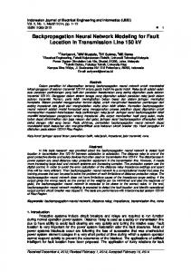
Introduction In neural network learning there are two general algorithm types [3,4] : - learning with teacher; - learning without teacher. In learning with teacher have to received/achieved a result, which is known and gives self- regulated direction to the neural network. The weight coefficients are as changed to achieve fixed by the teacher quantity. After its learning, the neural network has a test – only entry signals are submitted, without the signal which must be received. The concrete exit values are received on the network’s exit. The basic algorithm for neural network learning with teacher is “Back propagation “. It is developed for many-layered networks with straight transfer. The algorithm is applied in many-layered neural networks with straight transfer. Figure 1 shows in abbreviated notationof a classic tree-layered neural network.

P Rx 1 R

W1 S1x

b1

S1x

2

+

3

а1 W n F1 S1x S21x S1x 1 b S2x 1

+

2

n F2 S2x

а2 W 3 S2x S 3x 1 b S3x

+

3 n3 3 а F S3x S3x

Fig.1 In the many-layered networks, the one layer’s exits become entries for the next one. The equations describing this operation are:

61

a m + 1 = f m + 1( wm + 1.a m + b m + 1) for m=0.2,...,M-1,

(1)

where: ƒ M is the number of the layers in the network; ƒ am is the exit of the m-layer of the neural network; ƒ W is a matrix of the influence coefficients of the everyone of the entries; ƒ b is neuron’s entry bias; ƒ Fm is the transfer function of the m neural layer exit. The neuron in the first layer receives outside entries: а0=р. The neurons’ exits from the last layer determine the neural network’s exits: а= ам. Because it belongs to the learning with teacher methods, to the algorithm are submitted couple numbers (an entry value and an achieving aim – on the network’s exit) {p1, t1}, {p2 , t2}, ..., {pQ , tQ} (2) о ∈ (1...n) n – numbers of learning couple, where рQ is the entry value (on the network entry), and tQ is the exit’s value replying to the aim. Every network’s entry is preliminary established and constant, and the exit have to reply to the aim. The difference between the entry values and the aim is the error – e. The “back propagation” algorithm use least-quarter error. In learning the neural network, the algorithm recalculates network’s parameters (W and b) so to achieve least-square error. Application

Figure 2 shows the model describing the neural network learning with straight transfer by “Back propagation” method. Initially in the network there are the following main centers: ƒ In position SG - one αG- center has a characteristic “casual numbers generator for generalizing weight coefficients and neural network bias. ƒ Every position SF1, SF2 and SF3 – there is one αRi –center, i∈(1,2,3) having the characteristics “transfer functions of the I-layer from the neural network. ” ƒ In position St - one αt-center having the characteristic “learning aim of the neural network’s exit.” ƒ In position Sez - one αez-center having the preliminary fixed error for neural network’s learning. The generalized net is present by the set of transitions [1,2]:. А= { Z1, Z2, Z3, Z4, Z5, Z6 , Z7 }, where the transitions describe the following processes: Z1 – generalizing random vector for values of the weight matrix W and replacing b; 62

Rk

Z2 – calculating the sum of the entries’ influences n k = ∑ ( Pi .Wki ) + b k for k-network 2

i =1

layer, where: • • • •

RК – numbers of neurons in the k-neural layer; P – an entry network’s vector; W – matrix having weight influence coefficients for every signal and layer; b – bias the layers; Z2

Z1

Z3

SWb

Sa3

SWb SG

St

Sn

Z5

Z4

Z6

Se S51

Sez

SNW

SP1 SR1 SP2

SR2

SP3

SR3

SAWb

SF1 SF2 SF3

Z7

S71 S72 S73 S74 S75 S76

Figure 2

Z3 – calculating the exit аk=Fk(nk) from the k-network layer;

63

SA6 S52

Z4 – determining the difference between the received value (а3) and the fixed learning aim and the least square error between them; Z5 – determining is the neural network learnt or not; Z6 – calculating the new weight coefficients and neural network’s bias; Z7 – submitting the transfer functions for calculating the new weight coefficients, the neural network’s bias and for calculating the аk exit. GN – the model contents six transitions having the features: Z1 = R1=

SG

SWbN

SWb

SG

WG ,WbN

WG ,Wb

True

where: WG,WbN = “ Random vector for restoring W и b is generalized”; WG,Wb= “Random vector for calculating the network exit is generalized.” Z2=

SWb SP1

Sn False WP1,n

SAWb WWb,AWb False

S R1 S R2= R 2 SR 3

WR1,n WR 2,n WR 3,n

False False False

S NWb SP 2

False WP 2,n

WN Wb ,AWb False

SP 3 SAWb

WR 2,n True

False False

where: WP1,n =”The exits of the first neural layer having entry vector Р1 are calculated. ”; WR1,n = “ The exits of the first neural layer with R1 numbers of neurons in the first layer are calculated.”; WR2,n = “ The exits of the second neural layer with R2 numbers of neurons in the layer are calculated.”; WR3,n = “ The exits of the third neural layer with R3 numbers of neurons in the layer are calculated.”; WP2,n =”The exits of the second neural layer with entry vector Р2 are calculated.”; WP3,n =”The exits of the third neural layer with entry vector Р3 are calculated.”; WWb,AWb=”Arbitrarily generalized values of W and b are recorded/inscribed for layers exits’ calculating.” WNWb,AWb=”Recalculated values for W and b are recorded/inscribed for layers’ exits receiving.” 64

Z3= Sa 3

SP 2

SP 3

Sn

Wn ,a 3

Wn ,P 2

Wn ,P 3

R3= S71

False

W71,P 2

False

S72

False

False

W72,P 3

S73

W73,a 3

False

False

where: Wn,a3 = “The neural layer’s exit having sum “n” is defined.; W73,a3 = “ The neural network exit having transfer function F3 for the third neural layer is defined.” Wn,P2= “The first neural layer’s exit having sum “n” is defined.” W71,P2 = “The first neural layer’s exit having transfer function F1is defined.” Wn,P3= “The second neural layer’s exit having sum “n” is defined.” W72,P3 = “ The second neural layer’s exit having transfer function F2 is defined.” At the position Sа3 the centers receive a characteristic “exit of the neural network in entry P, weight coefficient, bias W and b, and transfer functions F.” Z4 = R4= Sa 3

Se Wa 3,e

St

Wt ,e

where: Wa3,e = “ The neural networks exit’s error in exit a3 is calculated.” Wt,e = “The neural network exit’s error in fixed aim t is calculated.” At the position Se like a characteristic the centers receive the value of the least square error in the network’s learning. Z5 = S51

S52

R5= Se

We,51

We,52

Sez

Wez,51

Wez ,52

where: Wе,51 = “at the received error the neural network is not learned enough.” Wеz,51 = “at the fixed error the neural network is not learned enough.” Wе,52 = “at the received error the neural network is learned.” Wеz,52 =“at the fixed error the neural network is learned.”

65

At position S51 the centers receive the value of the received error for recalculating the weight coefficients and bias. Z6 = S NWb

SA 6

SWb

False

WWb ,A 6

S51

W51,NWb

W51,A 6

R6= SAWb WAWb,NWb WAWb,A 6 S74

W74,NWb

W74,A 6

S75

W75,NWb

W75,A 6

S76

W76,NWb

W76,A 6

where: WWb,A6 = “In the archives are inscribed the initial values of W and b”; W51,NWb = “W(n+1) and b(n+1) are calculated with the previous values of W(n) and b(n) and the calculated error, and it is sent into the network”; W51,А6 = “W(n+1) and b(n+1) are calculated with the previous values of W(n) and b(n) and the calculated error, and it is sent into the archives”; WAWb,NWb = “Calculating W(n+1) and b(n+1) with the previous values of W(n) and b(n) from the archives, and it is sent to the network”; WAWb,А6 = “Calculating W(n+1) and b(n+1) with the previous values of W(n) and b(n) from the archives, and it is sent into the archives again”; W74,NWb =“W(n+1) and b(n+1) are calculated with the previous values of W(n) and b(n), transfer function F1 and the calculated error, and it is sent into the network”; W75,NWb =“W(n+1) and b(n+1) are calculated with the previous values of W(n) and b(n), transfer function F2 and the calculated error, and it is sent into the network”; W76,NWb =“ W(n+1) and b(n+1) are calculated with the previous values of W(n) and b(n), transfer function F3 and the calculated error, and it is sent into the network”; W74,А6 = “W(n+1) and b(n+1) are calculated with the previous values of W(n) and b(n), transfer function F1 and the calculated error, and it is sent into the archives”; W75,А6 = “W(n+1) and b(n+1) are calculated with the previous values of W(n) and b(n), transfer function F2 and the calculated error, and it is sent into the archives”; W76,А6 = “W(n+1) and b(n+1) are calculated with the previous values of W(n) and b(n), transfer function F3 and the calculated error, and it is sent into the archives”; Z7 =

R7=

SF1 SF 2 S F3

S71 S72 WF1,71 False False WF 2,72 False False

S73 S74 False WF1,74 False False WF3,73 False

S75 S76 False False WF 2,75 False False WF3, 76 66

where: WF1,71=”The function F1 is submitted for calculating the exit of the neural network.” WF2,72=” The function F2 is submitted for calculating the exit of the neural network.” WF3,73=” The function F3 is submitted for calculating the exit of the neural network.” WF1,74=” The function F1 is submitted for calculating the new weight coefficients and bias” WF2,75=” The function F2 is submitted for calculating the new weight coefficients and bias” WF3,76=” The function Функцията F3 is submitted for calculating the new weight coefficients and bias” Conclusion

This model introduces the working method of the neural network with straight propagation and its learning using the algorithm of “Back propagation”. About constructing a model of information processes in described structure there are used generalized nets because they offer powerful implement for modeling the parallel process and they allow their stimulation and following their behavior in future, their managing and optimization. Reference

[1] Atanassov, K. Generalized Nets, World Scientific. Singapore, New Jersey, London, 1991. [2] Atanassov, Kr., Introduction in the theory of the generalized nets, Pontika-Print, Bourgas, 1992. [3] Haykin, S, Neural network and comprehensive foundation, Prentice Hall, New Jersey, 1999. [4] Howard Demuth, Mark Beale, Neural network design, Prentice hall, New Jersey, 1995. [5] Atanasov Kr. , E. Sotirova, On global Operator G21 defined over Generalized Nets, Cybernetics and information technologies, Volume 4 No 2, Bulgarian Academy of Science, Sofia, 2004.

67