Improving the Quality of Random Number Generators by Applying a ...
Recommend Documents
Dec 21, 2010 - Email: [email protected], [email protected], [email protected]. AbstractâIn ... random number generator; Statistical tests; Internet security; ..... http://stat.fsu.edu/ geo/diehard.html, 1996.
Lottery. ⢠Applications of Random Numbers. ⢠Pseudo Randomness VS. True Randomness ... Quantum Random Number Generator (QRNG). Time of arrival.
dictates the use of RNGs based on free running oscillators (FRO) whose ran- ...... Time-random photons fall onto the single photon detector consisting of a.
program at the University of Minnesota - Twin Cities. This research ... The Art of
Computer Programming by D. E. Knuth (second edition, 1981). My project shifted
...
Oct 21, 2016 - random numbers on demand (ANU, 2016; Humboldt-. Universität, 2016 .... be accessed from the software inside the computer or cre-.
Random Generator Quality Assessment Luizi, Cruz, & van de Graaf. Assessing the ... E-mail: [email protected] Phone: +55 31. 3409 5929. Fax: +55 31 .... template length = 9. 9 Overlapping Templates Matching Test parametric template length = 9 ..... â
on uniform random number generation for stochas- ... Without a good random number generator (RNG), ... ture of the RNG and view the un as random vari-.
Jun 22, 2013 - 3 See, for example, âIntel Corporation Intel 810 Chipset Design Guide,â. June 1999 ... 'Nehemiah' Random. Number ...... success. [1] N. Meteopolis and S. Ulam, Journal of the American Statistical Association, 44, 335 (1949).
is theoretically unbreakableâone-time pad [2]. This cipher. Manuscript received January 7, 2000; revised September 17, 2000. This work was supported in part ...
The implications of the refutation of the IMMI hypothesis especially on associated phenomena are also discussed. Keywords Meta-analysis; Psychology; random ...
address these questions and provide a state-of-the-art overview of F2-linear .....
reason in the previous subsection: efficient jumping-ahead is easier for a ......
editors, Computational Science and its Applications—ICCSA 2003, volume 2667.
margin L. For larger jq1 01j, the map becomes increasingly asymmet- rical and the difference in probabilities of 0s and 1s increases. It is possible that a local ...
Luis L BonillaEmail author; Mariano Alvaro; Manuel Carretero. Luis L Bonilla. 1 ... First Online: 29 June 2016. Received: 28 ... Keywords. random bit generator semiconductor superlattice deterministic and stochastic chaos ...... NIST Statistical Test
Biological random seeds could also be applied to key generation for electronic signatures used by subscribers. Random number generators (RNG) can be imple ...
Oct 4, 2012 - statistical properties of a random sequence - like the equiprobability of all numbers ... the example, the increase of the world human population.
RNG based on a chaotic map can be analyzed. Concluding re- marks are given in Section IV. II. CHAOS AND RNGS. Theory of chaos, as a branch of theory of ...
Email:{jacques.bahi, xiaole.fang, christophe.guyeux, qianxue.wang}@univ-fcomte.fr ... generator based on chaotic iterations which behaves chaotically as defined by Devaney. ...... Overlapping Template Matching Test is the number of.
Most digital signature algorithms rely on random sources which stability and quality crucially influence security: a typical example is El-Gamal's scheme [9].
GEORGE S. FISHMAN. Abstract. This paper presents the results of a search to
find optimal maximal period multipliers for multiplicative congruential random ...
Mar 24, 2005 - the Mersenne-Twister âMT1937â proposed by Matsumoto and Nishimura (1998). For more details see eg the reviews by Deng (1998), ...
Mar 4, 2010 - called Arithmetic Logic Units (ALUs), that are grouped into ...... [24] A. M. Ferrenberg, D. P. Landau, and Y. J. Wong, âMonte Carlo simulations: ...
gures of merit do worse in the tests than those with a not-so-good gure of merit. .... A list of MRGs of di erent sizes, good with respect to a related criterion (the ... We believe that they constitute excellent choices for general- purpose statisti
and motivate our sponge-based construction in Section 3. We discuss ...... Keccak is a family of sponge functions submitted to the SHA-3 contest or- ganized by ...
Feb 1, 2007 - Yet jumping ahead for F2-linear generators of large order k (such as the Mersenne twister) remains slow with this method. One way to make the ...
Improving the Quality of Random Number Generators by Applying a ...
Dec 21, 2016 - ââCorresponding author. Email addresses: [email protected] (Michael Kolonko), ... A random number generator (RNG for short) is an algorithm that pro- ...... testu01/tu01.html, accessed: 2015-10-05 (Aug. 2009).
Improving the Quality of Random Number Generators by Applying a Simple Ratio Transformation
arXiv:1612.07318v1 [cs.OH] 21 Dec 2016
Michael Kolonkoa,∗∗, Zijun Wub,∗, Feng Gua a
Institut für Angewandte Stochastik und Operations Research, Technical University of Clausthal, Erzstr. 1, D-38678 Clausthal-Zellerfeld, Germany b Beijing Institute for Scientific and Engineering Computing, School of Applied Mathematics and Physics, Beijing University of Technology, Pingleyuan 100, 100124, Chaoyang, Beijing, China
Abstract It is well-known that the quality of random number generators can often be improved by combining several generators, e.g. by summing or subtracting their results. In this paper we investigate the ratio of two random number generators as an alternative approach: the smaller of two input random numbers is divided by the larger, resulting in a rational number from [0, 1]. We investigate theoretical properties of this approach and show that it yields a good approximation to the ideal uniform distribution. To evaluate the empirical properties we use the well-known test suite TestU01. We apply the ratio transformation to moderately bad generators, i.e. those that failed up to 40% of the tests from the test battery Crush of TestU01. We show that more than half of them turn into very good generators that pass all tests of Crush and BigCrush from TestU01 when the ratio transformation is applied. In particular, generators based on linear operations seem to benefit from the ratio, as this breaks up some of the unwanted regularities in the input sequences. Thus the additional effort to produce a second random number and to calculate the ratio allows to increase the quality of available random number generators. ∗
Preprint submitted to Mathematics and Computers in Simulation
December 23, 2016
Keywords: random number generation, combination of random generators, ratio of uniform random variables, empirical testing of random generators 1. Introduction Stochastic simulation is an important tool to study the behavior of complex stochastic systems that cannot be mathematically analyzed, as it is often the case e.g. in network models for traffic, communication or production. The basis of these simulation tools is a (pseudo-) random input provided by a random number generator. A random number generator (RNG for short) is an algorithm that produces sequences of numbers that, viewed as an observation of a random experiment, can be modeled mathematically by a sequence of independent, identically distributed random variables (i.i.d. rvs). As basis for most simulations, these rvs should have the uniform distribution U (0, 1) on the interval [0, 1]. Of course, a deterministic algorithm can only approximate this mathematical model. Its deviance from the model is used to measure the quality of the generator. A lot of investigations have been made into that direction for different types of generators proposed over time, see e.g. [1] or [2] for a survey. In particular, a large number of empirical tests have been developed to assess the quality of RNGs. In this paper we are going to show that one can transform many simple, moderately good generators into statistically excellent ones using the ratio of their output. We show this with the test suite TestU01 from [3], which has become a standard for RNG testing. A general framework for RNGs producing numbers in the interval [0, 1] is described in [4]. It consists of a finite set S of internal states, a function f : S → S describing the recursion, a seed state s0 and an evaluation function g : S → [0, 1]. Starting with the seed state s0 , a sequence of states (si )i≥0 is constructed using the recursion si+1 := f (si ), i ≥ 0. The random numbers returned are ui := g(si ), i ≥ 0. Well-known examples for RNGs are the linear congruential generators (LCG) of order 1. Here, f (s) := (as + c) mod M for some constants a, c, M ∈ N and S := {0, 1, . . . , M − 1}. The integers s that serve as internal states are turned into output values from [0, 1] by the evaluation function g(s) := s/M . 2
In many popular generators the internal state consists of one or more integers from a bounded set NM := {0, 1, . . . , M − 1}. The evaluation step then selects one of these integers and divides it by M as in the example above. This is the case e.g. in LCGs of higher order, in many so-called Lagged Fibonacci generators and more complex combinations of RNGs as given in [1], [5], [6] or [7]. This way of producing random numbers from [0, 1] using a division by a constant M will be referred to in the sequel as the direct approach. In this paper, we assume that we are given a RNG that internally produces integers xi ∈ NM as above, but the final evaluation step is a more complex transformation that uses two consecutive values x2i , x2i+1 ∈ NM and returns ui :=
min{x2i , x2i+1 } max{x2i , x2i+1 }
(1)
where the cases x2i · x2i+1 = 0 and x2i = x2i+1 will be considered in detail in Subsection 2.1. We shall call (1) the ratio transformation and x1 , x2 , . . . its input sequence from the base RNG. To our knowledge, this type of ratio transformation was first used in [8]. To make the comparison between the ratio transformation and the direct approach fairer, we will consider an extension of this approach that also uses two random numbers and returns x2i x2i+1 + . wi := M M2 We call this the direct-2 approach. Note that our ratio transformation is computationally slightly more complex than direct-2. We start the paper with a theoretical analysis of the ratio transformation. We show that the cumulative distribution function (cdf) of the ratio transformation of two independent discrete random variables X1 , X2 , that are both uniformly distributed over NM , approximates the continuous uniform distribution on [0, 1]. This approximation, though not as close as by the direct approaches, yields values that are much less regularly distributed than those from the direct approaches. We believe that this is the reason for the superior empirical behaviour. The empirical quality of the ratio transformation is tested using the standard test batteries Crush and BigCrush from [2]. Typically, simple RNGs fail many of these tests with the direct approach. However, if the ratio transformation is applied, the number of tests failed is reduced considerably. In 3
particular, we tested the RNGs from [2] that failed up to 40% of the 144 tests of Crush. When the ratio transformation is applied to their output, about half of them passed all tests of Crush, whereas an application of the direct-2 approach could hardly improve their performance. This shows that the ratio transformation is able to turn simple, moderately good RNGs into excellent ones. First observations in that direction were reported in [8]. The paper is organized as follows: in Section 2, we investigate theoretical properties of (1) under the assumption that the inputs are from ideal RNGs. In Section 3 we report on empirical tests with the Crush/BigCrush test battery from [2] with different types of base RNGs, each time comparing the direct approaches with the ratio transformation. Finally, we give a short conclusion. 2. The Mathematical Model 2.1. The Cumulative Distribution Function of the Ratio Transformation In this Section we investigate the mathematical model of the ratio (1) where we replace the input sequence by random variables with a uniform distribution. We prove that the ratio transformation preserves uniformity at least approximately. For completeness, we first give a simple theorem which states that the ratio of two continuous U (0, 1)-distributed independent random variables is again U (0, 1)-distributed. Then, we will study the more complicated situation where the input is from a discrete uniform distribution. Note that for a continuous random variable U with distribution U (0, 1), its cdf is FU (t) = P(U ≤ t) = t and its density fU (t) = 1 for t ∈ [0, 1]. Theorem 1. Let U1 , U2 be two independent and identically distributed random variables with distribution U (0, 1) and define the ratio Z := where we put
0 0
min{U1 , U2 } max{U1 , U2 }
(2)
= 0. Then Z has distribution U (0, 1), too.
Proof. As P(U1 · U2 = 0) = P(U1 = U2 ) = 0 we may exclude these two cases and obtain P(Z ≤ t) = P(
min{U1 , U2 } ≤ t) = 2P(0 < U1 ≤ tU2 ) max{U1 , U2 } 4
Z
1
Z
1
P(U1 ≤ tu) du = 2
=2
tu du = 2t/2 = t, 0
0
for all t ∈ [0, 1]. Now we assume that the input is from two i.i.d. random variables X1 , X2 with the discrete uniform distribution U (NM ) on NM = {0, 1, . . . , M − 1}, i.e. 1 P(X1 = k, X2 = l) = 2 for all k, l ∈ NM . (3) M Then, we have P(X1 · X2 = 0) ≈ 2/M and P(X1 = X2 > 0) ≈ 1/M. A straightforward extension of the ratio (1) would choose 0 as return value in case X1 · X2 = 0 and return value 1 if X1 = X2 > 0, see [8]. As it is a common practice with RNGs to completely avoid 0, 1 as return values, we introduce two replacement values ε0 and ε1 with 0 < ε0 < 1 − ε1 < 1, and let them appear with almost equal small probability (≈ 1.5/M ). We therefore define M − 1 + bM/2c 2M 2 2M − 1 − bM/2c ε1 := 2M 2
ε0 :=
(4)
where bac is the largest integer less or equal a ∈ R. Note that 0 < ε0 , ε1 < 1/(M − 1) and that for large M, ε0 ≈ ε1 ≈ 0.75/M . The motivation for this particular choice will become clear from Theorem 3 below. In the sequel we will use the following ratio transformation of two inputs x1 , x2 ∈ NM if x1 = 0 < x2 or 0 ≤ x1 = x2 ≤ bM/2c − 1, ε 0 min{x1 ,x2 } h(x1 , x2 ) := max{x1 ,x2 } if x1 · x2 > 0 and x1 6= x2 , 1 − ε1 if x2 = 0 < x1 or x1 = x2 ≥ bM/2c, (5) i.e. we split the cases x1 · x2 = 0 and x1 = x2 more or less evenly between the two values ε0 and 1 − ε1 . The next Theorem gives the cdf of the discrete random variable h(X1 , X2 ). We show in Theorem 3 that this is a close approximation of the cdf of U (0, 1).
5
Theorem 2. Let X1 , X2 be i.i.d. U (NM )-distributed random variables and Y = h(X1 , X2 ). Then the cdf of Y is given by 0 2ε 0 P(Y ≤ t) = 2ε0 + 1
2 M2
·
PM −1 k=1
btkc
if if if if
0 ≤ t < ε0 ε0 ≤ t < M1−1 1 ≤ t < 1 − ε1 M −1 1 − ε1 ≤ t ≤ 1
(6)
min{X1 ,X2 } may attain is M1−1 and Proof. The smallest nonzero value that max{X 1 ,X2 } −2 similarly, M = 1 − M1−1 is the largest value smaller than 1. We have 0 < M −1 −2 ε0 < M1−1 and M < 1 − ε1 . Therefore, using (3) M −1
M −1 2 X P(X2 = k)P(X1 ≤ kt) = 2ε0 + 2 btkc, M k=1
here t < 1 implies X1 6= X2 , which proves the Theorem.
6
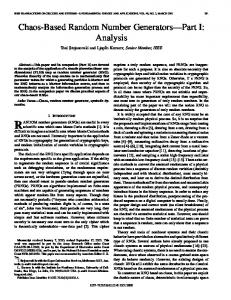
2.2. The Deviation of Y from the Uniform Distribution We want to measure the quality of the ratio transformation Y by the maximal deviation of its cdf FY (t) := P(Y ≤ t) as given in Theorem 2 from the cdf of a U (0, 1)-distributed random variable U with FU (t) = t, t ∈ [0, 1]. This difference ∆Y := sup |FY (t) − t| t∈[0,1]
0.2
0.4
0.6
0.8
1.0
is also called Kolmogoroff-Smirnov-distance (KS-distance).
0.0
P(Y ti − hence ti −
1 k
1 m 1 mj − 1 = − = ∈ D ∪ {0}, k n nj nj
≤ ti−1 and 1 bti−1 kc ≥ b(ti − )kc = bti kc − 1. k
For the second case of (18), we have bti kc < ti k as k 6= nj. Assume ti−1 k < bti kc, then bti−1 kc ≤ ti−1 k < bti kc < ti k