2004-01-0110
In-Cylinder CFD Simulation Using a C++ Object-Oriented Toolkit Hrvoje Jasak∗ and Henry G. Weller Nabla Ltd, United Kingdom
Niklas Nordin† Chalmers University of Technology, Sweden
ABSTRACT
Moreover, injected fuel sprays often impinge onto engine wall, raising issue to yet another set of modelling, including spray-wall interaction and wall films, together with the associated heat, mass and momentum transfer. From the geometrical point of view, the situation is similarly complex: an IC engine is a 3-D geometry of complex shape and contains a moving piston and valves as well as stationary combustion deck and manifolds. In order to accommodate the motion of engine components, computational mesh undergoes both geometrical (mesh motion) and topological changes. Typically, a task of building a mesh of reasonable quality for the complete IC engine cycle and defining the motion may take several weeks. In order to perform a successful flow simulation in an IC engine, the range of models listed above needs to take into account the effects of mesh motion and topological changes. The consequence of these stringent requirements is that a number of CFD codes capable of tackling IC engine modelling is very small indeed. In a research environment it is often necessary to implement and test new physical models. Model implementation needs to handle the complexities of mesh motion and topological changes on unstructured 3-D meshes and at the same time be simple and errorfree. As the models and the underlying numerics become more complex, the probability of introducing implementation or model-to-model interaction errors increases rapidly. The objective of the work presented in this paper is to create a software environment where it is possible to implement new models, refine the existing ones and experiment with model combinations easily and reliably. At the same time, we aim to satisfy the mesh handling requirements and simplify the setup as much as possible. Our first task is to establish a way of representing and reliably implementing new physical models in software. Secondly, numerical support for all relevant
Successful simulation of fluid flow, heat transfer, fuel injection and combustion in internal combustion engines involves a spectrum of physical models operating in a complex 3-D geometry with moving boundaries. The models are formulated in the Eulerian and Lagrangian framework and interact in complex ways. In this paper, we present FOAM, an object-oriented software toolkit designed to facilitate research in physical modelling by separating the handling of physics from numerical discretisation techniques. This is achieved by mimicking in the code the continuum mechanics equations of the physical model. Complex mesh handling, choice of numerics and the simulation efficiency are handled transparently. Capabilities of the toolkit are demonstrated on two in-cylinder combustion simulations.
INTRODUCTION CFD simulation of in-cylinder flows in Internal Combustion (IC) engines is demanding both in terms of physical modelling and geometrical mesh handling. From the modelling standpoint, the physical phenomena of interest span a wide spectrum. At the low end of requirements, compressible turbulent flow of a Newtonian fluid is simulated (cold-flow simulation) and the model may then be successively extended to include heat transfer, combustion, chemical kinetics, modelling of fuel sprays, which includes spray injection, atomisation, turbulence dispersion, drop breakup and collision and the interphase exchange of mass, momentum and energy [1] etc. ∗ Corresponding author, The Mews, Picketts Lodge, Picketts Lane, Salfords, Surrey RH1 5RG, United Kingdom, Email:
[email protected], Tel: +44 (0)1293 821 272 † Dept. of Thermo and Fluid Dynamics, Chalmers University of Technology, Sweden, E-mail:
[email protected]
1
modelling frameworks present in IC engine simulations should be provided. Thirdly, the issues of mesh handling should be considered, including mesh generation, motion and topological changes. Finally, we need to address the efficiency concerns of the new design and illustrate the performance of the software on real engine simulations. In this paper, we present FOAM (Field Operation And Manipulation) [2], an object-oriented numerical simulation toolkit specifically tailored for simple implementation of physical models in continuum mechanics. The toolkit implements operator-based implicit and explicit second- and fourth-order Finite Volume (FV) discretisation in 3-D and on curved surfaces, a second order FEM solver and a particle tracking model. Flexibility in mesh handling is provided by supporting unstructured polyhedral meshes and topological changes. Efficiency of execution is achieved by the use of preconditioned Conjugate Gradient and Algebraic Multigrid solvers and the use of massively parallel computers in the domain decomposition mode. Automatic mesh motion solver, where point motion is defined by only prescribing the boundary motion, facilitates the setup of deforming mesh simulations. The rest of the paper will be organised as follows. We shall first examine model representation in the Eulerian framework, defining a set of objects needed for this purpose and classes that represent them in software. Object-oriented design brings interesting implications in terms of code granularity and re-use, which will also be examined. Important and illustrative interaction between basic classes will be presented graphically, using the Unified Modelling Language (UML), [3]. This is followed by the description of mesh handling suitable for complex geometries and topological mesh changes. A novel way of performing automatic mesh motion based exclusively on prescribed boundary motion will be described. A short review of the Lagrangian particle tracking and the Diesel spray model implementation will also be given. The paper is concluded with some efficiency considerations and two numerical examples of in-cylinder combustion simulations.
tered throughout the software. This approach leads to possible coding/implementation errors as well as testing and maintenance concerns. Thus, model implementation is in most cases a highly skilled job, requiring not only detailed knowledge of the physics and numerics but also of the software in which the model is implemented. The natural language of model representation in continuum mechanics is the language of partial differential equations. Therefore, model implementation could be made easier if we could tailor the code representing the model to look like the partial differential equation it implements. As an example, our aim is to translate the mathematical expression · ¸2 1 ∂k +∇•(u k)−∇•[(ν + νt )∇k] = νt (∇u + ∇uT ) −² ∂t 2 (1) into the following software implementation (this is valid C++ syntax): solve ( fvm::ddt(k) + fvm::div(phi, k) - fvm::laplacian(turb.nu() + nut, k) == nut*magSqr(symm(fvc::grad(U))) - fvm::Sp(epsilon/k, k) ); If this is accomplished, the model structure, its implementation and inter-equation coupling could be examined independently from the related numerical issues. Also, substantial code re-use could be achieved: it is likely that a large number of models would share the same source code implementation of various terms, thus eliminating the likelihood of coding errors. Let us now consider the steps necessary to convert Eqn. (1) into the software quoted above. Continuum mechanics operates on fields of scalars, vectors and tensors defined on a domain in time and space. Therefore, we first need a representation of tensors of different rank and the associated tensor algebra. In order to define a tensor field, we also need to represent space and time. A computational mesh discretises the space as a set of locations where the variables are stored, a set of points and the elements/cells supported by the points. Additionally, the external boundary of the mesh consists of a number of boundary faces. The temporal dimension is discretised by splitting the time interval into a finite number of time-steps. Numerical methods represent tensor fields as lists of values on pre-defined locations in the mesh, together with an interpolation function between the storage points. We can now also define the differential operators on tensor fields: divergence, gradient, curl and the temporal derivative; the actual implementation depends on the particular discretisation method.
MODEL REPRESENTATION Of the two modelling frameworks, Eulerian frame models seem more challenging in terms of software representation. Here, models are described as sets of coupled partial differential equations with the terms falling into several categories: the temporal derivative, convective and diffusive transport and various source and sink terms. In most CFD codes, implementation of a new model implies that the code which discretises the terms in the equation is repeated in a form already present elsewhere and updates resulting from model-to-model interaction and boundary condition handling are scat2
An important part of problem definition are the initial and boundary conditions. Initial conditions can already be described in this framework, but boundary conditions require further consideration. The boundary is first split into patches according to the condition to be enforced. Patch values and the specification of the boundary condition is given on a per patch basis. Numerical machinery described so far allows us to assemble an explicit solver for Eqn. (1); for implicit discretisation some additional components are needed. Implicit discretisation converts the original partial differential equation into a linear algebraic equation: X a N kN = r P , (2) a P kP +
objects inferred from Eqn. (1), we can now review their software implementation in FOAM. The implementation of tensor algebra is based on the VectorSpace class, which automatically expands the algebraic operations between tensors of different rank, including the inner and outer products. The spatial domain is represented in two levels. The generic mesh engine, polyMesh, handles a mesh of arbitrary polyhedra bounded by arbitrary polygons. polyMesh also handles point motion and topological changes (morphing). Other parts of the software can access but not change the mesh data (cell volumes, connectivity etc.) using the public interface of the polyMesh class which protects the data from accidental corruption. The information available in polyMesh is not necessarily presented in a way appropriate for use in discretisation. The fvMesh class packs the data for convenient usage in the FV discretisation; for the FEM solver, the femMesh class serves the same purpose. fvMesh also holds the sparse matrix addressing object (dictated by the mesh) and supports cell-to-face interpolation. Class derivation and collaboration diagram for the fvMesh class is graphically represented in Fig. 1 using UML. In short, a box represents a class, a solid arrow stands for public inheritance (“is-a” relation) and a dashed arrow indicates usage (“has-a” relation), with the edge of the arrow labelled with the variable responsible for relationship.
N
with one equation assembled for each computational point. Here, kP is the value in the chosen computational point which depends on the values in neighbouring locations kN , creating a matrix equation: [A] [k] = [r],
(3)
where [A] is a sparse matrix, [k] is the vector of ks for all computational points and [r] is the right-hand side vector. Therefore, we need to represent a sparse matrix (including matrix coefficients and addressing pattern), matrix calculus and provide linear equation solvers. Considering Eqn. (1) from the discretisation standpoint, one can state that it represents a sum of several operators (temporal derivative, convection term, diffusion term, source/sink terms), each of which can separately be transformed into a linear equation through discretisation. Eqn. (2) is then assembled by summing up the individual equations and assembled into a matrix equation for all points, Eqn. (3).
polyMesh
lduAddressingFvMesh lduPtr_
fvMesh mesh_
OBJECT-ORIENTED FRAMEWORK AND C++
surfaceInterpolation
mesh_
boundary_
fvBoundaryMesh
Figure 1: UML diagram for the fvMesh class.
Object-oriented framework allows the software designer to create a more manageable software, with lower maintenance cost, extensive code re-use, fewer bugs and easier extendibility. The leading object-oriented language today is C++ [4, 5]. Written as a “better C”, it provides not only the support for object orientation and generic programming but also offers near-universal availability and efficiency needed for scientific computations. The main features of the language are data abstraction, allowing the designer to introduce new data types appropriate for the problem, object orientation, i.e. bundling of data and operations into classes, protecting the data from accidental corruption and the creating class hierarchies, operator overloading, which provides natural syntax for newly defined classes and generic programming, allowing code re-use for equivalent operations on different types. Having recognised the basic
The temporal dimension of the simulation is handled by the time class, integrated into the data-handling system (database), which is also responsible for data input/output, simulation control updates etc. A GeometricField class, Fig. 2, is a software representation of a tensor field and consists of an internal field, holding a list of values of appropriate tensor rank for all computational points and a boundary field. Some auxiliary data, most notably the dimension set, is also present. A GeometricBoundaryField is a list of patch fields (one for each patch), each of which holds the field values for the patch and the boundary condition. A patch field also handles the discretisation-specific issues related to the implementation of boundary conditions and updates 3
refCount
IOobject
Istream
FieldField< PatchField, Type >
List< Type >
Field< Type >
isPtr_
regIOobject
GeometricBoundaryField boundaryField_
dimensionSet dimensions_
GeometricField
Figure 2: UML diagram for the GeometricField class.
the boundary values. Boundary condition handling is done through a virtual mechanism, where a generic interface (shared by all boundary conditions) is defined and specific boundary conditions implement this interface. The basic boundary conditions are fixedValue, zeroGradient, mixed, symmetryPlane, coupled etc. More complex boundary conditions are implemented by combining and expanding the base types. In this way, the implementation of a boundary condition is localised to its class; introduction of new boundary conditions requires no modifications elsewhere in the code. For implicitly updated conditions, such as cyclic and processorto-processor boundaries, a lduCoupledInterface class provides a wider interface and is automatically updated in matrix operations.
on this level is independent of discretisation.
IMPLEMENTING THE FV DISCRETISATION Let us consider the implementation of the FVM in this context. The role of FV discretisation is two-fold. The explicit FV calculus (fvc) implements the differential operators fvc::div, fvc::grad, fvc::curl etc., creating a field. The implicit FV method (fvm) converts expressions like fvm::ddt(k) into matrix coefficients, which is a straightforward discretisation task. Currently, the following set of implicit operators is available (names are self-explanatory): fvm:ddt, fvm::d2dt2, fvm::div, fvm::laplacian. For completeness, explicit equivalents of the implicit operators are also implemented. Additionally, implicit handling of source terms is performed by the fvm::Sp and fvm::SuSp operators; the explicit sources are added directly into [r] in the matrix equation. Imposition of boundary conditions on the matrix depends on the kind of discretisation that is being used: for example, the Dirichlet boundary condition effects the matrix in a different way for the FVM and FEM. It is therefore necessary to implement the FV-specific versions of boundary conditions. A sample UML diagram for the fvPatchField which implements boundary condition handling for the FVM is shown in Fig. 3. Specific boundary conditions (zeroGradientFvPatchField, fixedValueFvPatchField, etc) are then derived from the fvPatchField class. The discretisation-specific version of the matrix, fvMatrix, is derived from lduMatrix and handles the fvPatchField interface. This completes the implementation of the FVM. An interesting feature of this design is that the amount of code needed for a new discretisation method is relatively low. It consists of a class packing the mesh data, a generic interface for handling the boundary con-
A GeometricField can be defined on different sets of mesh objects (points, edges, faces, cells) and with different tensor ranks (scalar, vector, tensor etc.). This is a good example of generic programming, as the field functionality and algebra is independent of the rank or storage location and all fields share the same implementation. Operator discretisation produces a sparse matrix, represented by the lduMatrix class, which also implements the associated matrix algebra and linear equation solvers. The lduMatrix contains the diagonal, offdiagonal and coupling matrix coefficients. In order to avoid data duplication, its sparse addressing pattern is provided by the appropriate mesh class. Looking at Eqn. (1) and its implementation in the code, it now becomes clear how the system operates: on the l.h.s. the operators (ddt, div, and laplacian) create matrices, which are then summed up. On the r.h.s., the field calculus is used to create the source term to be added to the matrix diagonal or source vector [r]. As the final matrix is assembled, the individual terms are dimension-checked. Before calling the solver, the boundary conditions on k are enforced; the result of the solution is placed into k. Note that model representation 4
UList< Type >
List
geometricPatch
polyBoundaryMesh
< Type >
refCount
List< Type >
boundaryMesh_
polyPatch
fvBoundaryMesh polyPatch_
Field< Type >
lduCoupledInterface
boundaryMesh_
fvPatch
boundary_
mesh_
fvMesh
patch_
fvPatchField
Figure 3: UML diagram for the fvPatchField class.
ditions, a derived matrix class to enforce them on the matrix and the implementation of the actual discretisation operators. All other code is re-used with no changes. More importantly, the implementation of implicit operators for each method can be tested in isolation, is shared between various equations and, through generic programming, it is even shared between scalars, vectors and tensors of different rank.
quired that no tetrahedron is inverted, thus preventing degeneration of faces and cells. Secondly, bounded discretisation of the motion equation guarantees that the boundedness in the differential form is preserved when the equation is solved numerically. The advantage of automatic mesh motion lies in the fact that it is no longer necessary to prescribe the motion of all points in advance. The problem setup becomes simpler and may include solution-dependent motion. In IC engines, the engineMesh class provides information on piston and valve position; based on the boundary motion, the point position is solved for in every time step as a part of the simulation. Topological Changes. In extreme cases of boundary deformation, mesh quality can only by preserved by changing the number of cells in the mesh. A topological change is any mesh operation which changes the connectivity of the mesh or the number of points, faces or cells in it. Topological changes typically used in IC engine simulations are attach/detach boundaries, cell layer addition/removal and sliding mesh interfaces. Mesh operations requiring topological changes will be collectively termed mesh modifiers. Following the object-oriented approach, we first define a generic interface which supports primitive morphing operations: add/modify/remove a point, a face or a cell. Based on this set, topological operations mentioned above are implemented and all others may be supported. Thus, a polyMeshModifier is a virtual base class which operates in terms of primitive morphing operations and includes the triggering of topological changes based on some built-in criteria, e.g. cell layer thickness for cell addition/removal. The UML diagram for a sample mesh modifier, layerAdditionRemoval, is shown in Fig. 4. A layerAdditionRemoval modifier is specified by a set of oriented faces defining the base layer and the thickness threshold for layer addition and removal. Fig. 5 shows layer addition in action during valve opening; note the additional cell layers on the valve curtain. Topological changes required during the simulation
UNSTRUCTURED MESH HANDLING In order to take full advantage of simple model implementation, the toolkit also needs to handle complex geometries. The polyMesh class operates on the unstructured polyhedral mesh format [6], removing most constraints on mesh generation and allowing uniform and efficient treatment of all cell types, from tetrahedra and hexahedra to arbitrary polyhedra. A mesh is defined as a list of points, a list of polygonal faces in terms of point labels and a list of faces per cell. In order to perform IC engine simulations, we need to tackle two more issues: mesh motion and topological changes. Automatic Mesh Motion. IC engine simulations involve moving boundaries which need to be accommodated during the run. While the motion is defined solely on the boundary points, most CFD codes require the user to specify the motion of all points in the mesh. In practice, this is quite limiting, as it becomes difficult to prescribe solution-dependent motion or perform mesh motion on dynamically adapting meshes. Automatic mesh motion module implemented in the toolkit uses a second-order FEM solver to solve the mesh motion equation [7]. Here, the position of internal points is determined from the prescribed boundary motion such that an initially valid mesh remains valid. This is achieved in two ways. Firstly, polyhedral cells are implicitly subdivided into tetrahedra and it is re5
polyMeshMorphEngine
word
morphEngine_
null
name_ faceZoneName_
polyMeshModifier
List< label > pointsToCollapsePtr_ facesToCollapsePtr_
layerAdditionRemoval
Figure 4: UML diagram for the layerAdditionRemoval class.
other. From the implementation point of view, this is much easier to handle than the Eulerian framework.
MODEL LIBRARIES AND RUN-TIME SELECTION The basic blocks presented above are sufficient to create a code for IC engine simulations: 3-D FVM is used for Eulerian modelling of flow equations, turbulence, heat and mass transfer and combustion, Diesel spray is modelled using Lagrangian particle tracking and wall film can be handled by the 2-D FVM on wall surfaces. Unstructured mesh engine uses automatic mesh motion and topological modifiers to handle the motion/morphing needed for the run. Our concern at this point is three-fold. Firstly, a typical user is not interested in writing the complete simulation code based on the building blocks but rather in testing different combinations of models or implementing new sub-models. Secondly, the size of the top-level code would still be substantial and may be difficult to manage. Ideally, model implementation should be separated, encapsulated and re-usable. Finally, it is necessary to ensure that all new models are smoothly integrated into the top-level code and that their efficiency corresponds to the “built-in” functionality. To address the above concerns, FOAM provides a set of top-level libraries which are used in applications or in other libraries. A top-level library contains a set of models for the same purpose which answer to the same interface; examples are the Reynolds-averaged (RANS) turbulence model library, containing linear and nonlinear k−² and Reynolds stress models; transport model library, implementing various viscosity laws; Large Eddy Simulation (LES) sub-grid scale models; thermophysical models library, implementing various equations of state etc. The top-level code couples the libraries into a flow solver, implementing the flow and heat transfer equations. The model selection from a library is done at run-time. New models can be added to the appropriate model table at link-time and become available in the same manner as the supplied models. In fact, there is
Figure 5: Example of layer addition above the opening valve in the intake manifold.
are handled by the polyMeshMorphEngine, which contains a list of mesh modifiers, triggers the morphing operations and handles mapping of field data.
LAGRANGIAN MODELLING The base of the Lagrangian particle tracking model is the particle class, which records the position and location (cell or boundary face) of a particle within the mesh. A cloud is a set of particles with a reference to a mesh and the capability of adding, deleting and tracking particles. The UML diagram for the cloud class is shown in Fig. 6. The spray class uses basic tracking capabilities of a cloud on a parcel. A parcel class is a particle which carries the data about the population of droplets associated with it and handles heat, mass and momentum transfer with the continuous phase. Each parcel carries the set of properties of interest, e.g. droplet diameter, number of droplets in the population, droplet temperature etc. The spray class also contains the sub-models handling atomisation, drag, evaporation, heat transfer, breakup, collision and dispersion, executes the necessary sub-models on all parcels and performs data handling operations. In Lagrangian modelling, the sub-models are implemented in terms of interaction between a parcel and its surroundings or two parcels considered close to each 6
Field< vector > oldPointsPtr_
polyMesh allFaceCentres_ points_ regIOobject
mesh_
polyMesh_
IDLList< particleType >
pointMesh
pointMesh_
UList< label > neighbour_ owner_
Cloud
Figure 6: UML diagram for the cloud class.
no difference in the implementation of a new model by the end-user or a library developer. The principle of dynamic tables and run-time selection is used widely throughout the toolkit. For example, the selection of linear equation solvers, convection, diffusion, gradient discretisation (within the FVM) etc. is performed using run-time selection, where the option is set or even changed while the code is running.
functions and data copying proves to have a very limited effect, accounting for less than 4% of total execution time. The most effective way of reducing the execution time in numerical simulations is massive parallelism. The software design transparently supports parallel execution through a coupled processorPatchField with no programming effort in the top-level code. processorPatchField is simply a type of coupled boundary (lduCoupledInterface) and handles processor-to-processor communication, matrix multiplication updates and related issues. The code design described above not only results in code re-use but also facilitates testing and validation. The numerics implemented in the toolkit has been extensively validated in error estimation studies [8, 9] and comparisons with analytical solutions [2]. Some code timing and parallel efficiency studies can be found in [10].
CODE EFFICIENCY AND VALIDATION IC engine simulations are CPU-intensive, due to the transient nature of the problem, complex physical modelling and moving boundaries. Efficiency of the solver is a major concern and is tackled in several different ways. Extensive experience with C++ shows no evidence of intrinsic “execution speed penalty” sometimes associated with object-orientation. However, careful design and class layout in computationally intensive parts of the algorithm is needed to avoid unnecessary overheads. The bulk of execution time is spent solving systems of linear equations created by implicit discretisation. Therefore, the choice of linear equation solvers and their efficient implementation is paramount. The lduMatrix class comes equipped with the Conjugate Gradient and Algebraic Multigrid solvers optimised for execution efficiency. For reference, implementation of the ICCG solver for the lduMatrix is done in about 170 lines of source code and is independent from the rest of the code, making it easy to optimise. The second highest cost is associated with the differential calculus and matrix assembly. C++ optimisers do a very good job in manipulating contiguous storage arrays which holds the cost under control. The combination of the two results in a code which is as efficient as the equivalent functional implementation. It is interesting to notice that the cost of model selection, virtual
EXAMPLES OF APPLICATION Operator-based approach makes FOAM attractive for various applications within computational continuum mechanics, including heat transfer, turbulence and LES [11, 12], combustion [13], multi-phase and free-surface flows [7, 14, 15], environmental modelling [16], electromagnetics, solid mechanics [10, 17, 18] etc. We shall now present some results for two in-cylinder combustion simulations performed using the toolkit described above. Note that a detailed experimental comparison is beyond the scope of this paper; validation of the chosen combustion modelling has been presented elsewhere [19, 20]. Premixed combustion. The first case simulates fully premixed combustion of iso-octane in a pent-roof engine at 1500 rpm. The turbulence is modelled using the standard k − ² model with wall functions. The 27
equation Weller model [20, 21] is used to model the combustion and the thermodynamical properties are calculated using the JANAF tables [22]. The mixture is ignited 15o before TDC. The mesh is converted directly from the KIVA-3v 4-valve example [23]. Note that the toolkit gives considerably more freedom in mesh handling over the KIVA-3v code, allowing the user to build a more appropriate mesh and thus reduce the discretisation errors. Automatic mesh motion solver has been used to accommodate the piston and valve motion. The cost of the solver is approximately 120% of the cost of the pressure solution, which is considered acceptable. It is interesting to notice that solving for point velocity is cheaper than solving for position (both formulations are valid), as the velocity variation between consecutive time-steps is lower and the starting point (point velocity from the previous time-step) is closer to the current solution. Premixed Combustion 4e+06 Pressure
Pressure, Pa
3e+06
2e+06
1e+06
0
-20
0
20 Crank angle, deg
40
60
Premixed Combustion 3000 Temperature
Temperature, K
2500
2000
1500
1000
-20
0
20 Crank angle, deg
40
60
Figure 7: Premixed combustion: Mean pressure and temperature during combustion.
Variation of the mean pressure and temperature during combustion is shown in Fig. 7. The combustion is somewhat slow due to the under-predicted turbulence level during the induction phase. Fig. 8 shows the distribution of the regress variable b in the horizontal plane, together with the associated
Figure 8: Premixed combustion: velocity u and regress variable b.
8
velocity field in the vertical cross-section. The propagation of the flame front during combustion can be clearly seen. Diesel combustion. We shall first present some validation data for the Lagrangian spray model under simplified experimental conditions. The setup consists of a quiescent chamber at 16 bar and 583 K into which the Diesel fuel in injected at two different injection pressures. A comparison between the measured and simu-
shown. The geometry, Fig. 10, corresponds to the Scania D12 engine and is modelled as a 1/8 sector of the cylinder with cyclic boundary conditions. The engine operates at 75% load and 1500 rpm, with n-heptane used as fuel. The initial swirl/rpm ratio is 3. The Diesel spray and combustion is modelled using the Chomiak extension of the Kelvin-Helmholtz atomisation model (work in progress), the Rayleigh-Taylor KelvinHelmholtz droplet breakup model by Reitz [24] and the Chalmers PaSR combustion model [25]. The chemistry model consists of 5 species and 1 reaction. It is used in conjunction with the chemistry solver available in the toolkit, which provides a CHEMKIN-compatible interface. The mesh used is this example is layered and it is easy to algebraically specify the point motion during the run. This method is cheaper than the automatic motion solver and is adopted for this simulation. Fig. 10 shows the spray droplets and the temperature distribution in the cylinder during combustion. The parcels are coloured with the droplet temperature. The temperature distribution is shown in two cutting planes (each figure shows two adjacent sectors) and as an isosurface of T = 1500 K. The progress of combustion can be followed in the temperature field; note the double iso-surface around the spray region and further away in the cylinder.
3D − Inj. p 700 bar, 11.16 µg, 1.5 ms
Liquid Penetration (m)
0.1
0.05
measured calculated (cd)
0
0
0.2
0.4
0.6
0.8
1 T (s)
1.2
1.4
1.6
1.8
2 −3
x 10
(a) pinj = 700 bar
SUMMARY AND CONCLUSIONS
3D − Inj. p 1300 bar, 15.68 µg, 1.5 ms
Liquid Penetration (m)
0.1
measured calculated (cd) calculated (upwind)
0.05
0
In this paper, we have outlined the design of FOAM, an object-oriented toolkit for numerical simulations in continuum mechanics. Simple and reliable implementation of complex physical models is achieved by mimicking the form of the model equations in the code. This also successfully divorces model implementation from the underlying numerics and allows substantial code re-use, resulting in a more manageable software. Easy model implementation is ultimately useful only if accompanied by flexible mesh handling needed in complex geometries of industrial interest. The toolkit provides the necessary mesh handling features for IC engine simulations, including automatic mesh motion and topological changes. The use of automatic mesh motion simplifies the case setup as the point position is determined during the run based on the prescribed boundary motion. A generic Lagrangian particle tracking model and a set of models for Diesel spray combustion is also implemented. The numerics used in the toolkit is a combination of implicit FVM and FEM discretisation, with efficient solver technology and massive parallelism. Care has been given to ensure that the object-oriented design does not result in unnecessary computational overheads over the equivalent functional implementation. Expe-
0
0.2
0.4
0.6
0.8
1 T (s)
1.2
1.4
1.6
1.8
2 −3
x 10
(b) pinj = 1300 bar
Figure 9: Liquid penetration: comparison of measured and simulated data.
lated liquid penetration length for two injections pressures is shown in Fig. 9, using the first-order upwind and a second-order convection scheme. Note the improvement in predictions for the second-order scheme. Finally, a set of simulation results for fuel injection and combustion in a heavy-duty Diesel engine is 9
rience shows no intrinsic overhead associated with the object-oriented design. From the software point of view, operator-based approach results in numerous benefits, both in terms of wide applicability of the toolkit and code testing and validation. Extensive code re-use facilitates debugging and reduces code maintenance effort1 . The capabilities of the toolkit have been illustrated on two in-cylinder flow simulations, including spray and combustion modelling. The examples illustrate the mesh handling with topological changes and automatic mesh motion, include several discretisation approaches and complex model interaction. In future work, we intend to tackle the issues of mesh generation and problem setup for complex moving geometries and further expand the set of available models to include pollutant formation and wall film modelling.
REFERENCES ˇ Numerical simulation of Diesel spray [1] Kralj, C.: processes, PhD thesis, Imperial College, University of London, 1995. [2] Weller, H.G., Tabor, G., Jasak, H., and Fureby, C.: “A tensorial approach to computational continuum mechanics using object orientated techniques”, Computers in Physics, 12(6):620 – 631, 1998. [3] Booch, G., Rumbaugh, J., and Jacobson, I.: The unified modelling language user guide: AddisonWesley, 1998. [4] Stroustrup, B.: The C++ programming language: Addison-Wesley, 3rd edition, 1997. [5] “Programming Languages – C++”: Standard 14822:1998, 1998.
ISO/IEC
[6] Jasak, H.: Error analysis and estimation in the Finite Volume method with applications to fluid flows, PhD thesis, Imperial College, University of London, 1996. ˇ and Jasak, H.: “Automatic Mesh Mo[7] Tukovi´c, Z. tion in the FVM”: 2nd MIT CFD Conference, Boston, June 2003. [8] Jasak, H. and Gosman, A.D.: “Automatic resolution control for the Finite Volume Method. Part 1: A-posteriori error estimates”, Numerical Heat Transfer, Part B, 38(3):237–256, September 2000. 1 The total line count of the source code of the toolkit is around 350 thousand lines.
Figure 10: Diesel spray injection and combustion: spray and temperature field.
10
[9] Jasak, H. and Gosman, A.D.: “Residual error estimate for the Finite Volume Method”, Int. J. Numer. Meth. Fluids, 39:1–19, 2001.
[20] Heel, B., Maly, R.R., Weller, H.G., and Gosman, A.D.: “Validation of SI Combustion Model Over Range of Speed, Load, Equivalence Ratio and Spark Timing”, In International Symposium COMODIA 98. The Japan Society of Mechanical Engineers, 1998.
[10] Jasak, H. and Weller, H.G.: “Application of the Finite Volume Method and Unstructured Meshes to Linear Elasticity”, Int. J. Num. Meth. Engineering, 48(2):267–287, 2000.
[21] Weller, H.G.: “The Development of a New Flame Area Combustion Model Using Conditional Averaging”, Thermo-Fluids Section Report TF 9307, Imperial College of Science, Technology and Medicine, March 1993.
[11] Fureby, C., Tabor, G., Weller, H.G., and Gosman, A.D.: “A Comparative Study of Sub-Grid Scale Models in Homogeneous Isotropic Turbulence”, Phys. Fluids, 9(5):1416–1429, May 1997.
[22] Chase, M.W., editor: NIST-JANAF Thermochemical Tables: Amer. Inst of Physics, 2000.
[12] Fureby, C., Gosman, A.D., Tabor, G., Weller, H. G., Sandham, N., and Wolfsthein, M.: “Large Eddy Simulation of Turbulent Channel Flows”, In Proceedings of Turbulent Shear Flows 11, volume 3, pages 28–13, 1997.
[23] Amsden, A. A.: “KIVA-3V: A block-structured KIVA program for engines with vertical or canted valves”, Report LA 11560-MS, Los Alamos National Laboratory, 1997.
[13] Weller, H.G., Tabor, G., Gosman, A.D., and Fureby, C.: “Application of a Flame-Wrinkling LES Combustion Model to a Turbulent Mixing Layer”: Twenty-Seventh Combustion Symposium (International), 1998.
[24] Reitz, R.D: “Modelling atomization processes in high-pressure vaporizing sprays”, Atomization and spray technology, 3:309–337, 1987. [25] Nordin, P.A.N.: Complex chemistry modelling of Diesel spray combustion, PhD thesis, Chalmers University of Technology, G¨oteborg, Sweden, 2001.
[14] Ubbink, O. and Issa, R.I.: “”A method for capturing sharp fluid interfaces on arbitrary meshes”, J. Comp Physics, 153:26–50, 1999. [15] Rusche, H.: Computational Fluid Dynamics of Dispersed Two-Phase Flows at High Phase Fractions, PhD thesis, Imperial College, University of London, 2003. [16] Hutchings, J.K., Jasak, H., and Laxon, S.: “A Strength Implicit Correction Scheme for the Viscous–Plastic Sea Ice Model”, Ocean Modelling, 2003: in print. [17] Greenshields, C.J., Weller, H.G., and Ivankovi´c, A.: “The finite volume method for coupled fluid flow and stress analysis”, Computer modelling and simulation in engineering, 4:213–218, 1999. [18] Ivankovi´c, A., Jasak, H., Karaˇc, A., and Tropˇsa, V.: “Prediction of dynamic fracture in pressurised plastic pipes”, In Bonet, J., Ransing, R., and Slijepˇcevi´c, S., editors, The 10th Annual Conference of the Association of Computational Mechanics in Engineering, pages 173–176. University of Wales Swansea, Faculty of Engineering, April 2002. [19] Weller, H.G., Uslu, S., Gosman, A.D., Maly, R.R., Herweg, R., and Heel, B.: “Prediction of Combustion in Homogeneous-Charge Spark-Ignition Engines”, In International Symposium COMODIA 94, pages 163–169. The Japan Society of Mechanical Engineers, 1994. 11