Incorporating Domain Models into Bayesian Optimization for RL

Incorporating Domain Models into Bayesian Optimization for RL Aaron Wilson, Alan Fern, and Prasad Tadepalli Oregon State University School of EECS

Abstract. In many Reinforcement Learning (RL) domains there is a high cost for generating experience in order to evaluate an agent’s performance. An appealing approach to reducing the number of expensive evaluations is Bayesian Optimization (BO), which is a framework for global optimization of noisy and costly to evaluate functions. Prior work in a number of RL domains has demonstrated the effectiveness of BO for optimizing parametric policies. However, those approaches completely ignore the state-transition sequence of policy executions and only consider the total reward achieved. In this paper, we study how to more effectively incorporate all of the information observed during policy executions into the BO framework. In particular, our approach uses the observed data to learn approximate transitions models that allow for Monte-Carlo predictions of policy returns. The models are then incorporated into the BO framework as a type of prior on policy returns, which can better inform the BO process. The resulting algorithm provides a new approach for leveraging learned models in RL even when there is no planner available for exploiting those models. We demonstrate the effectiveness of our algorithm in four benchmark domains, which have dynamics of variable complexity. Results indicate that our algorithm effectively combines model based predictions to improve the data efficiency of model free BO methods, and is robust to modeling errors when parts of the domain cannot be modeled successfully.

1 Introduction The advantages of direct policy search algorithms for solving the RL problem are wellunderstood. In contrast to model-based methods, policy search approaches dispense with the need to represent and employ a model for learning. Such models can be difficult to construct requiring significant engineering and domain specific knowledge. Instead, learning is based on Monte-Carlo samples of the expected return gathered directly from the environment of interest. These returned samples are used to improve the policy directly, removing the intermediate step of model learning. Unfortunately, by dispensing with learning a model, the policy search methods are far less data-efficient than the model-based alternatives. Many more samples are typically necessary before direct policy search algorithms find good policies. Policy search algorithms based on Bayesian Optimization (BO) have been proposed as a method to improve the data efficiency of direct algorithms [1–3]. These methods improve data efficiency in two ways. First, they explicitly model the surface of the expected return. Samples of the expected return, generated by interaction with the real J.L. Balc´azar et al. (Eds.): ECML PKDD 2010, Part III, LNAI 6323, pp. 467–482, 2010. c Springer-Verlag Berlin Heidelberg 2010

468

A. Wilson, A. Fern, and P. Tadepalli

environment, are not discarded when estimating the value of new policies. Second, they model the uncertainty in the return and use it to select which new policy should be executed, balancing the need for exploration with the benefits of exploitation. Results for direct RL methods based on these approaches indicate that such methods can substantially reduce the number of real world evaluations needed to find good solutions [1]. We propose to combine domain models with the BO framework to further improve data efficiency. Additionally, we do not require fully accurate domain models. Our approach is based on employing a (learned) approximate simulator to reduce the amount of real world experience needed to find good solutions. Crucially, we consider the setting where the simulator is not a replacement for the true domain in the sense that the domain model cannot be accurately learned no matter the amount of data available. We allow our simulator to have substantial errors in some regions of the state space which would prevent the direct application of standard model-based algorithms. Despite these significant errors the models may be partially accurate providing useful information about the performance of some policies. Taking advantage of this information is crucial to the success of our algorithm. By extending the work on BO we place our efforts squarely within the growing literature on Bayesian RL. Most closely related is the extensive work by [2] which we extend by incorporating approximate domain models. Other related work includes [4] which models the value function as a Gaussian Process. This work, focused primarily on the problem of estimation, did not consider parameterized policies, and did not explore the use of domain models for improving data efficiency. Numerous model-based Bayesian approaches, including [5–7], take advantage of uncertainty in domain models to tackle the exploration-exploitation trade off. Like our algorithm these methods actively explore to reduce uncertainty. However, each of these methods requires the models to be accurate to insure eventual convergence. We do not have this stringent requirement. We test our proposed algorithm on four benchmark RL environments including Cartpole, Mountain Car, 3-Link Planar Arm, and Acrobot tasks. We compare our algorithm to the standard Bayesian Optimization framework, to Least-Squares Policy Iteration [8], to Q-Learning with CMAC function approximation [9], to Dyna-Q with CMAC function approximation [9], and to OLPOMDP a policy gradient based algorithm for RL [10]. The empirical results show that the proposed algorithm outperforms all of these methods across our four benchmark tasks.

2 Bayesian Optimization The general problem of maximizing a real valued function, θ∗ = maxθ f (θ),

(1)

has been studied at length in the literature. A subset of these approaches are considered global optimization algorithms guaranteed, given enough time, to find the true maximum of f . In some cases generating responses from f may have large costs. This occurs in many real world RL domains particularly in cases where the agent is physically embodied in a real robot. In these cases acquiring information from the objective

Incorporating Domain Models into Bayesian Optimization for RL

469

function may cost more than time (physical damage to the robot may occur). BO is a global method for tackling expensive objective functions by explicitly reducing the number of evaluations needed before the maximum is found. As part of the BO approach to global optimization one must specify a prior distribution encoding uncertainty about the unknown objective function P (f (θ)). In general the objective function is not inherently stochastic. Many objective functions are expectations of stochastic outcomes. However, uncertainty about the true form of the objective still justifies a Bayesian prior distribution. The goal is to combine this prior distribution with data to compute a posterior useful for deciding what new data to acquire. When new data is accumulated, beliefs about the function space are updated. Given data in the form of tuples D = {θi , f (θi )}|ni=1 the posterior distribution of the function space is computed: P (f |D1:n ) ∝ P (D1:n |f )P (f ).

(2)

The posterior distribution is typically called a response surface or surrogate function. It is a simplification of reality. Evaluation of the surrogate function has several advantages over evaluations of the true objective. The surrogate is less costly to compute than the true target function. It can be simulated internally by the agent preventing expensive computational and physical costs. This is a standard strategy in many learning problems where the true function may be approximated by e.g. regression trees, neural networks, polynomials, and other structures that match properties of the target function in some way. The surrogate function can be viewed as a function approximator from a specific class of functions which support Bayesian methods of analysis. The key to BO techniques sits with using the surrogate function to select new points to evaluate. Ideally the selection should trade off improving the accuracy of the surrogate function (exploring the objective function) with taking advantage of points maximizing the mean of the surrogate (exploiting the information available so far). If the method of selecting new points has this property the system will select points to reduce its uncertainty about f until it is certain the true maximum f (θ∗ ) has been discovered. The idea is to substitute a large number of surrogate function evaluations to construct an exploration strategy minimizing the number of costly objective function evaluations. To proceed we can frame the Bayesian optimization problem as minimizing the following function, minθ

f (θ ) dP (f ) f (θ) − max θ

(3)

specifying a search for a point θ minimizing the expected difference in value between f (θ) and the true maximum maxθ f (θ ) . This is a problem of minimizing the expected risk (maximizing the value of f (θ) minimizes this quantity). Equation 3 leads straightforwardly to a iterative process for selecting new points to evaluate, f (θ ) dP (f |D1:n ), (4) f (θ) − max θn+1 = argminθ θ

where the expectation is computed in terms of the posterior distribution given the data accumulated so far. This conceptually simple procedure myopically selects the next new point, θn+1 , to evaluate (computing a non-myopic sample is hard). However, computing

470


the minimum point in this fashion may require substantial computational resources, making approximation necessary. To keep the spirit of the optimization described above approximations can be made in terms of the maximal point found so far. Let the tuple θi , f max be the data point with highest reported utility. Using this maximal value one can construct an improvement function, I(θ) = max{0, f (θ) − f max }, (5) which is positive at all points where f (θ) exceeds the current maximum and zero at all other points. New experiments are selected according to, θn+1 = argmaxθ E [I(θ)|D1:n ] ,

(6)

a Maximum Expected Improvement (MEI) criterion. Due to the uncertainty in f (θ) the improvement function is a random variable. Crucially, the expected improvement function, E [I(θ)|D1:n ], takes into account uncertainty in the improvement at unseen points. When sufficient probability mass exists over values exceeding the current maximum the MEI for the unseen point will be positive. This nicely incorporates the posterior uncertainty into the optimization, encouraging exploration of the input space. This improvement function has persisted as the preferred method of selecting new points in Bayesian optimization because it can be computed efficiently, and leads to a good trade off between exploitation and exploration [11]. The experiments we report make use of this MEI criterion. It is not satisfying to employ any optimization strategy without knowing of its effectiveness. In particular, a number of approximations have been introduced and it is of interest whether the proposed strategy of selecting points according to the MEI will find good solutions and whether it will converge to the global optimum. Recent work [12] gives positive convergence results when the prior function is a Gaussian Process (GP) with fixed mean and covariance [13]. These results hold under fairly general conditions which apply to the BO algorithm on which our work is based. However, please note that these results do not hold when either the mean or covariance function are changed as new data is acquired. This will be an important fact when we introduce our modifications below. Prior distribution. Selecting an appropriate prior distribution for the function space is a non-trivial task. However, for this work we make use of the GP. A convenient property of the GP is that for a finite set of observations the distribution over f is represented entirely in terms of the data as a multi-variate normal distribution. The GP for function space f, f ∼ GP (m(θ), k(θ, θ)), (7) is represented by a mean function m(θ) and kernel function k(θ, θ). The mean function encodes base knowledge of the underlying function (frequently initialized to zero). The kernel function encodes relationships between inputs. Substantial engineering effort is often made to select appropriate mean functions and kernels because the impact on the performance of GP regression is strongly impacted by these selections. For purposes of computing the improvement functions described above the posterior distribution at new points must be computed computed, P (f (θn+1 )|D1:n ). In the GP


471

model this posterior has a simple form. Given the data D1:n let y be the vector of outputs, y = [f (θ1 ), . . . , f (θn )] and let θ = [θ1 , . . . , θn ] be the matrix of observations. The posterior distribution is Gaussian with mean and variance, μ(θn+1 |D1:n ) = k(θn+1 , θ)K(θ, θ)−1 (y − m(θ)),

(8)

σ 2 (θn+1 |D1:n ) = k(θn+1 , θn+1 ) − k(θn+1 , θ)K(θ, θ)−1 k(θ, θn+1 ).

(9)

The m(θ) is a vector of mean function evaluations made at each data point, k(θn+1 , θ) is the vector of similarities between the new point and all previously observed data, and the vector k(θ, θn+1 ) is its transpose. The variable K(θ, θ) is the matrix of similarities between all observed points.

3 Bayesian Optimization for Reinforcement Learning 3.1 Reinforcement Learning We study the Reinforcement Learning (RL) problem in the context of Markov Decision Processes,(MDP). An MDP is described by a tuple (S, A, P, P0 , R, π). Each state s ∈ S encode all information about the world necessary to make a decision. An agent can execute any action a ∈ A from the set of all possible actions. The transition function P encodes a probability distribution over next states P (st |st−1 , at−1 ) given the current state and the action selected by the agent. The initial state distribution P0 is a distribution over starting states P0 (s). The reward function R(s, a) returns a numeric value representing the immediate reward for the state action pair. Finally, the function π is a stochastic mapping from states to actions Pπ (a|s, θ). It is a function of a vector of parameters θ ∈ n . We express the expected return for a policy parameterized by θ as, η(θ) = R(ξ)P (ξ; θ)dξ (10) ξ

where the variable ξ = [s1..n , a1..n ] represents a trajectory of length nn through the environment, R(ξ) denotes the reward along the trajectory, R(ξ) = t=1 R(st , at ), and the conditional distribution P (ξ|θ) is the probability density over trajectories given the T policy parameters θ, P (ξ|θ) = P0 (s0 ) t=1 P (st |st−1 , at−1 )Pπ (at−1 |st−1 , θ). The goal of learning in this setting is to find a set of policy parameters θ∗ maximizing Equation 10. For the purposes of our experiments we assume a fixed horizon MDP where every trajectory has a finite length. If η was available in a closed form then the search for the optimal policy could, at least in principle, proceed directly. In this case the learning problem reduces to a problem of optimization for which a variety of algorithms are available. Unfortunately, η is hard to compute, and we are uncertain about the relationships between policies and returns.

472


Algorithm 1. Bayesian Optimization Algorithm (BOA) 1: 2: 3: 4: 5:

Let D = {θi , η(θi )}|n i=1 . Select the next point in the policy space to evaluate: θn+1 = argmaxθ E(I(θ)|D1:n ). Execute the policy with parameters θn+1 in the MDP. Update D1:n = D1:n ∪ (θn+1 , η(θn+1 )) Return to step 2.

3.2 Bayesian Optimization for Reinforcement Learning The subject of our uncertainty is the expected return. It is a costly objective function for which we are uncertain of the location of its maximum. Therefore, to apply BO in this context we model the expected return using a GP and then proceed by using the sequential selection strategy discussed above. To make this strategy concrete please observe the BOA algorithm, Algorithm 1. BOA is a sequential planning algorithm that selects a new policy to evaluate, based on the evaluations of all previous policies. BOA accumulates data, D1:n , uses this data to estimate the posterior distribution for η, and then samples new policy parameters by maximizing the Expected Improvement. Importantly, by using BOA the problem of exploration in RL is addressed. This simple algorithm, originally proposed by Mockus in the 70’s [11], has already seen success in the RL literature. In [1] results are reported for a gait optimization problem on an AIBO robot. In this case the high cost of running the real physical robots motivates using BOA. They report a significant improvement in the time needed to train the robots, 2 hours using their BO approach, by comparison to the state of the art methods at that time, requiring 9 hours to achieve similar results. Additional RL results are reported in [3] for a car driving task in the TORCS simulator. The goal is to optimize the policy to guide a simulated car along a fixed trajectory. Good policies are found for the domain after 130 trials using BOA. Such examples illustrate the power of BOA for policy selection. Using the algorithm can lead to a significant reduction in the number of real trials needed to find good solutions. However, when the transition and reward function of the domain can be approximated, BOA can have substandard performance by comparison to a model-based approach. As a result, we seek a principled integration of model-based ideas from RL with BOA. We formulate this integration below. 3.3 RL Domain Models for Bayesian Optimization To improve BOA our goal is to make better use of the information present in the trajectories the agent generates while exploring its domain. The performance of BO algorithms based on GP priors depends on the selection of the mean function and the kernel function. Because of the well-understood impact on GP prediction, much work has been focused on the optimization of the kernel hyper parameters. However, instead of optimizing the kernel function we seek to improve the mean function using new information included in D. We augment the data vector D1:n to include the trajectories experienced when acting in the domain D1:n = {θi , η(θi ), ξi }|ni=1 . This additional


473

information will be used in our model-based version of BOA. A carefully selected mean function has the advantage of improving the predictions for points far away from the current data; regardless of the quality of the kernel function an accurate mean function can lead to reliable predictions at unseen points. To begin we assume a transition function, P (st |st−1 , at−1 , φ), a reward function, R(st−1 , at−1 , st ), and a function LearnM odel(D1:n ) which takes the data as input and returns updated parameters for the transition and reward functions. Our mean function takes as input the augmented data D1:n and a set of policy parameters θ and computes a vector of expectations m(D1:n , θ). To compute element m(D1:n , θi ) we first call LearnM odel(D1:n ) with the current data, and then use the estimated models to compute a Monte-Carlo estimate of the expected return for policy θi . To compute the Monte-Carlo estimate: 1. Sample a collection of initial states. 2. Simulate trajectories from the sampled initial states to terminal states using the approximate models. 3. Use the learned reward function to score the set of trajectories. 4. Compute the average value of the scored sample trajectories. The mean for each point θi has the concise form, m(D1:n , θi ) = ηˆ(θi ) =

N 1 ˆ R(ξj ), N j=1

(11)

which is the average over N trajectories ξj generated using the approximate models. ˆ represents the application of the learned reward function to score the The function R sampled trajectory. To make use of this Monte-Carlo estimate we replace the zero mean function of the GP prior distribution with m(D1:n , θ). The predictive distribution of the GP changes to be Gaussian with mean, μ(θn+1 |D1:n ) = m(D1:n , θn+1 ) + k(θn+1 , θ)K(θ, θ)−1 (η(θ) − m(D1:n ),

(12)

where m(D1:n , θ) is the vector of Monte-Carlo estimates for each policy in D. This vector must be recomputed whenever new trajectories are added to the data. The new predictive mean is a sum of the model-based estimate and the GPs prediction of the residual. Ultimately this mean function will incur additional computational cost during optimization of the expected improvement function, because for each point θn+1 considered during the optimization a Monte-Carlo estimate must be computed. The variance remains, σ 2 (θn+1 |D1:n ) = k(θn+1 , θn+1 ) − k(θn+1 , θ)K(θ, θ)−1 k(θ, θn+1 ).

(13)

The role of the GP has changed from directly modeling the surface of the expected return to modeling the disagreement between the Monte-Carlo estimates and the observed returns. Errors in the transition and reward functions will be compounded when generating long trajectories. Modeling the residuals using the GP corrects for these compounded errors in a principled way. In the case where the single step transition models cannot be effectively approximated the model-based estimates of the expected return may badly skew the predictions.

474


For instance, if m(D1:n , θ) sufficiently underestimates the true mean across the space of policies then the expected improvement for unseen policies may be dangerously pessimistic. In this case, when the models are sufficiently wrong, the poor estimates can stifle search for additional points easily preventing the optimal solution being discovered. This is an atypical consideration for a model-based approach to RL. Typically it is assumed that given sufficient data the agents models will closely approximate the true transition and reward functions. For most model-based approaches, if this assumption is not met, optimizations using the model will lead to erratic results. We desire to have the performance of our model-based algorithm be no worse than the standard BO algorithm discussed above even in the case where the model is wrong. Already, the algorithm can correct for poor Monte-Carlo estimates so long as the residual function has a predictable errors. However, we have violated some of the requirements for convergence stated in [12] by allowing the mean function to change as new data is accumulated. Intuitively this would not be problematic if we were assuming convergence of the models. By allowing the models to have significant errors, errors that strongly impact the mean function, we do not enjoy the safety of the proofs. We need additional controls to prevent the model-based mean leading to degenerative performance when errors are large and difficult to predict. To control the impact of the model-based estimates we propose to introduce a parameter β adjusting the impact of the model-based mean function on the predictive distribution. We model the true expected return by a sum, η(θ) = (1 − β)f (θ) + βg(θ),

(14)

of two unknown functions. We model the function f (θ) with a zero mean GP, and we model function g(θ) with a GP distribution that uses the model-based mean m(D1:n , θ). The kernel of both GP priors is simply the squared exponential kernel discussed earlier. The resulting distribution for η(θ) is a GP with mean βm(D, θ) and covariance computed using the squared exponential kernel. This change impacts the predicted mean which now weights the model estimate by β, μ(θn+1 |D1:n ) = βm(D1:n , θn+1 ) + k(θn+1 , θ)K(θ, θ)−1 (η(θ) − βm(D1:n , θ)). The variance remains unchanged. We cannot know how well the chosen models will approximate the true transition and reward functions a priori. However, as the system accumulates new data the disagreement between the vector of observed returns and the mean function can be computed. The magnitude of the residuals should impact the setting of β. To adjust the parameter β based on the agreement between the estimates and the observed data we maximize the log likelihood of the new GP prior. For a GP with mean βm and covariance matrix K the log likelihood of the data is, 1 1 n P (η(θ)|D1:n ) = − (η(θ) − βm)t K −1 (η(θ) − βm) − log|K + σ 2 I| − log(2π). 2 2 2 (15) Taking the gradient of the log likelihood and setting the equation to zero we get a simple expression for β, η(θ)t K −1 m . (16) β= mt K −1 m By computing the value of β prior to maximizing the expected improvement our proposed algorithm can down weight the Monte-Carlo estimates when it is convinced of


475

Algorithm 2. model-based Bayesian Optimization Algorithm (MBOA) 1: 2: 3: 4: 5: 6: 7: 8:

Let D1:n = {θi , η(θi ), ξ}|n i=1 . Run theLearnM odel(D1:n ) function. Compute the vector m(D1:n , θ) using the approximate models. Optimize β by maximizing the log likelihood. Select the next point in the policy space to evaluate: θn+1 = argmaxθ E(I(θ)|D1:n ). Execute the policy with parameters θn+1 in the MDP. Update D1:n+1 = D1:n ∪ (θn+1 , η(θn+1 ), ξn+1 ) Return to step 2.

the models inaccuracy. Intuitively the algorithm can return to the performance of the unmodified BOA when errors in the transition function are large. In this case the algorithm should behave no worse than BOA and should always benefit from the model in those regions of the policy space where it performs well. We show the additional steps added to BOA in Algorithm 2. MBOA has several nice properties: 1) When the model is accurate or is a reasonable approximation of the true model MBOA dramatically improves on the data efficiency of the BOA algorithm. 2) If the approximate model cannot capture the domain dynamics then the MBOA algorithm will quickly learn to ignore the model-based estimates resulting in performance comparable to BOA. MBOA does not assume that the approximated model represents the true domain. Furthermore, MBOA does not require a planning algorithm to take advantage of the models. This can be a significant detail in domains with continuous states and actions for which producing a planner can be a difficult problem. In the next section we examine the performance of the MBOA algorithm on four benchmark RL tasks.

4 Results We examine the performance of MBOA in domains for which domain models can be learned successfully, and in cases where they cannot. To do so we examine the performance in four benchmark RL tasks including a mountain car task, a cart-pole balancing task, a 3-link planar arm task, and an acrobot swing up task. Additional details about the cart-pole, mountain car, and acrobot domains can be found in [9]. Accurate linear models can be learned for both the cart-pole task and for the planar arm task. The two other domains can be modeled with varying degrees of success. The mountain car task has some non-linear behavior in specific regions of the state space. The linear models we provide MBOA cannot model the data generated at these points. However, many of the policies do not visit these regions of the state space. The acrobot task cannot be modeled using a linear function. In fact, we found it difficult to find any good non-linear models of the acrobot transition function. Modeling the system with linear models leads to Monte-Carlo estimates of the expected return which differ substantially from the true values. In this case standard model-based algorithms which do not correct the model will fail to converge to a good solution. We show that MBOA does not suffer from this drawback.

476


Comparisons are made between MBOA, the model-based DYNA-Q algorithm, and three model-free approaches: 1. BOA. 2. OLPOMDP. and 3. Q-Learning with CMAC function approximation. 4.1 Experiment Setup We detail the special requirements necessary to implement each algorithm in this section. MBOA and BOA. To use the GP prior in MBOA and BOA we must specify a kernel representing the relationship between policy parameters. The squared exponential kernel, 1 k(θi , θj ) = exp(− ρ(θi − θj )T (θi − θj )), (17) 2 with a single scaling parameter ρ, was used in all experiments. Of course, more complex kernels can be selected and optimized to improve the results of this paper (i.e. introducing scale parameters for each dimension of the policy space.). However, we were able to get positive results with this simple kernel for both BO algorithms. The ρ parameter was tuned for each experiment, and the same value was used in both MBOA and BOA. The mean function of BOA is the zero function, and MBOA employs the model-based mean function discussed above. Both MBOA and BOA require optimization of the expected improvement function after new data points are obtained. For purposes of optimizing Equation 6 we use a black box global optimization algorithm called DIRECT [14]. DIRECT does require upper and lower bounds on the input parameters passed to the objective function. We specify an upper bound of 1 and a lower bound of -1 for each dimension of the policy. These bounds hold for all experiments reported below. MBOA also requires a model of the transition and reward dynamics. In all of the tasks discussed below we make use of a collection of linear models, one for each dimension of the state, and one for the reward function. The models are of the form, sti = φi f˙(st−1 , at−1 ) , rt = φr f (st−1 , at−1 , st ) ,

(18)

where sti is the ith state variable at time t, wi is the weight vector for the ith state variable, and f (st−1 , at−1 , st ) is the transpose of features computed from the states and actions (and next states in the case of the reward model). We define LearnM odel(D) to be standard linear regression for all of the experiments reported below. DYNA-Q. We make two slight modifications to the DYNA-Q algorithm. First, we provide the algorithm with the same linear models employed by MBOA. These are models of continuous transition functions which DYNA-Q is not normally suited to handle. The problem arises during the sampling of previously visited states during internal reasoning. To perform this sampling we simply maintain a dictionary of past observations and sample visited states from this dictionary. These continuous states are then mapped to a discrete value using a CMAC function approximator for the Q-function. The second change we make is to disallow internal reasoning until a trial is completed. Reasoning between steps does not happen. After each trial DYNA-Q is allowed 200000 internal samples to update its Q-function.


477

Q-Learning with CMAC function approximation. We use the standard algorithm with -Greedy exploration. We optimize the number of discrete states used to approximate the Q-function and also optimize the parameters of the Q-Learning algorithm. We set the value of to .1 and anneal it after each trial. OLPOMDP. OLPOMDP is a simple gradient based policy search algorithm. It is worth noting that in each task OLPOMDP uses the same policy as the BOA and MBOA algorithms. OLPOMDP has two parameters one sets the discount factor for the gradient traces, set to .9 for all experiments, and the other sets the size of the gradient update which we optimize for each experiment individually. LSPI. LSPI results are reported in the cart-pole and acrobot tasks. Despite our best efforts we were not able to get reasonable results in the mountain car and arm tasks. Our efforts included selecting combinations of basis functions and exploration strategies. We attempted radial basis, polynomial basis, and hybrid basis. Our exploration strategy uses policies returned from the LSPI optimization with added noise (including fully random exploration). No combination of basis functions and exploration strategies yielded reasonable results in two of the domains (addressing the exploration problem is a central issue for our algorithm and this issue is completely ignored by LSPI). For those domains with results radial basis functions were used with centers located according to the CMAC function approximator. 4.2 Cart-Pole Task The agents goal in the cart-pole domain is to maintain the vertical position of the pole for 1000 steps while keeping the cart within a fixed boundary. The state of the system includes the location of the cart, velocity of the cart, the angle of the pole, and the rate of change of the poles angle. At each step the agent receives a positive reward of 30, plus a penalty proportional to the difference in angle of the pole and the desired upright position, plus a term penalizing distance away from the center of the boundary, plus a term penalizing large changes in the angle. A reward of 100 is received for keeping the pole upright for the complete duration. Essentially, the shaping reward encourages stable policies. MBOA, BOA, and OLPOMDP require a parameterized policy. We select a linear policy for each algorithm, a = θs + ,

(19)

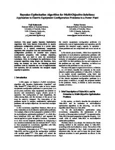
where s includes the state variables described above, and the value of is assumed to be Gaussian distributed. In this case θ has four parameters. Figure 1 shows the results for the Car Pole task. In this case MBOA can accurately model the dynamics of the system after a small number of observed trajectories. This results in fast convergence to an excellent policy which dominates the quality of the policies found by the other algorithms. Comparatively all other methods require much more data before a good policy is found. BOA always finds a policy which balances the pole for the full 1000 steps. However, some of the discovered policies have more erratic behavior decreasing the accumulated reward for each run. Q-Learning and OLPOMDP do not find comparable policies until after at least 250 additional episodes are experienced. LSPI converges faster but cannot match the performance of either the BOA or

478


Fig. 1. cart-pole Balancing Task: We report the total return per episode averaged over multiple runs of each algorithm. MBOA, BOA, and DYNA-Q are averaged over 30 runs. Q-Learning and OLPOMDP are averaged over 300 runs to control for the erratic behavior of these algorithms.

MBOA algorithm (please note our problem is distinct from the original LSPI balancing task, we allow the agent to apply less force, include boundaries for the cart, and penalize unstable policies). After 30 episodes the DYNA-Q algorithm has found a solution comparable to that of MBOA. This is not surprising given that the shaping reward provides advice useful for the local updates performed by the DYNA-Q algorithm. We have extended the model-based results by extrapolating the best solution found after convergence in order to show the comparative performance of BOA to the other direct RL methods. 4.3 3-Link Planar Arm Task In the 3-link Planar Arm task the goal is to direct an arm tip to a target region on a 2 dimensional plane. The arm is controlled by applying torques at each joint. The arm responds kinematically to the applied torques; only the torques at the joints influence the change of state. There are specified maximum joint angles, simulating the physical constraints of a real robot, preventing each joint from moving through more than 1800 of rotation. The action space in this task is three dimensional, one dimension for each joint, each of which can apply a torque of -1 or 1. The reward signal for the agent is the squared distance between the tip of the arm and the center of the target region. To handle the 3 dimensional action space a separate controller is learned for each joint. For MBOA, BOA, and OLPOMDP a logistic function controls each joint (6 total policy parameters). DYNA-Q and Q-Learning approximate separate Q-functions for each joint. The state space for each individual joint controller is simply the computed distance between the x and y coordinates of the arm tip and target locations respectively.


479

Fig. 2. Planar Arm Task: We report the total return per episode averaged over multiple runs of each algorithm. MBOA, BOA, and DYNA-Q are averaged over 30 runs. Q-Learning and OLPOMDP are averaged over 300 runs.

The relative performance of each algorithm is shown in Figure 2. Like the cart-pole task the transition and reward function can be captured by the linear model. Once the system is successfully modeled the optimization of the expected improvement quickly identifies the optimal policy. It takes several additional trials before the BOA algorithm begins finding policies of similar quality. The other model-free alternatives require 1000 episodes before converging to the same result. It is worth noting that given far more episodes the CMAC approximator for the Q-learning algorithm finds a policy superior, on average, to the BOA algorithm. The additional internal simulations clearly benefit the DYNA-Q algorithm. After 40 episodes we report the maximum average return achieved by the algorithm. DYNA-Q has found a policy comparable to the MBOA algorithm, but requires more experience. 4.4 Mountain Car Task In the mountain car domain the goal is to accelerate a car from a fixed position at the base of a hill to the hills apex. The state includes the location of the car on the hill and the car’s velocity. At each step the agent receives a reward of -1. At the end of an episode if the agent has reached the apex of the hill it receives 100 reward. To control the car the agent can apply an acceleration of -1 or 1. It is important that the accelerations are not sufficient to simply force the car up one side of the hill. Doing so would make the task too trivial. Success is only achieved by using the force of gravity to augment the cars accelerations. MBOA, BOA, and OLPOMDP optimize a logistic function to control the car (8 policy parameters). In Figure 3 we report the results for the MBOA and DYNA-Q algorithms. Due to the sparse reward signal, all of the model-free methods would appear at the base of this

480


Fig. 3. Mountain Car Task: We report the average total return per episode in the mountain car task. The MBOA and DYNA-Q results were averaged over 30 runs.

graph. We omit these uninformative results. However, the important comparison between the model-based methods shows that the MBOA algorithm makes more effective use of the continuous domain models. In this case the linear models for the system cannot fully capture the transition function for the domain. MBOA more aptly corrects for modeling errors than the DYNA-Q algorithm, which cannot ignore or correct the model when it returns erroneous results. These errors accumulate when DYNA-Q performs internal updates impacting the quality of its solution. 4.5 Acrobot Task In the acrobot domain the goal is to swing the foot of the acrobot over a specified threshold by applying torque at the hip. The state of the system includes the angle of the torso of the acrobot, the angle between the torso and legs, and the rate of change of each angle. Like the planar arm task real world constraints are placed on the articulations of the joints which prevent the legs of the acrobot from crossing through the torso. The agent can only control the behavior of the acrobot at the hip by applying a torque of -1 or 1. At each step the agent receives +100 bonus if the foot reached the goal height, or a -1 penalty in other steps. Again, MBOA, BOA and OLPOMDP optimize a logistic function governing the probability of selecting an action (6 policy parameters). This under-actuated task has a complicated transition between states. We were unable to identify even a non-linear model that predicts the controls with high accuracy. Instead the model-based systems use a linear approximation of the transition function, which when used for simulation reports incorrect returns for most of the policy space. Domains with these properties typically motivate the use of model-free methods. As indicated in Figure 4, MBOA can still make use of even this highly inaccurate model. In the initial stages of the learning process MBOA is uncertain of the quality of its


481

Fig. 4. Acrobot Task: We report the total return per episode averaged over multiple runs of each algorithm. MBOA, BOA, and DYNA-Q are averaged over 30 runs. Q-Learning and OLPOMDP are averaged over 300 runs.

model, but by modeling the residuals MBOA still benefits from the in regions where the predictions are accurate. This explains why the performance of MBOA improves over BOA’s sample complexity. Over time, as the difference in predictions increases, MBOA slowly begins ignoring the model estimates defaulting to the behavior of BOA. By contrast, because the DYNA-Q algorithm treats the model as a surrogate for the domain its estimates of the state action values are damaged during internal simulation. Regardless of the quantity of data available the assumptions made by the DYNA-Q algorithm (an assumption shared by most model-based algorithms) prevent it from learning in this context. It is worth noting that LSPI fails to improve on the performance of BOA (and barely improves on the performance of the model-free algorithms). This is additional evidence that expending some computational effort to select policies for exploration improves the quality of information observed. The reduction in exploratory episodes is considerable.

5 Conclusion We have proposed extending the Bayesian Optimization approach to RL by augmenting the surrogate function representing the expected return to have a mean which is dependent on an approximate model. The MBOA algorithm which takes advantage of the improved surrogate function is designed to both improve data efficiency when the model reasonably approximates the domain, and be robust to extreme errors in the model when it is highly inaccurate. We demonstrate the effectiveness of the MBOA algorithm in four benchmark RL domains. Empirically the MBOA algorithm outperforms LSPI, OLPOMDP, Q-Learning with CMAC function approximation, BOA, and

482


DYNA-Q in the mountain car, cart-pole, and planar arm tasks. In the case of the acrobot swing up task, where we could not find an accurate model for the domain, MBOA still outperforms all other algorithms. Empirically MBOA outperforms all of the alternatives in terms of data efficiency. This efficiency is gained at the cost of additional computation time for the simulations, which generate sample trajectories of candidate policies during optimization of the expected improvement. Overall, MBOA appears to be a useful step toward combining model-based methods with Bayesian Optimization for purposes of handling inaccurate models and improving data efficiency.

Acknowledgements We gratefully acknowledge the support of the Army Research Office under grant number W911NF-09-1-0153 and the NSF under grant number IIS-0905678.

References 1. Lizotte, D., Wang, T., Bowling, M., Schuurmans, D.: Automatic gait optimization with gaussian process regression. In: IJCAI’07: Proceedings of the 20th International Joint Conference on Artifical Intelligence, pp. 944–949. Morgan Kaufmann, San Francisco (2007) 2. Lizotte, D.: Practical Bayesian Optimization. PhD thesis, University of Alberta (2008) 3. Brochu, E., Cora, V., de Freitas, N.: A tutorial on bayesian optimization of expensive cost functions, with application to active user modeling and hierarchical reinforcement learning. Technical Report TR-2009-023 (2009) 4. Engel, Y., Mannor, S., Meir, R.: Reinforcement learning with Gaussian processes. In: International Conference on Machine Learning, pp. 201–208 (2005) 5. Dearden, R., Friedman, N., Andre, D.: Model based Bayesian exploration. In: UAI (1999) 6. Strens, M.J.A.: A Bayesian framework for reinforcement learning. In: International Conference on Machine Learning, pp. 943–950 (2000) 7. Duff, M.: Design for an optimal probe. In: International Conference on Machine Learning (2003) 8. Lagoudakis, M.G., Parr, R., Bartlett, L.: Least-squares policy iteration. Journal of Machine Learning Research 4 (2003) 9. Sutton, R., Barto, A.G.: Reinforcement Learning: An Introduction. MIT Press, Cambridge (1998) 10. Baxter, J., Bartlett, P.L., Weaver, L.: Experiments with infinite-horizon, policy-gradient estimation. Journal of Artificial Intelligence Research 15(1), 351–381 (2001) 11. Mockus, J.: Application of bayesian approach to numerical methods of global and stochastic optimization. Global Optimization 4(4), 347–365 (1994) 12. Vazquez, E., Bect, J.: Convergence properties of the expected improvement algorithm with fixed mean and covariance functions. Journal of Statistical Planning and Inference 140(11), 3088–3095 (2010) 13. Rasmussen, C.E., Williams, C.K.I.: Gaussian Processes for Machine Learning (Adaptive Computation and Machine Learning). The MIT Press, Cambridge (2005) 14. Jones, D.R., Perttunen, C.D., Stuckman, B.E.: Lipschitzian optimization without the lipschitz constant. J. Optim. Theory Appl. 79(1), 157–181 (1993)