Conceptualization of Place via Spatial Clustering and Co–occurrence Analysis Dong–Po Deng
Tyng–Ruey Chuang
Rob Lemmens
Institute of Information Science, Academia Sinica — and — International Institute for Geo–Information Science and Earth Observation (ITC)
Institute of Information Science Academia Sinica 128 Academia Road, Sec. 2 Nangang 115, Taipei Taiwan
International Institute for Geo–Information Science and Earth Observation (ITC) P.O. Box 6 7500 AA Enschede The Netherlands
[email protected]
[email protected]
[email protected]
ABSTRACT
Keywords
More and more users are contributing and sharing more and more contents on the Web via the use of content hosting sites and social media services. These user–generated contents are tagged with terms characterizing the contents from the users’ perspectives. Massive collections of tagged photos in popular photo hosting sites are well known for their richness in semantic extent and geospatial scope. Furthermore, geo–tags, which are machine–generated positional data, are frequently embedded within these photos. We develop in this paper an approach based on the analyses of tags and geo–tags for the exploration and characterization of the implicit localities in collections of user photos. At the same time, the approach also allows us to explore the meanings given by users about the places in their photo collections. In this approach, we first use DBSCAN (Density–based Spatial Clustering with Noise) to group geo–tagged photos into clusters (of possibly multiple distance scales). Then, a co– occurrence analysis on the tags used within a cluster is utilized to extract conceptualization of the place in the cluster. The extracted concepts are not necessarily of geospatial nature (e.g., airplane/airline names in photos taken in the surrounding area of an airport) so are especially useful when compared to concepts extracted via the simple use of readily available locational resources (e.g., gazetteers).
Tags, Spatial Clustering, Semantics, Data Mining, Knowledge Discovery.
Categories and Subject Descriptors H.2.8 [Database Applications]: Data Mining; H.2.8 [Database Applications]: Spatial Database and GIS; H.3.3 [ Information Search and Retrieval]: Clustering
General Terms Measurement, Experimentation, Human Factors.
Permission to make digital or hard copies of all or part of this work for personal or classroom use is granted without fee provided that copies are not made or distributed for profit or commercial advantage, and that copies bear this notice and the full citation on the first page. To copy otherwise, to republish, to post on servers or to redistribute to lists, requires prior specific permission and/or a fee. ACM LBSN ’09, November 3, 2009. Seattle, WA, USA. Copyright 2009 ACM ISBN978-1-60558-860-5 ...$10.00
1.
INTRODUCTION
It is now a common activity for people to search and share geo–referenced information and resource in the form of maps on the web such as finding locations and planning routes. The web is increasingly being seen as a platform for providing geospatial data and services. The “Web 2.0” phenomenon has further brought forward an environment of openness in which users are able to collaboratively create content and share information in their social networks. It used to be that information consumption was the norm when using the Web. In Web 2.0, however, a user often interacts with other users to create, modify, and exchange contents on the Web. The use of tagging is a noticeable practice of Web 2.0. A tagging system allows users to classify objects of interests (such as bookmarks, photos, and books) by keywords or terms. A new word, a compound of folks and taxonomy, “folksonomy” has been used to describe the practice of personal tagging of information and objects in a social environment while people consume the information and use the objects [13]. In a digital world, a large percentage of data is of geospatial nature: postal code, addresses, place names, etc. As online maps and GPS devices are frequently available, more and more digital data has been annotated with geo–tags. A geo–tag is a kind of metadata that usually consists of the latitude and longitude coordinates, though it can also include the altitude, bearing, and possibly place names. The use of the geo–tags is to identify the locations of objects, including photos, videos, web pages, and blog entries, for sharing or collaboration. Unlike geo–tags, tags are terms or keywords that are freely created by users when they would like to mark contents with meaningful descriptive terms so as to personally classify objects of their interests [5, 8]. Intuitively, as long as the user–generated contents include geo–tags, they are geospatial data. Since Web users are creating a huge volume of geo–tagged data in social networks, some interesting research questions have been raised: • Is geospatial data created in a social network a valuable
production in and for a geospatial society in general? • How to extract the geospatial information from user– generated contents in a social network? Geo–tagged (Geo–referenced) photos are one kind of geospatial data created in a social network. Meanwhile, the tags freely chosen by users to attach to these photos should give rise to emergent semantics and shared conceptualization of the places. Accumulation of tags on shared objects often can express common consensus. Users with similar interests tend to use words from a shared vocabulary. Objects of similar themes will call for a shared vocabulary as well. The act of appending tags can be considered as “voting” in which objects about a place, such as photos, are assigned meanings and their contexts. Based on the “wisdom of crowd” or collective intelligence, patterns and trends emerge from the collaboration and competition of many individuals. Based on this collective intelligence, we aim to discover how people conceptualize places. However, a set of tags is different from a category– and ontology–based system. Without priori semantics, it is a challenge to extract structured knowledge from an unstructured set of tags. It has been argued that patterns and trends emerge from the collaboration and competition of many individuals are able to turn out structured information from tag–based system despite the lack of ontology and priori defined semantics to support these tagging activities [5, 7, 9]. This paper aims to explore common consensus of places in different distance scales, as well as to discover the meanings of places that hidden in the tags that are attached to photos about the places. In summary, geo–tags in photos are machine–generated positional information about the places, and are subject to numerical and algorithmic analysis. Tags are terms that are subjective, but overlapping and correlating in their occurrences. The goal of this paper is not only to explore and experiment with separate techniques for analyzing geo–tags and tags, but also to combine the results of the analyses to gain understandings about places from user–generated contents that are marked with geo–tags and tags. Results from this research can be applied in a tag recommendation system in which tags related to a place are suggested to people who are taking photos in the area of the place. Imagine that, when you are using a GPS–equipped mobile phone to take photos in the surrounding area of Van Gogh Museum, the tag recommendation system pops up not just terms like “van”, “gogh”, and “museum” for tagging the photos, but also terms like “museumplein”, “rijksmuseum” for your choice. That is because these tags have already been found to be highly co–occurring with photos clustered by the geographic position of your GPS mobile phone. The remainder of the paper is structured as follows. We discuss related work in Section 2, which is followed by a description of how we process tagged photos from Flickr in Section 3. In Section 4 we report the usage of a spatial clustering method for classifying geo–tagged photos. In Section 5, we describe a method to discover the semantics of places in different photo clusters classified by different distance.
Finally, in Section 6 we briefly make some conclusions and explore future directions.
2.
RELATED WORK
As discussed by Gruber [6], the tag ontology is used to identify and formalize a conceptualization of tagging activities. The processing of tag ontology commits to collaborative tasks at the semantic level. He considered tagging processes in social activities lead to tag ontologies. That is, a tag ontology is possibly formed by common consensus. To further clarify it, a tag ontology, he introduced, is a conceptualization of the relationships between objects, tags, and users. As collective knowledge could be extracted from practices of folksonomy, many studies have been carried out to describe and make new proposals to better organize and expose the information collected by tagging services. In the literature, there are many statistical investigations on the structure of tag collections. Researchers, for example, derive ontology from folksonomy by identifying relationships between tags [9, 11, 14]. Besides using statistical analysis for deriving ontologies from folksonomy, other approaches have also been used. Some utilize online lexical resources like dictionaries, WordNet, Google and Wikipedia, and some use other ontologies and Semantic Web resources. There are also approaches based on ontology mapping and matching, and based on functionality that helps human actors in achieving and maintaining consensus. However, there is a lack of spatial–aware approaches to detecting the geospatial dynamics of objects (photos in our case) together with the tagging patterns on the objects.
3. DATASETS: PHOTOS AND TAGS 3.1 Flickr Photo Collection Flickr is one of the most popular photo sharing platforms. When photos are uploaded on Flickr, this service reads the EXIF metadata of the uploaded photos, including camera settings, captured time and embedded coordinates from GPS. If there is no location information in EXIF of the photos, the location information can also be annotated through their Web map service. Once the users virtually link the photos to a physical location on the map, the system assigns a set of coordinates to the photos. In general, users tend to link photos to locations in map where the photos were taken. However, different users’ perspectives would link photos to different levels of physical places. An accuracy attribute referring to the zoom level of the map is used to disclose the location of the photo, e.g., from 8 for region/city level to the most precise 16 for street level. It is known that tags being chosen to attach to photographs are related to photo subjects (events and activities), photo content (mountains and cities), time (photo taken time), components in photo (sky and cloud), and places (place names and landmark names). According to a study [14], which mapped Flickr tags onto the most common categories of WordNet, it is revealed that tag terms for locations are the most frequent (28%), followed by artifacts or objects (16%), people or groups (13%), actions or events (9%), and time (7%).
Figure 2: The top 45 most frequent tags (of the 7,564 unique tags in this study) arranged in rank order by the number of times they are tagged to photos. (a)
(b) Figure 1: The selected photos from Flickr are presented on Open Street Map (www.openstreetmap.org): (a) The overall dataset, (b) Details of the red rectangle of (a).
In this study, we collect geo–tagged photos from Flickr. The set includes photos taken between 2008–01–01 and 2008–12– 31 and geo–tagged to be in Amsterdam and the surrounding areas, shown in Figure 1. To avoid generating biased results, we filtered out some photos from our dataset by the following. Firstly, users can possibly attach the same geo–tag on a set of photos by a manual operation through Flickr. This would affect the result of a spatial cluster analysis. Thus we only selected one photo from a set of photos with the same coordinate. Second, users sometimes append the same set of tags to a series of photos. Because this would affect the co–occurrence analysis of tags, we randomly keep just one photo from the set of photos with the same set of tags. Finally, in this study we used 3,965 photos containing 36,498 tags in total. There are 7,564 unique tags.
3.2
Flickr Tag Characteristics
Figure 2 shows the distribution of the tag frequency. The x–axis is the unique tag terms, ordered by descending tag frequency. The y–axis refers to the tag frequency. In the tag frequency distribution, the farther end of the tail tags, the lower probability of occurrence. The top 5 most frequent tags in the overall area of Amsterdam are amsterdam, (the) netherlands, holland, nederland, and 2008. With respect to the task of discovering locality meaning, the tags lead-
ing in the distribution of tag frequency show administrative hierarchy of place names. However, tags of lower frequency may possibly represent more detailed information about this area. Take the tags attached to photos taken surrounding Schiphol Airport as an example. The top 5 most frequent occurring tags are schiphol, amsterdam, netherlands, airport, ams. This is an example of Flickr tags representing different information at different distance scales. This phenomena reflects the discussion of Long Tail theory [1]. The most frequently occurring 20% of items represent less than 50% of occurrences; or in other words, the least frequently occurring 80% of items are more important as a proportion of the total population. In order to discovery locality meaning from the least frequently 80% of tags, grouping photos with tags via spatial clustering would reveal more detailed conceptualization of place.
4.
SPATIAL CLUSTERING
In data mining, clustering algorithm is a useful method to group data sets into meaningful classes (i.e., clusters) so that it minimizes the intra–differences and maximizes the inter– differences of the subclasses [12]. In a geo–referenced space, the most obvious measure of similarity is Euclidean distance, although other derived distances are possible. Thus, similarity measurement between geo–referenced entities is relatively well defined [2]. Moreover, there are three advantages of spatial clustering approaches for knowledge extraction: (1) minimal requirements of domain knowledge to determine the input parameters; (2) discovery of clusters with arbitrary shape; and (3) good efficiency on large databases [10]. Clusters of geo–tagged photos by Euclidean distance often represent hot spots of users’ interests in the geographic space. However, granularity of place is able to influence clustering results. The larger the extent of a place, the longer the distance the activities occur in. Therefore, for conceptualization of place, it is necessary to navigate the clusters at different distance scales.
4.1
DBSCAN (Density–Based Spatial Clustering with Noise)
DBSCAN, presented by Ester et. al. [2], is a density–based clustering method initially developed to cluster point objects. The associated algorithm requires two input parameters: EPS (given radius) and MinPts (minimum number of objects). The neighborhood of a given point p is examined
and judged to be sufficiently dense if the number of data points within a distance g from p is greater than MinPts. If so, p is called a core point and forms an initial cluster for the data set. The neighborhood within radius g from the point p is called the g–neighborhood of p. All point objects of the data set that lie within the EPS –neighborhood of p are called non–core points of the initial cluster of p. An overview of the major notions related to DBSCAN algorithm is as follows [2]. Definition 1. (directly density–reachable) An object p is directly density–reachable from an object g with respect to EPS and MinPts in the set of objects D if (1) p ∈ N EPS (q) (N EPS (q) is the subset of D contained in the EPS –neighborhood of q); (2) Card(N EPS (q)) ≥ MinPts, where Card(·) means the number of objects in a set. Definition 2. (core object and border object) An object is a core object if it satisfies Condition 2 of Definition 1. A border object is such an object that is not a core one itself but directly density–reachable from another core object. Definition 3. (density–reachable) An object p is density– reachable from an object q w.r.t. EPS and MinPts in the set of objects D, denoted as p > Dq , if there exists a chain of objects p1 , . . . , pn , p1 = q, pn = p such that pi ∈ D and pi+1 is directly density–reachable from pi w.r.t. EPS and MinPts.
Figure 3: Number of clusters and percentage of unclustered photos at different radius scales. (2) Given a cluster C and an arbitrary core object p ∈ C, C equal the set {o|o > Dp }. To find a cluster, DBSCAN starts with an arbitrary object p in D and retrieves all objects of D density–reachable from p with respect to EPS and MinPts. If p is a border object, no objects are density–reachable from p and p is assigned to noise temporarily. The clustering formed from DBSCAN follows the steps below [12]:
Step 1: Give the parameter values for EPS and MinPts. Definition 4. (density–connected) An object p is density– connected to an object q with respect to EPS and MinPts in the set of objects D if there exists an object o ∈ D such that both p and q are density–reachable from o w.r.t. EPS and MinPts in D. Definition 5. (cluster) A cluster C w.r.t. EPS and MinPts in D is a non–empty subset of D satisfying the following conditions: (1) maximality: ∀p, q ∈ D, if p ∈ C and q > Dp with respect to EPS and MinPts, then also q ∈ C; (2) connectivity: ∀p, q ∈ C, p is density–connected to q with respect to EPS and MinPts in D. Definition 6. (noise) Let C 1 , ..., C k be the clusters with respect to EPS and MinPts in D, then we define the noise as the set of objects in D not belonging to any cluster Ci , i.e. noise = {p ∈ D | ∀i : p ∈ / C i }. The procedure for finding a cluster is based on the fact that a cluster can be determined uniquely by any of its core objects: (1) Given an arbitrary object p for which the core object condition holds, the set {o|o > Dp } of all objects o density–reachable from p in D forms a complete cluster C and p ∈ C;
Step 2: Form the initial clusters by applying the following rule: For each point p of the data set, examine if it is a core point. If so, generate a new cluster with core point for point p and non–core points all other points of the set that lie within the g–neighborhood of p. Step 3: Compare repeatedly the initial clusters in pairs. If the core point in one cluster is a non–core point in the other cluster, merge the two clusters into one. Step 4: If a point is assigned as a non–core point to more than one cluster, remove it so that it is assigned to only one of them. At the end of this process, each data point is assigned to one or no clusters. In the latter case, the point is considered to be noise.
4.2
Spatial Clustering of Geo–tagged Photos
In this study clusters of geo–tagged photos are generated by the statistical computing software R. We use an R package named “fpc” (fixed point clusters, cluster–wise regression, and discriminant plots) including DBSCAN clustering by Fraley and Raftery [4]. To generate clusters at different distance scales, we fix the parameter MinPts (the minimum number of the photos) to 8 photos, and use EPS (the given radius) from 5,000 meters to 15 meters. The results basically show that the number of clusters increases as the radius decreases. When the radius is less than 2,500 meters, clusters are formed and distinguished. When
the radius is 75 meters, the number of clusters increases to the maximum. Meanwhile, the number of unclustered photos also increases as the radius decreases. If the radius parameter is too small, the result of spatial clustering would possibly lose much information (most of the photos unclustered). Similarly, if the radius parameter is too large, the result is not informative either as most photos fall into a few clusters. Figure 3 shows the number of clusters, as well as the percentage of unclustered photos, as a function of the radius size. It shows that at about 75 meters we have the most number of clusters (while the percentage of unclustered photos increases to 63%). For even smaller radiuses, the clustering effect shows deterioration. Figure 4 show the formation of clusters for radius of sizes from 2,500 meters to 75 meters on two–dimensional planes in which the dots are photos, same–colored dots are in the same cluster, and black dots are unclustered photos.
(a) 75 meters
(b) 100 meters
(c) 150 meters
(d) 200meters
(e) 250 meters
(f) 500 meters
(g) 1000 meters
(h) 1500 meters
(i) 2000 meters
(j) 2500 meters
5. CO–OCCURRENCE ANALYSIS OF TAGS 5.1 Tag–Photo Matrix The idea of photo–tag matrix comes from document–term matrix that is used in natural language processing. Document– term matrix is a processing technique to transform a natural language document to a mathematical object (a matrix), making it possible to do statistical analysis. Like document– term matrix, tag–photo matrix is a large matrix representing every photo and tag in each clusters that are generated from DBSCAN clustering. For clarity here is an example explaining the tag–photo matrix. In this example there are seven photos including 14 tags and 4 unique tags as following: Photo 1 (Tag1, Tag3, Tag4) Photo 2 (Tag1, Tag4) Photo 3 (Tag1, Tag3) Photo 4 (Tag2) Photo 5 (Tag1, Tag2, Tag3) Photo 6 (Tag1, Tag4) Photo 7 (Tag3) We can fill in the tag–photo matrix by going through every tag set of the photos and marking the cells for all the tags that appear in it, as shown in Table 1. The cell ai,j of this matrix contain occurrence tag ti in photos pj . In the other, the rows of the matrix correspond to tags, and the columns correspond to photos. We generate tag–photo matrix for each cluster via a text mining package (tm) in R developed by Feinerer et. al. [3]. If a document contains both the terms Tag1 and Tag2, these two terms are said to co–occur, or to have a first order co– occurrence. Now assume that the terms Tag1 and Tag3 co–occur in some document a, and that Tag2 and Tag3 co– occur in another document b. The terms Tag1 and Tag2 are then said to have a second order co–occurrence via the word Tag3. Based on the co–occurrence of tags, we can detect the relationships of these tags. Most people select terms to attach to photo by their perspectives of the photos.
Figure 4: Formation of clusters at different radius scales.
Table 1: An example of tag–photo matrix. Tag1 Tag2 Tag3 Tag4
P1 1 0 1 1
P2 1 0 0 1
P3 1 0 1 0
P4 0 1 0 0
P5 1 1 1 0
P6 1 0 0 1
P7 0 0 1 0
Table 2: A tag–tag correlation matrix. Tag1 Tag2 Tag3 Tag4
Tag1 1.000 -0.300 -0.091 0.730
Tag2 -0.300 1.000 -0.548 -0.091
Tag3 -0.091 -0.548 1.000 -0.417
Tag4 0.730 -0.091 -0.417 1.000
Although tags in the same cluster will contain many common tags, there are still idiomatic tags in the cluster. Some tags only occur in very few photos, and the tag–photo matrix of a cluster is often very sparse. Fortunately the text mining (tm) package of R provides methods to remove sparse terms [3]. Generally speaking, reducing sparse terms would not lose significant relations inherent in a tag–photo matrix.
5.2
Co–occurrence Correlation Analysis
Based on the tag–photo matrix, we can easily observe the presence or absence of every tag in a photo. A common approach for measuring relatedness between the tags is to compute their correlation coefficient. Pearson’s correlation coefficient takes into consideration similarity in occurrences. Take Table 1 as an example, we can calculate the tag–tag correlation matrix from the tag–photo matrix, as shown in Table 2. Tag1 and Tag4 has the highest co–occurrence in Table 1, so that the highest correlation coefficient occurs in between Tag1 and Tag4. We calculate the tag–tag correlation matrix for every cluster. Since the clusters are determined at different distance scales, the co–occurrences between tags at different distance scales can also be observed. Thus we can observe the correlation between the tag “amsterdam” and tags referring to landmarks in Amsterdam such as “schiphol”, “anne frank”, “artis”, “rijksmuseum”, “dam”, “stations”, “centraal”, “rembrandt”, and “rembrandtplein”. Figure 5 displays the tendency of tag correlation at different distance scales. Those tags have high correlationships to the tag “amsterdam” when the distance scale is less than 150 meters. Besides the tag “schiphol”, the tags associated to the landmarks of Amsterdam have highest correlationships to the tag “amsterdam” at distance scale of 75 meters. It means that clustering with a 75–meters distance is an effective way to detect tag relationships in the downtown area of Amsterdam. The Schiphol airport is larger than other landmarks, so that the highest correlation occurs in stead at the 100–meters distance scale.
5.3
Visualization of Tag Co–occurrence
Based on the co–occurrence relationships of tags, we can link tags together so as to explicitly represent possible conceptualizations of a place. It is easy to realize that Figure 6(a) is representing Rijksmuseum. Because Van Gogh Museum is close to Rijksmuseum, most people also visit Van Gogh
Figure 5: The correlation between the tag “amsterdam” and the tags of several landmarks associated to Amsterdam.
Museum after going to Rijksmuseum. That is why the relationship between the tag “rijksmuseum” and the tag “museum” is highest in this area. Museumplein is located in between Rijksmuseum and Van Gogh Museum. There is a large logo “I amsterdam” in this plaza. This logo easily attracts people to take photo when people are going though this plaza. The tag “rijksmuseum”, “van”, “gogh”, “museum”, “museumplein” and “iamsterdam” present the elements in this area. The other tags, such as “amsterdam”, “netherlands”, “holland”, and “europe” are some implicit geospatial conceptions of this area. The well–known geospatial conception is that Amsterdam is located in the Netherlands and the Netherlands is located in the Europe. For tourism, it is a intuitive way to choose these tags to identify their photos. Note that in Figure 6, the links connecting two tags are also distinguished by their width. The thicker the lines, the stronger the correlation. Similarly, tag co–occurrences in Figure 6(b) clearly presents the landmark Anne Frank House. The Jordaan area is a neighborhood of Amsterdam; it includes Canal Prinsengracht, Church Westerkerk, and Anne Frank House. It is reasonable that people who walk along with Canal Prinsengracht will also visit Church Westerkerk and Anne Frank House. Let us move outside of downtown Amsterdam. Figure 6(c) presents Airport Schiphol. Besides place name, the tags appearing in Figure 6 are elements of an airport. The tag “klm” stands for Royal Dutch Airlines. The tag “boeing” is used to describe the type of airplane, for example Boeing 747, so that the tag “boeing” has higher correlation with tag “aircraft” than with other tags.
5.4
Conceptualizing Place at Different Scales
We summarize the observations on the conceptualization of Amsterdam as informed by clusters at different radius scales. When the radius is 2,500 meter, two clusters of the photos are formed. One cluster is about an area surrounding the runways in the northwest side of Schiphol Airport. Intuitively, these photos are taken by people observing airplanes in this area. The tags on these photos are related to airplanes. The other is a large cluster covering the entire downtown Amsterdam. However, this cluster displays only city–scale conceptualization, but not landmark–scale con-
ceptualization. This is illustrated in Figure 7 where downtown Amsterdam is conceptualized via tag co–occurrence at different radius scales. At 2,500 meters, the conceptualization show tags “europe”, “netherlands”, “north”, “nederland”, “noorholland”, and “amsterdam”, which are large administrative areas associated to Amsterdam. The tags “canal” and “architecture” also appear. They represent people’s general impression about Amsterdam. When the radius is reduced to 2,000 meters, the cluster of Schiphol Airport is formed. The co–occurring tags are “schiphol”, “terminal”, “airplanes”, “klm”, etc. which show the characteristics of an airport. The conceptualization of the Schiphol Airport is quite stable: Even as the radius decreases, this place is conceptualized by almost the same set of tags. When the radius is 1,500 meters, the concepts of the satellite towns are formed, e.g., Halfweg and Amstelveen. As the radius goes down to 1,000 meters, we find clusters distinguished by parks surrounding downtown Amsterdam. At the 500–meters scale, a cluster forms at southern downtown Amsterdam. That is Buitenveldert which is a district designed by the idea of a garden city. The landmarks in downtown Amsterdam are gradually distinguished at 200– to 75–meters radiuses. Both the 200– and 150–meter scaled clusters of downtown Amsterdam include several landmarks: Anne Frank House, Rijksmuseum, Dam Square, Centraal Station, Rembrandt Museum, and the red light district. Decreasing the radius further to 100 meters, we still find Dam Square, Centraal Station, and the red light district in the same cluster. When the radius is 75 meters, the conceptualization of red light district is distinguished. Figure 7 shows the gradual formation of locality as the radius decreases. In summary, small–scale landmarks rarely form concepts in large–radius clusters of tags. To identify various conceptualization of places within a city, it is necessary to consider tag co–occurrences in small–radius clusters.
6.
CONCLUSION AND FUTURE WORK
In this study we describe an approach to the conceptualization of places via measuring co–occurrence of tags in spatial clusters at different distance scales. We have presented an implementation and the results of our experiments. The results show that a conceptualization of place is unveiled by tag co–occurrences at a suitable distance scale. If the spatial extent of the place is small (e.g., city landmark), tags pertaining to the place co–occur evidently in photos clustered by a small distance (75 meters). Furthermore, without the use of suitable spatial clustering, detailed information about a place is veiled by high frequency tags. Based on this result, location–based applications can be developed to suggest tags to users as they take photos. Although we can discover the intensity of tag co–occurrence in a cluster, this approach, however, cannot detect semantic relationships between pairs of tags. In the future we will ground the semantics between pairs of tags via the use of gazetteers or dictionaries. We expect this will help us identify the relationship types between concept pairs as depicted in Figures 6 and 7, and to extract more information from collaborative geospatial data in social environments.
7.
REFERENCES
[1] C. Anderson. The long tail. Wired, 12.10, 2004.
[2] M. Ester, H.-P. Kriegel, J. Sander, and X. Xu. A density–based algorithm for discovering clusters in large spatial databases with noise. In Proceedings of International Conference on Knowledge Discover and Data Mining, pages 226–231, 1996. [3] I. Feinerer, K. Hornik, and D. Meyer. Text mining infrastructure in R. Journal of Statistical Software, 25(5):1–54, February 2008. [4] C. Fraley and A. E. Raftery. Model–based clustering, discriminant analysis, and density estimation. Journal of the American Statistical Association, 97:611–631, 2002. [5] S. A. Golder and B. A. Huberman. Usage patterns of collaborative tagging systems. J. Inf. Sci., 32(2):198–208, 2006. [6] T. Gruber. Ontology of folksonomy: A mash-up of apples and oranges. International Journal on Semantic Web and Information Systems, 3:1–11, 2007. [7] C. Marlow, M. Naaman, D. Boyd, and M. Davis. Ht06, tagging paper, taxonomy, Flickr, academic article, to read. In HYPERTEXT ’06: Proceedings of the seventeenth conference on Hypertext and hypermedia, pages 31–40, New York, NY, USA, 2006. ACM. [8] T. Rattenbury, N. Good, and M. Naaman. Towards automatic extraction of event and place semantics from Flickr tags. In SIGIR ’07: Proceedings of the 30th annual international ACM SIGIR conference on Research and development in information retrieval, pages 103–110, New York, NY, USA, 2007. ACM. [9] T. Rattenbury and M. Naaman. Methods for extracting place semantics from Flickr tags. ACM Trans. Web, 3(1):1–30, 2009. [10] J. Sander, M. Ester, H.-P. Kriegel, and X. Xu. Density–based clustering in spatial databases: The algorithm GDBSCAN and its applications. Data Min. Knowl. Discov., 2(2):169–194, 1998. [11] P. Schmitz. Inducing ontology from Flickr tags. In Workshop on Collaborative Web Tagging at WWW2006, 2006. [12] E. Stefanakis. Net–dbscan: clustering the nodes of a dynamic linear network. International Journal of Geographical Information Science, 21(4):427–442, 2007. [13] T. Vander Wal. Folksonomy. http://www.vanderwal.net/folksonomy.html, 2007. [14] X. Wu, L. Zhang, and Y. Yu. Exploring social annotations for the semantic web. In WWW ’06: Proceedings of the 15th international conference on World Wide Web, pages 417–426, New York, NY, USA, 2006. ACM.
rijksmuseum
north
van
noordholland
netherlands netherlands
nederland
museum
nederland
holland
museumplein
holland europe
europe
iamsterdam
canal
gogh
architecture
amsterdam amsterdam
(a) Rijksmuseum
(a) Downtown Amsterdam cluster at 2,500 meters.
the
westerkerk
van
station
prinsengracht
red
netherlands netherlands
jordaan
holland
nederland
light
holland
church
frank
jordaan
dam
anne
canal
canal boat
bike
amsterdam
amsterdam
(b) Anne Frank House
(b) Downtown Amsterdam cluster at 150 meters.
schipol
sex
street
red
schiphol
netherlands
netherlands
nederland light
amsterdam
holland
klm
holland
district
ams
blue canal
airport amsterdam
(c) Red light district cluster at 75 meters
aircraft
(c) Schiphol Airport Figure 6: Tag co–occurrences in the 75–meters scaled clusters. The thicker a line, the higher the correlation between the pair of tags it connects.
Figure 7: Tag co–occurrences at differently scaled clusters. The thicker a line, the higher the correlation between the pair of tags it connects.