Speech Utterance Clustering Based on the Maximization of Within-cluster Homogeneity of Speaker Voice Characteristics Wei-Ho Tsai1 and Hsin-Min Wang2 1
Department of Electronic Engineering, National Taipei University of Technology, Taipei, Taiwan E-mail:
[email protected], Phone: +886-2-27712171 ext. 2257, Fax: +886-2-27317120 2
Institute of Information Science, Academia Sinica, Taipei, Taiwan
E-mail:
[email protected], Phone: +886-2-27883799 ext. 1714, Fax: +886-2-27824814
Abstract This paper investigates the problem of how to partition unknown speech utterances into a set of clusters, such that each cluster consists of utterances from only one speaker, and the number of clusters reflects the unknown speaker population size. The proposed method begins by specifying a certain number of clusters, corresponding to one of the possible speaker population sizes, and then maximizes the level of overall within-cluster homogeneity of the speakers’ voice characteristics. The within-cluster homogeneity is characterized by the likelihood probability that a cluster model, trained using all the utterances within a cluster, matches each of the within-cluster utterances. To attain the maximal sum of likelihood probabilities for all utterances, the proposed method applies a genetic algorithm to determine the cluster in which each utterance should be located. For greater computational efficiency, also proposed is a clustering criterion that approximates the likelihood probability with a divergence-based model similarity between a cluster and each of the withincluster utterances. The clustering method then examines various legitimate numbers of clusters by adapting the Bayesian information criterion to determine the most likely speaker population size. The experimental results show the superiority of the proposed method over conventional methods based on hierarchical clustering. PACS numbers: 43.72.Pf [DDO] Running title: Speaker Clustering 1
I. INTRODUCTION For more than two decades, automatic speaker recognition based on vocal characteristics [5][35][38] has received a tremendous amount of attention in research that facilitates human-machine communications and biometric applications. Nowadays, as speech is being exploited as an information source, the utility of recognizing speakers’ voices is increasingly in demand for indexing and archiving the mushrooming amount of spoken data available universally. Traditional approaches to speaker recognition assume that some prior information or speech data is available about the speakers concerned. Thus, speaker-specific models can be trained using the labeled speech data, and the likelihoods of unknown test utterances can then be computed from the models, thereby determining the identity of a speaker (speaker identification), or determining if a speaker is who he/she claims to be (speaker verification). However, for indexing or archiving, the basic strategy needs to be expanded to distinguish between speakers when neither information about the speakers’ voices nor the speaker population size is available. As a result, unsupervised classification of speech data based on speakers’ voice characteristics has emerged as a new and challenging research problem [23][24][29][44][47]; however, the solutions to this problem require further investigation. Classifying speech data by speaker is generally associated with two processes. One is to segment speech data into homogenous utterances that contain only one speaker’s voice. The other is to group together homogeneous utterances from the same speaker into a cluster. The former is usually referred to as speaker segmentation [18][47], while the latter is referred to as speaker clustering [40][44]. A joint process consisting of speaker segmentation and clustering, called speaker diarization [3][31][34][45] was recently defined by the NIST Speech Group [33]. It is hoped that by locating speech segments from the same speaker, the human effort required for indexing speech data can be greatly reduced from having to listen to every long audio recording to only having to check a few utterances in each cluster. In addition, by locating speech utterances from speakers with similar voices [9][12][21], transcription or recognition of speech messages can be carried out more effectively by adapting acoustic models on a per cluster basis, which exploits more adaptation
2
data than on a per utterance basis. In this paper, we concentrate on the problem of speaker clustering. Given N unlabeled speech utterances, each of which is assumed to be from one of P speakers, where N ≥ P and P is unknown, speaker clustering is defined as the partitioning of N utterances into M clusters, such that M = P , where each cluster consists exclusively of utterances from only one speaker. For utterances that contain multiple speakers, the partitioning is preferably performed after the utterances are pre-segmented into speaker-homogeneous regions. However, in order to focus on the fundamental techniques for speaker clustering, this study does not investigate the speaker-segmentation problem, but only deals with utterances containing a single speaker. Currently, most speaker-clustering methods follow a hierarchical clustering framework [6][8][12] [17][27][28][32][40][42][44], which consists of three major components: computation of inter-utterance similarities, generation of a cluster tree, and determination of the number of clusters. Similarity computation is designed to produce larger values for similarities between utterances of the same speaker and smaller values for similarities between utterances of different speakers. Several similarity measures, such as the Arithmetic Harmonic Sphericity (AHS) [18], Kullback Leibler (KL) distance [42], the Cross Likelihood Ratio (CLR) [40], and the Generalized Likelihood Ratio (GLR) [12][27][44], have been examined and compared in much of the literature, with GLR being the most prevalent similarity measure. The generation of a cluster tree can be performed in either a bottom-up (agglomerative) or a top-down (divisive) fashion, according to some criteria drawn from the similarity measure. The bottom-up approach starts with each utterance as a single cluster, and then successively merges the most similar pairs of clusters until one cluster contains all the utterances. The similarities between clusters are usually derived from the inter-utterance similarities, based on so-called complete linkage, single linkage, or average linkage. In the top-down approach, all utterances start in a single cluster, which is split into two dissimilar clusters. This procedure is then repeated for each of the dissimilar clusters, until each cluster contains exactly one utterance. The resulting cluster tree is then cut via an estimation of the number of clusters to retain the best partitioning. Representative methods for estimating the optimal number of 3
clusters are based on the BBN Metric [44] and the Bayesian Information Criterion [6]. In essence, the effectiveness of a speaker clustering system depends on whether or not the generated clusters are related to speakers, rather than other acoustic classes. In the hierarchical clustering framework, inter-utterance similarity computation plays a crucial role in determining if the clusters are formed on the basis of speakers. However, existing similarity measures, based on AHS, KL distance, CLR, or GLR, are performed entirely on spectrum-based features, such as Mel-scale Frequency Cepstral Coefficients (MFCCs) and Perceptual Linear Prediction (PLP) cepstral coefficients. These features are known to carry various types of information besides a speaker’s voice characteristics, for example, phonetic and environmental information. Although feature normalization techniques, such as cepstral mean subtraction [10] and RASTA [14], may be applied to alleviate the interference from the channels and noise, these techniques also run the risk of removing the target speakers’ voice characteristics, especially when the utterances are short. As a result, there is no guarantee that the similarities between same-speaker utterances will always be larger than the similarities between different-speaker utterances. Since inter-utterance similarity computation is independent of cluster tree generation, and the latter trusts the former completely, the inevitable errors of inter-utterance similarity can propagate down the whole process, which severely limits the clustering performance. To compensate for the imperfection of inter-utterance similarity computation, more sophisticated speaker-clustering methods [3][44] have tried to improve the measurement of inter-cluster similarities by concatenating all the utterances within each cluster into one long utterance and then computing the similarities between long utterances. Analogously, recent speaker-diarization systems, such as [43] and [48], further apply modeling and matching techniques in speaker identification to evaluate inter-cluster similarities. Specifically, each cluster is represented as a Gaussian mixture model (GMM) by using the so-called GMM-UBM method [38]. Then, the similarity between a pair of clusters is computed by accumulating the likelihoods of one cluster’s utterances testing against another cluster’s model. On the other hand, in the context of acoustic model adaptation for speech recognition, [19] proposes using an MLLR-adapted likelihood as a criterion, 4
instead of the inter-cluster similarity measurement, to determine which speech data should be grouped together and handled by the same MLLR transforms, such that the mismatch between speech-recognition models and test data can be minimized. In addition, [19] and the subsequent Cambridge speaker-diarization systems [43] use gender and bandwidth classification to pre-process speech utterances, which allows data from different-gender speakers or different types of channel to be processed separately, thereby reducing the confusion as well as the load on clustering. Meanwhile, in [48], a feature warping technique [36] is used to further reduce the effects of the acoustic environment. However, one unresolved problem in most existing systems is the propagation of errors in hierarchical clustering. Taking agglomerative clustering as an example, during the merging process, the utterances from different speakers may be mis-grouped into a cluster. Since the mis-grouped utterances will never be separated in the subsequent merging operations, such errors will proliferate as more clusters are merged. On the other hand, cluster tree generation based on either top-down or bottom-up hierarchical clustering usually uses a certain neighborhood selection rule, e.g., nearest or furthest neighbor, to determine which utterances should be assigned to which clusters. However, the neighborhood selection rule is applied in a cluster-by-cluster or pairwise manner, rather than in a global manner that considers all the clusters simultaneously. As a consequence, hierarchical clustering can only make each individual cluster as homogeneous as possible, but cannot attain the ultimate goal of maximizing the overall homogeneity. To overcome the limitations of the hierarchical speaker-clustering framework, this study proposes a new clustering method, with the goal of finding the best partitioning of speech utterances by integrating inter-utterance similarity computation and cluster tree generation into a unified process. The process iteratively assigns speech utterances to a set of clusters and creates a stochastic model for each cluster, which attempts to maximize the similarity or agreement between each cluster model and the within-cluster utterances. In contrast to a similar idea proposed in [19], which uses a top-down split-and-merge framework to achieve the goal of the maximum likelihood of adapted data, we apply a genetic algorithm [13], together with a model similarity comparison 5
method, to search for the best partitioning. In addition, the proposed clustering method further adapts the Bayesian information criterion to determine how many clusters should be created. The remainder of this paper is organized as follows. Section II reviews a specific implementation of hierarchical clustering, which is the most popular method of speaker clustering. Section III introduces our proposed speaker clustering method, called maximum likelihood clustering, with the goal of maximizing the within-cluster homogeneity of voice characteristics. In Section IV, we present an alternative speaker-clustering solution, called minimum divergence clustering, which aims to improve the efficiency of maximum likelihood clustering. Section V discusses the problem of how to automatically determine the appropriate number of clusters. Section VI summarizes the configuration of our speaker-clustering system, and analyzes its computational complexity. Section VII presents our experimental results. Finally, in Section VIII, we present our conclusions, and discuss the direction of future works.
II. REVIEW OF HIERARCHICAL CLUSTERING To cluster speech utterances by speaker, it is necessary to distinguish between utterances belonging to the same speaker and those belonging to different speakers. A common strategy for this process is to measure the similarities of voice characteristics between utterances, and then determine which utterances are similar enough to be considered as being from the same speaker. This section details a specific implementation of this strategy, which serves as a baseline solution in the current study. A. Inter-utterance Similarity Computation Let X1 , X2 , . . . , XN denote N speech utterances to be clustered, each of which is represented by a certain spectrum-based feature, e.g., the cepstral feature. The similarities between utterances are measured on the basis of the Generalized Likelihood Ratio (GLR) [12]. For any pair of utterances, Xn and Xk , GLR is computed by GLR(Xn , Xk ) =
Pr(Xn |λnk ) Pr(Xk |λnk ) , Pr(Xn |λn ) Pr(Xk |λk )
(1) 6
or, equivalently, GLR(Xn , Xk ) = log Pr(Xn |λnk ) + log Pr(Xk |λnk ) − log Pr(Xn |λn ) − log Pr(Xk |λk ),
(2)
where λn , λk , and λnk are stochastic models, e.g., Gaussian mixture models (GMMs), trained using Xn , Xk and a concatenation of Xn and Xk , respectively. These stochastic models are designed to capture the relevant aspects of voice characteristics underlying speech utterances. Implicit in Eq. (1) and (2) is the presumption that if utterances Xn and Xk are from the same speaker, model λnk should be able to cover the voice characteristics of the individual utterances appropriately; hence, the likelihood probabilities Pr(Xn |λnk ) and Pr(Xk |λnk ) would be large, compared to the case where utterances Xn and Xk are from different speakers. This gives a large value of GLR(Xn , Xk ) when utterances Xn and Xk are from the same speaker, and a small value otherwise. B. Cluster Generation After computing the inter-utterance similarities, the next step is to assign the utterances deemed similar to each other to the same cluster. This is commonly done by an agglomerative hierarchical clustering method [20], which consists of the following procedure: 1. 2. 3. 4. 5. 6. 7.
begin initialize M ← N , and form clusters ci ← {Xi }, i = 1, 2, · · · , N do find the most similar pair of clusters, say ci and cj merge ci and cj M ←M −1 until M = 1 end The similarities between a pair of clusters, say ci and cj , can be derived from the inter-utterance
similarities, according to one of the following heuristic measures: 1) Complete-linkage S(ci , cj ) =
min
GLR(Xn , Xk );
(3)
max
GLR(Xn , Xk ); or
(4)
Xn ∈ci ,Xk ∈cj
2) Single-linkage S(ci , cj ) =
Xn ∈ci ,Xk ∈cj
7
3) Average-linkage S(ci , cj ) =
X 1 GLR(Xn , Xk ), #(i, j) Xn ∈ci ,Xk ∈cj
(5)
where #(i, j) denotes the number of utterance pairs involved in the summation. Alternatively, the similarities between clusters can be measured by concatenating all the utterances within each cluster into a long utterance, and then computing the GLR between the concatenated utterances. The outcome of the agglomeration procedure is a cluster tree. The final partition of the utterances is then determined by pruning the tree that only has the desired number of leaves left.
III. MAXIMUM LIKELIHOOD CLUSTERING (MLC) Although the above hierarchical-clustering method is popular for speaker clustering, it is far from optimal in a number of respects. First, the similarities between utterances are measured in a pairwise manner, which only considers information about one pair of utterances at a time, and ignores the fact that out-of-pair information can benefit similarity computation for every pair of utterances. Obviously, a better solution would be to characterize the similarities between all the utterances to be clustered in a global fashion, rather than in a piecemeal manner. Second, hierarchical clustering only attempts to make the voice characteristics within a newly generated cluster as homogenous as possible. However, it cannot guarantee that the homogeneity for all the clusters can be summed to reach a maximum, since its decision does not consider the interaction between the new cluster to be generated and existing clusters. Consequently, some mis-clustering errors, arising from grouping different-speaker utterances together, can propagate down the whole process and hence limit the clustering performance. To overcome these shortcomings, we present a new clustering method based on the integration of similarity computation and cluster generation, which aims to maximize overall within-cluster homogeneity. A. Principle
8
Recall that in GLR-based similarity measurement, it is assumed that the voice characteristics of a pair of utterances can be well represented by using a single model instead of two utteranceindividual models, if both utterances are from the same speaker. Likewise, if several utterances are from the same speaker, they can be pooled to form a joint model without distorting their individual voice characteristics. In other words, if a model trained using a group of utterances is capable of characterizing the utterances consistently well, then these utterances are very likely produced by the same speaker. Therefore, we can formulate speaker clustering as a problem of determining which utterances should be grouped together such that the resultant models can best characterize the grouped utterances. The proposed method begins by specifying a certain number of clusters to be generated. For any given number of clusters, M , the task of speaker clustering is to assign N utterances X1 , X2 , . . . , XN to M clusters c1 , c2 , . . . , cM . Let gn denote the index of the cluster that an utterance, Xn , is assigned to, where gn is an integer between 1 and M . The goal of optimal clustering ∗ is, therefore, to produce a set of cluster indices, G∗ = {g1∗ , g2∗ , . . . , gN }, satisfying gn∗ = gk∗ for
any utterances Xn and Xk from the same speaker, and gn∗ 6= gk∗ for utterances Xn and Xk from different speakers. Toward this end, we first create a Gaussian mixture model λ(m) for each cluster cm , 1 ≤ m ≤ M , by using all the feature vectors of the utterances assigned to cm . Then, a certain level of agreement that the utterances assigned to the same cluster come from the same speaker is characterized by computing the likelihood probability Pr(Xn |λ(m) ) for every gn = m. Conceivably, the larger the value of Pr(Xn |λ(m) ), the more suitable cluster cm will be for utterance Xn . Thus, by taking the likelihood probabilities for all the utterances into account, G∗ can be determined by G∗ = arg max G
M X N X
log Pr(Xn |λ(m) )δ(gn , m),
(6)
m=1 n=1
where δ(·) is a Kronecker Delta function. We refer to this process as maximum likelihood clustering (MLC). As Eq. (6) is equivalent to G
∗
= arg max G
M X N h X
i
log Pr(Xn |λ(m) ) − log Pr(Xn |λn ) δ(gn , m),
m=1 n=1
9
(7)
in which the term log Pr(Xn |λn ) is a constant that is independent of clustering, MLC can be viewed as the maximization of the overall within-cluster GLRs, given a certain number of clusters. B. Optimization via the Genetic Algorithm Although the solution to Eq. (6) exists, no close form can be derived from this equation directly. Moreover, since the cluster indices are not scalar objects, we cannot use a gradient-based optimization in this scenario. It is also infeasible to perform an exhaustive search, which examines all possible solutions to determine the best one, because there are M N possible combinations of cluster indices, and this task is an NP-complete problem. Recognizing these difficulties, we propose applying the genetic algorithm (GA) [13] to find G∗ by virtue of its global scope and parallel searching power. The basic operation of the GA is to explore a given search space in parallel by means of iterative modification of a population of chromosomes. Each chromosome, encoded as a string of alphabets or real numbers called genes, represents a potential solution to a given problem. In our task, a chromosome is exactly a legitimate G, and a gene corresponds to a cluster index associated with an utterance. However, since the index of one cluster can be interchanged with that of another cluster, multiple chromosomes may reflect an identical clustering result. For example, the chromosomes {1, 1, 1, 2, 2, 3, 3}, {1, 1, 1, 3, 3, 2, 2}, {2, 2, 2, 1, 1, 3, 3}, {2, 2, 2, 3, 3, 1, 1}, {3, 3, 3, 2, 2, 1, 1}, and {3, 3, 3, 1, 1, 2, 2} represent the same clustering result of grouping seven utterances into three clusters. Such a non-unique representation of the solution would significantly increase the GA search space, and could lead to an inferior clustering result. To avoid this problem, we limit the inventory of chromosomes to conform to a baseform representation defined as follows. Let I(cm ) be the lowest index of the utterance in the m-th cluster, cm = {Xi |gi = m, 1 ≤ i ≤ N }. A chromosome is a baseform iff ∀ cm and cl , if m < l, then I(cm ) < I(cl ).
(8)
As the above example shows, chromosome {1, 1, 1, 2, 2, 3, 3} is a baseform, since the lowest indices of the utterances in the first, second, and third clusters are 1, 4, and 6, respectively, which 10
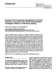
satisfies Eq. (8). In contrast, chromosome {1, 1, 1, 3, 3, 2, 2} is not a baseform, since the lowest indices of the utterances in the first, second, and third clusters are 1, 6, and 4, respectively, which does not satisfy Eq. (8). Likewise, the other chromosomes, {2, 2, 2, 1, 1, 3, 3}, {2, 2, 2, 3, 3, 1, 1}, {3, 3, 3, 2, 2, 1, 1}, and {3, 3, 3, 1, 1, 2, 2} are not baseforms. Even so, it is conceivable that all the non-baseform chromosomes could be converted into a unique baseform representation by interchanging the clusters’ indices. For example, interchanging index “2” with “1” in chromosome {2, 2, 2, 1, 1, 3, 3} gives the baseform {1, 1, 1, 2, 2, 3, 3}. Fig. 1 shows a block diagram of GA-based optimization. It starts with a random generation of chromosomes according to a certain population size Z, say 200. The fitness of all chromosomes is then evaluated and ranked on the basis of the overall model likelihood, i.e., L(G) =
M X N X
log Pr(Xn |λ(m) )δ(gn , m).
(9)
m=1 n=1
As a result of this evaluation, a particular group of chromosomes is selected from the population to generate offspring by subsequent recombination. The selection reflects the fact that chromosomes with superior fitness have a higher probability of being included in the next generation than those that are inferior. To prevent premature convergence of the population, this study employs the linear ranking selection scheme [2], which sorts chromosomes in increasing order of fitness, and then assigns the expected number of offspring according to their relative ranking. Note that after this operation, chromosomes with large fitness values will produce several copies, while chromosomes with tiny fitness values may be eliminated; hence, the total chromosome population size does not change. Next, crossover among the selected chromosomes proceeds by exchanging the substrings of two chromosomes between two randomly selected crossover points. For example, the crossover made for chromosomes {1, 1, 1, 2, 2, 3, 3} and {1, 2, 3, 1, 2, 3, 2} generates {1, 1, 3, 1, 2, 3, 3} and {1, 2, 1, 2, 2, 3, 2}, if the selected crossover points are 2 and 6, as the underlines indicate. However, as this example shows, the resulting chromosomes, such as {1, 1, 3, 1, 2, 3, 3}, may not conform to Eq. (8). Therefore, the procedure for interchanging the clusters’ indices has to be performed 11
again to ensure all the offspring are baseforms. In this example, the chromosome {1, 1, 3, 1, 2, 3, 3} is converted to {1, 1, 2, 1, 3, 2, 2} by swapping index “2” with “3”. In addition, a crossover probability is assigned to control the ratio of the number of offspring produced in each generation to the chromosome population size. After crossover, a mutation operator is used to introduce random variations into the genetic structure of the chromosomes. This is done by generating a legitimate random number and then replacing one gene of an existing chromosome with this random number according to a mutation probability. The resulting chromosomes are converted to the baseform representations again, if necessary. Then, the procedure of fitness evaluation, selection, crossover, and mutation is repeated continuously, following the principle of survival of the fittest, to produce better approximations of the optimal solution. Accordingly, it is hoped that the overall model likelihood will increase from generation to generation. When the maximum number of generations (iterations) Q, say 4000, is reached, the best chromosome in the final population is taken as the solution G∗ . C. MAP Estimation of the Cluster Model As the above optimization procedure requires the creation of M × Z GMMs during each GA iteration, the computational complexity can be too high to implement properly if the parameters of the GMMs are estimated via the expectation-maximization (EM) algorithm [7]. To overcome this problem, we propose applying model adaptation techniques to generate cluster GMMs, instead of training them from scratch. The basic strategy, stemming from the GMM-UBM method for speaker recognition [38], is to create a cluster-independent GMM using all the utterances to be clustered, followed by an adaptation of the cluster-independent GMM for each of the clusters using maximum a posteriori (MAP) estimation. Let λ = {ωj , µj , Σj , 1 ≤ j ≤ J} denote the parameter set of a cluster-independent GMM having J mixture Gaussian components, where ωj is the mixture weight, µj is the mean vector, and Σj is the covariance matrix. These parameters are estimated via the EM algorithm. For each utterance Xn , with Tn feature vectors {xn,1 , xn,2 , . . . , xn,Tn }, we compute the a posteriori 12
probability of each feature vector xn,t in the j-th mixture of GMM λ as follows: ωj N (xn,t ; µj , Σj ) , Pr(j|xn,t ) = PJ l=1 ωl N (xn,t ; µl , Σl )
(10)
where N (·) is a Gaussian density function. Then, the following parameters are computed and stored in a look-up table: ζn,j =
Tn X
Pr(j|xn,t ),
(11)
t=1 Tn X
En,j (x) =
Pr(j|xn,t )xn,t ,
(12)
t=1
En,j (xx0 ) =
Tn X
Pr(j|xn,t )xn,t x0n,t ,
(13)
t=1
where prime (0 ) denotes a vector transpose. Whenever a set of cluster indices, g1 , g2 , . . . , gN , is (m)
(m)
(m)
assigned to N utterances, the cluster GMMs, λ(m) = {ωj , µj , Σj , 1 ≤ j ≤ J}, 1 ≤ m ≤ M , can be updated by: (m)
ωj
=
(m)
τj
(m)
(m) τj
+²
$j
+
² (m) τj
(m)
(m)
µj
=
τj
(m) τj
+²
(m) τj
(m)
(m) Σj
=
τj
(m) τj
(m)
+²
(14)
µj ,
(15)
²
(m)
Ej (x) +
+²
ωj ϑ,
Ej (xx0 ) +
+²
³
² (m) τj
+²
(m)
0(m)
µj µj
´
(m)
0(m)
+ Σj − µj µj
,
(16)
where ϑ is a scale factor that ensures all the mixture weights sum to unity; ε is a relevance factor (m)
that controls how much new data should be observed in a mixture; and τj
(m)
(m)
, $j , Ej (x), and
(m)
Ej (xx0 ) are computed using (m)
τj
=
N X
ζn,j δ(gn , m),
(17)
n=1 (m)
(m) $j
(m)
τj = PN , n=1 Tn δ(gn , m)
Ej (x) =
N 1 X (m)
τj
(18)
En,j (x)δ(gn , m),
(19)
n=1
13
N 1 X
(m)
Ej (xx0 ) =
(m) τj n=1
En,j (xx0 )δ(gn , m),
(20)
respectively. Note that although the adaptation can be carried out iteratively, empirical evidence shows that the performance of a single-iteration adaptation is often comparable to that of a multiple-iteration adaptation. Therefore, without relying on the iterative estimation as required by the EM algorithm, MAP-adapted cluster models can be created rapidly whenever a set of cluster indices is re-assigned to the utterances.
IV. MINIMUM DIVERGENCE CLUSTERING (MDC) In addition to training cluster GMMs, another issue concerning the realization of Eq. (6) is the considerable complexity of likelihood computation. Specifically, the standard procedure for computing likelihood Pr(Xn |λ(m) ) is Pr(Xn |λ
(m)
)=
Tn X J Y (m)
(m)
(m)
ωj N (xn,t ; µj , Σj ),
(21)
t=1 j=1
which requires Tn × J computations of Gaussian density N (·). Thus, each GA iteration involves PN
Z×J ×(
n=1
Tn ) computations of Gaussian density. When the number of utterances to be
clustered is large, the whole clustering process can be extremely time consuming. To overcome this problem, we further propose a clustering method based on an approximation of the likelihood by a computationally more tractable metric, called divergence [22]. Recall that the likelihood Pr(Xn |λ(m) ) represents how well the cluster GMM λ(m) fits the distribution of the feature vectors of Xn . If we characterize the distribution of the feature vectors of Xn by utterance GMM λn , the computation of Pr(Xn |λ(m) ) should be roughly equivalent to a certain similarity measurement between GMMs λ(m) and λn . Let {ωn,i , µn,i , Σn,i , 1 ≤ i ≤ J} be the parameters of λn estimated via MAP adaptation from GMM λ. The similarity between GMMs λ(m) and λn can be measured by [15] (m)
S(λ
, λn ) =
J X J X (m)
h
³
(m)
(m)
ωj ωn,i exp −D µj , Σj ; µn,i , Σn,i
j=1 i=1
14
´i
,
(22)
and ³
(m)
(m)
D µj , Σj ; µn,i , Σn,i
³
(m)
´
µ
´0 ³ ´ 1 ³ (m) (m) −1 (m) µj − µn,i Σj + Σ−1 µ − µ j n,i n,i 2 ¶µ ¶0 ¸ ·µ 1 (m) 1/2 −1/2 (m) 1/2 −1/2 + Tr Σj Σn,i Σj Σn,i 2 ·µ ¶µ ¶0 ¸ 1 (m) −1/2 1/2 (m) −1/2 1/2 + Tr Σj Σn,i Σj Σn,i − R, 2
=
´
(m)
(23)
(m)
(m)
where D µj , Σj ; µn,i Σn,i is the divergence between Gaussian distributions N (µj , Σj ) and N (µn,i , Σn,i ); Tr(·) denotes the trace of a matrix; and R is the dimension of the feature vectors. Note that the divergence can also be replaced by other measurements between two Gaussian densities, such as Arithmetic Harmonic Sphericity and Arithmetic Geometric Sphericity, which are discussed in [4] and [11]. For greater computational efficiency, we keep the mixture weights unchanged during MAP (m)
adaptation, i.e., ωj
= ωn,j = ωj , 1 ≤ j ≤ J. Since the mixture components of λ(m) and λn are
aligned, Eq. (22) can be simplified as S(λ(m) , λn ) =
J X
h
³
(m)
(m)
ωj exp −D µj , Σj ; µn,j , Σn,j
´i
.
(24)
j=1
Note that 0 ≤ S(λ(m) , λn ) ≤ 1, in which the upper bound reflects that λ(m) and λn are identical. A large value of S(·) signifies a high degree of homogeneity between the utterances within a cluster. Thus, speaker clustering can be converted into a problem of finding a set of cluster indices ∗ G∗ = {g1∗ , g2∗ , . . . , gN } that satisfies
G
∗
= arg max G
M X N X
log S(λ(m) , λn )δ(gn , m).
(25)
m=1 n=1
We refer to this clustering method as minimum divergence clustering (MDC). Since Eq. (24) is not dependent on the length of utterance, the computational complexity can be dramatically reduced, compared to that of MLC. If the covariance matrices are set to be diagonal, the computational complexity is approximately reduced by the factor ( of utterance.
15
PN
n=1
Tn )/N , i.e., the average length
V. ESTIMATION OF THE NUMBER OF SPEAKERS The proposed speaker-clustering methods described above are based on specifying a certain number of clusters to be generated in advance. In general, the greater the number of clusters specified, the higher the level of homogeneity within a cluster. However, if too many clusters are generated, a single speaker’s utterances would spread over multiple clusters; hence, the speaker clustering would not be complete. Clearly, the optimal number of clusters is equal to the speaker population size, which is unknown and must be estimated. Consider a collection of N speech utterances to be partitioned into M clusters. The optimal value of M must be an integer between 1 and N . Thus, if we produce a set of possible partitionings, in which the number of clusters ranges from 1 to N , the task of determining the optimal value of M would amount to selecting one of the N partitionings that achieves the level of within-cluster homogeneity as high as possible with the number of clusters as small as possible. To realize such a selection, we adapt the Bayesian information criterion (BIC) [41] to score each of the possible partitionings, thereby identifying the best one. The BIC is a model selection criterion that assigns a value to a parametric model based on how well the model fits a data set, and how simple the model is: 1 BIC(Λ) = log Pr(O|Λ) − γ#(Λ) log |O|, 2
(26)
where γ is a penalty factor generally equal to one, #(Λ) denotes the number of free parameters in model Λ, and |O| is the size of the data set O. The larger the value of BIC(Λ), the better model Λ will perform. By treating each of the possible partitionings as a model for characterizing speaker information in the utterances, we can evaluate a partitioning with M clusters via the following BIC-motivated score: B(M ) =
M X N X
1 ∗ log S(λ(m) , λn )δ(gn∗ , m) − γM log N, 2 m=1 n=1
(27)
where gn∗ denotes the index of the cluster in which utterance Xn is located according to the GA ∗
optimization for Eq. (25), and λ(m) is the resulting GMM of cluster cm after optimization. In Eq. 16
(27), we use the divergence-based similarity measurement,
PM
m=1
PN
n=1
∗
log S(λ(m) , λn )δ(gn∗ , m), to
represent how well the model fits the data. This approximates the log probability log Pr(O|Λ). Here, the data is actually a set of N utterance GMMs, which is further “modeled” by M cluster GMMs, if M clusters are generated. Hence, the size of data can be considered as the number of utterance GMMs, i.e., |O| = N , which does not depend on the utterance duration. Moreover, since the configuration of the data (utterance GMMs) are the same as that of the model (cluster GMMs), the number of free parameters in model Λ can be considered independent of the number of Gaussian densities used and the dimensionality of feature vectors. This indicates that #(Λ) ≈ M . The value of B(M ) should increase with the increase in the value of M initially, but it will decline significantly after an excess of clusters is created. Thus, a reasonable number of clusters can be determined by choosing the partitioning that produces the largest value of B(M ), i.e., M ∗ = arg max B(M ).
(28)
1≤M ≤N
Note that in the original definition of BIC(Λ), the term log Pr(O|Λ) can also be represented by L(G∗ ) obtained with MLC. However, due to the high computational complexity, we find that MLC is unsuitable for the scenario that the true speaker population size is unknown and needs to be estimated. On the other hand, in a pioneering work [6] on the use of BIC for speaker clustering, the generation of clusters is performed via the aforementioned GLR-based similarity computation, followed by hierarchical clustering. Each of the resulting clusters is then represented by a uni-Gaussian density estimated by using the feature vectors of the within-cluster utterances; hence, the model, Λ, is a set of Gaussian densities. Since we have characterized every cluster by a GMM, our work differs from [6] in that the proposed model Λ is optimized during the generation of clusters and directly reflects the overall homogeneity of within-cluster utterances.
17
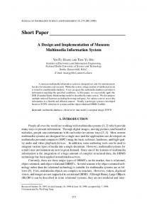
VI. SYSTEM CONFIGURATION AND ANALYSIS OF THE COMPUTATIONAL COMPLEXITY Fig. 2 summarizes the implementation of our speaker-clustering system. In the absence of knowing the true speaker population size, the system in turn hypothesizes that N utterances to be clustered can be from one speaker, two speakers, . . ., or N speakers. For each of the possible speaker population sizes, MDC is run with the number of clusters specified as the hypothesized speaker population size. This yields N partitionings optimized by GA, along with N BIC-motivated scores. The system then outputs the partitioning associated with the largest BIC-motivated score. In view of the usability, it is worth comparing the computational complexity of the proposed clustering system with that of a GLR-based hierarchical clustering system. We observe that there are two factors which dominate the overall computational time for both systems. The first factor arises from the Gaussian mixture modeling of feature vectors, e.g., the generation of λnk in Eq. (1), or the generation of cluster model λ(m) in Eq. (25). The second factor arises from the computation of Gaussian functions based on the models, e.g., Pr(Xn |λnk ), or S(λ(m) , λn ). However, if the models are generated using the MAP adaptation, the first factor can be ignored, compared to the second factor. Hence, the system complexity depends mainly on how many Gaussian functions need to be performed. Consider an agglomerative hierarchical clustering system, in which the inter-cluster similarities are measured on an utterance-concatenation basis. If the system has generated M + 1 clusters c1 , c2 , . . . , cM +1 , and is going to determine which pair of clusters can be merged, it requires to compute M likelihood probabilities for every “long utterance” formed by concatenating all the utterances within a cluster. The likelihood probability is concerned with the term Pr(Xn |λnk ) in Eq. (1), where Xn represents the long utterance for cn , and λnk represents the GMM trained using two long utterances Xn and Xk . For example, to determine which two among the three long utterances X1 , X2 , and X3 can be merged, the system requires to compute two likelihood probabilities Pr(X1 |λ12 ) and Pr(X1 |λ13 ) for X1 , two likelihood probabilities Pr(X2 |λ12 ) and Pr(X2 |λ23 ) 18
for X2 , and two likelihood probabilities Pr(X3 |λ13 ) and Pr(X3 |λ23 ) for X3 . Note that though Eq. (1) contains another likelihood probability Pr(Xn |λn ), such a term has been computed already in the last merging stage, i.e., merging M + 2 clusters into M + 1 clusters. Therefore, to derive M clusters from M + 1 clusters, the system needs to perform M × J × T Gaussian functions, where J is the number of Gaussian mixtures as denoted earlier, and T is the total number of feature vectors in the utterance collection. To complete a cluster tree with the numbers of clusters ranging from 1 to N , the system requires to perform
P(N −1) M =1
M × J × T = 12 N (N − 1)JT Gaussian functions.
Accordingly, the computational complexity of the GLR-based hierarchical clustering system can be characterized by O
³
1 N (N 2
´
− 1)JT ' O( 12 N 2 JT ).
With regard to the proposed speaker-clustering system, whenever a chromosome is generated for assigning each utterance a cluster index, the system needs to compute N divergency-based similarities S(·). Since S(·) involves J Gaussian functions, optimizing M clusters via GA requires to perform N × J × Z × Q Gaussian functions, where Z and Q are, as denoted earlier, the number of chromosomes and the maximum number of generations, respectively. Thus, to determine the optimal number of clusters, a scan from M = 1 to M = N involves computational complexity around O(N 2 JZQ). We can see that the proposed system requires 2ZQ/T times the computational complexity of the GLR-based hierarchical clustering system. However, if the value of ZQ is set to T /2, the two systems have similar computational complexities.
VII. EXPERIMENTS A. Speech Data Our speech data was extracted from two corpora released by the Linguistic Data Consortium [26]: the 1998 HUB-4 Broadcast News Evaluation English Test Material (Hub4-98), which consists of broadcast news speech recorded at a 16 kHz sampling rate, and the 2001 NIST Speaker Recognition Evaluation Corpus (SRE-01), which consists of cellular telephone speech recorded at an 8 kHz sampling rate. The data was divided into three subsets. The first contained 399 speaker19
homogeneous utterances obtained by segmenting the episode “h4e-98-1” of Hub4-98, according to the annotation file. This subset involved 79 speakers, in which the number of utterances spoken by each speaker ranged from 1 to 48. The second subset contained 428 speaker-homogeneous utterances obtained by also segmenting the episode “h4e-98-2” of Hub4-98, according to the annotation file. There were 89 speakers in this subset, and the number of utterances spoken by each speaker ranged from 1 to 27. The third subset, which stems from the test set of SRE-01, contained 197 speaker-homogeneous utterances spoken by 15 randomly-selected male speakers. The number of utterances spoken by each speaker ranged from 5 to 39. The speaker-clustering methods used in this study were optimized using the utterances in the first subset, and the methods’ performances were then evaluated using the utterances in the second and third subsets. Feature vectors, each consisting of 20 MFCCs, were extracted from these utterances for every 20-ms Hamming-windowed frame with 10-ms frame shifts. Prior to MFCC computation, voice active detection [46] was applied to remove salient non-speech regions that may be included in an utterance. The total non-silence numbers of feature vectors for “h4e-98-1”, “h4e-98-2”, and “SRE-01” were 551,019 frames, 545,700 frames, and 418,625 frames, respectively. B. Performance Evaluation Metrics The performance of speaker clustering was evaluated on the basis of two metrics: cluster purity [1][25][44] and the Rand Index [16][37][44]. Cluster purity is the probability that if we pick any utterance from a cluster twice at random, with replacement, both of the selected utterances are from the same speaker. Specifically, the purity of cluster cm is computed by ρm =
P X n2mp p=1
n2m∗
,
(29)
where nm∗ is the total number of utterances in cluster cm , nmp is the number of utterances in cluster cm produced by the p-th speaker, and P is the total number of speakers. From Eq. (29), it follows that n−1 m∗ ≤ ρm ≤ 1, in which the upper bound and lower bound reflect that all the within-cluster utterances were produced by the same speaker and completely different speakers, 20
respectively. To evaluate the overall performance of M -clustering, we compute an average purity ρ¯ =
M 1 X nm∗ ρm . N m=1
(30)
The Rand Index used in this study follows [44], which indicates the level of disagreement in a partitioning. However, for ease of performance comparison, we represent the disagreement as a probability instead of the number of utterance pairs originally used in [44]. Specifically, the Rand Index is defined by the probability that two randomly-selected utterances from the same speaker are placed in different clusters, or that two randomly-selected utterances placed in the same cluster are from different speakers: M X
R=
n2m∗ +
m=1
P X
n2∗p − 2
p=1 M X n2m∗ m=1
+
M X P X
n2mp
m=1 p=1 P X n2∗p p=1
,
(31)
where n∗p is the number of utterances from the p-th speaker. The lower the value of R, the better the clustering performance. Perfect clustering should produce a Rand Index of zero. Note that the cluster purity and Rand Index defined above are calculated without taking the length of utterance into account. However, in many applications, assigning a long utterance into a wrong cluster can be more detrimental than assigning a short utterance into a wrong cluster. To reflect this matter, we further compute the two metrics on the basis of frame correctness. Specifically, a frame-based cluster purity is defined by the probability that if we pick any frame from a cluster twice at random, with replacement, both of the selected frames are from the same speaker. Thus, when computing a frame-based purity by Eq. (29), nm∗ represents the total number of frames in cluster cm , and nmp represents the number of frames in cluster cm produced by the p-th speaker. Likewise, a frame-based Rand Index is defined by the probability that two randomly-selected frames from the same speaker are placed in different clusters, or that two randomly-selected frames placed in the same cluster are from different speakers. In general, when evaluating a certain clustering result, the value of frame-based purity is larger than that of utterance-based purity, while the value of the frame-based Rand Index is smaller than that of the utterance-based Rand Index. 21
C. Experimental Results Our first experiment was conducted to assess the speaker-clustering performance by assuming that the total number of speakers is known; hence, the required number of clusters can be specified as a priori. Figs. 3 and 4 show the performance of agglomerative hierarchical clustering for subsets “h4e-98-2” and “SRE-01”, respectively, in which the numbers of clusters were specified as 89 and 15. We examined different inter-cluster similarity measures along with GLRs computed with different numbers of component densities in Gaussian mixture modeling. The “Concatenation” in Figs. 3 and 4 stands for the inter-cluster similarity measured by concatenating all the utterances within each cluster into a long utterance, and then computing the GLR between the concatenated utterances. Except for the single-Gaussian models (number of Gaussian mixtures = 1), which were full-covariance structures and trained via maximum likelihood estimation, all the GMMs (number of Gaussian mixtures ≥ 2) used in this study comprised diagonal covariance matrices trained via MAP-adaptation from an utterance-independent GMM. We observe from Figs. 3 and 4 that, of the three linkages, complete linkage performs the best, which almost always yields larger values of purity and smaller values of the Rand Index than those of the others; single linkage performs the worst, and average linkage is between the two extremes. It can also be seen from the figures that “Concatenation” surpasses complete linkage in terms of the largest value of purity and smallest value of the Rand Index that can be produced. However, there was no consistent results that could indicate the optimal number of Gaussian mixtures used in GLR computation. Figs. 5 and 6 show the speaker-clustering results obtained by our proposed methods. Here, “GLR-HC Concatenation” represents “Concatenation” shown in Figs. 3 and 4. In GA optimization, the parameter values used for the maximum number of generations Q, the chromosome population size Z, the crossover probability, and the mutation probability were determined to be 4,000, 200, 0.32, and 0.2, respectively, according to the test on subset “h4e-98-1”. We can see from Figs. 5 and 6 that both MLC and MDC yield larger values of purity and smaller values of the Rand Index than most “GLR-HC Concatenation” cases can attain. Table I summarizes the
22
individual best speaker-clustering performance that MLC, MDC, and “GLR-HC Concatenation” achieved, in which the numbers in parentheses indicate the number of component densities used in Gaussian mixture modeling. It is clear from Table I that the proposed methods are superior to the hierarchical-clustering method. In addition, we observe from Figs. 5 and 6 that the performance of MLC is slightly better than that of MDC. However, as mentioned earlier, MLC is rather computationally extensive, due to the need to compute Gaussian densities frame by frame. Quantitatively, MLC required 2,000 times the computational time of MDC for this clustering task, and took weeks to complete a trial on a 3 GHz Pentium PC. This makes it difficult to use MLC to determine how many clusters should be generated if the number of speakers is not known in advance. Therefore, in the following experiments, we concentrated on examining the validity of MDC-based speaker clustering. Figs. 7 and 8 show the speaker-clustering performance as a function of the number of clusters, in which the numbers of Gaussian mixtures used in subsets “h4e-98-2” and “SRE-01” were 1 and 32, respectively. We can see that the average purity increases as the number of clusters increases. It is also clear from the figures that MDC consistently yields larger values of purity than those obtained with “GLR-HC Concatenation”, regardless of the number of clusters. On the other hand, we observe that the Rand Index decreases with the increase in the number of clusters initially, but increases gradually when too many clusters are generated. In general, the smallest value of the Rand Index occurs when the number of clusters is close to the speaker population size. It can be seen from the figures that the smallest value of Rand Index obtained with MDC is not only smaller than that obtained with “GLR-HC Concatenation” but also located at the number of clusters closer to the true size of speaker population. To investigate if the optimal number of clusters can be determined automatically, we computed the BIC-motivated scores with respect to different numbers of clusters using Eq. (27). Fig. 9 shows the resulting scores obtained with the penalty factor γ set to be equal to, slightly greater than, and slightly smaller than one, respectively. The arrowed peak of each curve in the figures indicates the optimal number of clusters determined by the criterion of Eq. (28). We can see 23
from the figure that most of the peaks appeared near the actual number of speakers, and the scores declined significantly after an excess of clusters was created. In general, the larger the value of penalty factor, the smaller the estimated optimal number of clusters, and vice versa. The results show that the number of speakers in subset “SRE-01” was estimated very well, whereas the number of speakers in subset “h4e-98-2” tends to be underestimated, if the penalty factor is simply set to be one. We speculate that this underestimation is mainly because, among the total 89 speakers in subset “h4e-98-2”, there were 30 speakers who spoke only one utterance, and many of these speakers’ utterances were shorter than five seconds, which leads to the tendency that these speakers are ignored. Despite this, we observe from the figure that such an underestimation can be mitigated using the penalty factor slightly smaller than one. This result validates the proposed method for estimating the speaker population size. We conclude the experiments with a note that, compared to “GLR-HC Concatenation”, the proposed method improves the speaker-clustering performance at the the cost of slightly higher computational requirement. Quantitatively, our system took 2ZQ/T ' 3 times the computational time of “GLR-HC Concatenation”, in which Z = 200, Q = 4, 000, and the total number of feature vectors T was roughly 500,000 frames for all the three subsets. However, as the values of Z and Q are adjustable, the proposed system is more flexible than “GLR-HC Concatenation” in terms of computational complexity.
VIII. CONCLUSIONS This study has investigated methods for partitioning speech utterances into clusters so that the level of homogeneity of within-cluster utterances can be as high as possible. Such homogeneity has been characterized by either the likelihood probability that a cluster model tests for each of the within-cluster utterances, or the divergence-based similarity between a cluster model and each of the within-cluster utterance models. For greater efficiency, both cluster models and utterance models are adapted from a cluster-independent model trained using all the utterances to be clus24
tered. To enable the best partitioning with the maximal amount of within-cluster homogeneity to be found effectively, we have proposed the use of a genetic algorithm to determine the cluster in which each utterance should be placed. Our experimental results show that the proposed method achieves a notable improvement in speaker-clustering performance, compared to the conventional method using GLR-based similarity measurement followed by agglomerative hierarchical clustering. In addition, the proposed clustering method adapts the Bayesian information criterion to determine how many clusters should be generated. The experimental results show that the automatically-determined number of clusters approximates the actual speaker population size. To be of more practical use, our future work will extend the current speaker-clustering methods to deal with speech data containing multiple speakers. This could be done by either assigning each utterance to multiple related clusters [30], or pre-segmenting utterances into small speakerhomogeneous regions and then clustering those regions. In parallel, speaker segmentation may be improved with the aid of speaker clustering [31]. Specifically, speech segments assigned to each cluster can be used to train a speaker-related model, thereby examining the speaker change boundaries of an audio recording in a manner of frame-by-frame recognition. Speaker clustering can then be performed on the updated speech segments, and the segmentation and clustering procedures repeated iteratively to attain the goal of speaker diarization. On the other hand, recognizing the high computational complexity of the proposed speaker-clustering system, more work is still needed to study the way to improve the system efficiency.
ACKNOWLEDGMENTS This work was supported in part by the National Science Council, Taiwan, ROC, under Grant No. NSC93-2213-E-001-017. The authors are very grateful to the anonymous reviewers and the associate editor, Dr. Douglas O’Shaughnessy, for their careful reading of this article and their constructive suggestions.
25
References [1] Ajmera, J., Bourlard, H., Lapidot, I., and McCowan, I. “Unknown-multiple speaker clustering using HMM,” Proc. International Conference on Spoken Language Processing (ICSLP), 2002. [2] Baker, J. E. “Adaptive selection methods for genetic algorithm,” Proc. International Conference on Genetic Algorithms and Their Applications, 1985. [3] Ben, M., Betser, M., Bimbot, F., and Gravier, G. “Speaker diarization using bottom-up clustering based on a parameter-derived distance between adapted GMMs,” Proc. International Conference on Spoken Language Processing (ICSLP), 2004. [4] Bimbot, F., Magrin-Chagnolleau, I., and Mathan, L. “Second-order statistical measures for textindependent speaker identification,” Speech Communication, 17:177-192, 1995. [5] Campbell, J. P. “Speaker recognition:
a tutorial,” PROCEEDINGS OF THE IEEE,
85(9):1437-1462, 1997. [6] Chen, S. S., and Gopalakrishnan, P. S. “Clustering via the Bayesian information criterion with applications in speech recognition,” Proc. IEEE International Conference on Acoustics, Speech, and Signal Processing (ICASSP), 1998. [7] Dempster, A., Laird, N., and Rubin, D. “Maximum likelihood from incomplete data via the EM algorithm,” Journal of the Royal Statistical Society, 1977. [8] Faltlhauser, R., and Ruske, G. “Robust speaker clustering in eigenspace,” Proc. IEEE Workshop on Automatic Speech Recognition and Understanding, 2001. [9] Furui, S. “Unsupervised speaker adaptation method based on hierarchical spectral clustering,” Proc. IEEE International Conference on Acoustics, Speech, and Signal Processing (ICASSP), 1989.
26
[10] Furui, S. “Cepstral analysis technique for automatic speaker verification,” IEEE Transactions on Speech and Audio Processing, 29(2):254-272, 1996. [11] Gish, H. “Robust discrimination in automatic speaker identification,” Proc. IEEE International Conference on Acoustics, Speech, and Signal Processing (ICASSP), 1990. [12] Gish, H., Siu, M. H., and Rohlicek, R. “Segregation of speakers for speech recognition and speaker identification,” Proc. IEEE International Conference on Acoustics, Speech, and Signal Processing (ICASSP), 1991. [13] Goldberg, D. E. Genetic Algorithm in Search, Optimization and Machine Learning. New York: Addison-Wesley, 1989. [14] Hermansky, H., Morgan, N., Bayya, A., and Kohn, P. “Compensation for the effects of the communication channel in auditory-like analysis of speech,” Proc. European Conference on Speech Communication and Technology (Eurospeech), 1991. [15] Huang, C. S., Wang, H. C., Lee, C. H. “A study on model-based error rate estimation for automatic speech recognition”, IEEE Transactions on Speech and Audio Processing, 11(6):581-589, 2003. [16] Hubert, L., and Arabie, P. “Comparing Partitions,” Journal of Classification, 2:193-218, 1985. [17] Jin, H., Kubala, F., and Schwartz, R. “Automatic speaker clustering,” Proc. DARPA Speech Recognition Workshop, 1997. [18] Johnson, S. E. “Who spoke when? - Automatic segmentation and clustering for determining speaker turns,” Proc. European Conference on Speech Communication and Technology (Eurospeech), 1999. [19] Johnson, S. E., and Woodland, P. C. “Speaker clustering using direct maximisation of the MLLR-adapted likelihood,” Proc. International Conference on Spoken Language Processing (ICSLP), 1998. 27
[20] Kaufman, L., and Rousseuw, P. J. Finding Groups in Data: An Introduction to Cluster Analysis. New York: Wiley, 1990. [21] Kosaka, T., and Sagayama, S. “Tree-structured speaker clustering for fast speaker adaptation,” Proc. IEEE International Conference on Acoustics, Speech, and Signal Processing (ICASSP), 1994. [22] Kullback, S. Information Theory and Statistics. New York: Dover, 1968. [23] Kwon, S., and Narayanan, S. “Unsupervised speaker indexing using generic models,” IEEE Transactions on Speech and Audio Processing, 13(5):72-83, 2005. [24] Lapidot, I., Guterman, H., and Cohen, A. “Unsupervised speaker recognition based on competition between self-organizing maps,” IEEE Transactions on Neural Networks, 13(4):877-887, 2002. [25] Lapidot, I. “SOM as likelihood estimator for speaker clustering,” Proc. European Conference on Speech Communication and Technology (Eurospeech), 2003. [26] LDC, http://www.ldc.upenn.edu/ [27] Liu, D., and Kubala, F. “Online speaker clustering,” Proc. IEEE International Conference on Acoustics, Speech, and Signal Processing (ICASSP), 2003. [28] Liu, Z. “An efficient algorithm for clustering short spoken utterances”, Proc. IEEE International Conference on Acoustics, Speech, and Signal Processing (ICASSP), 2005. [29] Makhoul, J., Kubala, F., Leek, T., Liu, D., Nguyen, L., Schwartz, R., and Srivastava, A. “Speech and language technologies for audio indexing and retrieval,” PROCEEDINGS OF IEEE, 88(8):1338- 1353, 2000. [30] McLaughlin, J., Reynolds, D., Singer, E., and O’Leary, G. C. “Automatic speaker clustering from multi-speaker utterances,” Proc. IEEE International Conference on Acoustics, Speech, and Signal Processing (ICASSP), 1999. 28
[31] Moraru, D., and Meignier, S. “The ELISA consortium approaches in broadcast news speaker segmentation during the NIST 2003 Rich Transcription Evaluation,” Proc. IEEE International Conference on Acoustics, Speech, and Signal Processing (ICASSP), 2004. [32] Moh, Y., Nguyen, P., and Junqua, J. C. “Towards domain independent speaker clustering,” Proc. IEEE International Conference on Acoustics, Speech, and Signal Processing (ICASSP), 2003. [33] NIST, “Benchmark Tests: Speaker Recognition,” http://www.nist.gov/speech/tests/spk/ 2001/index.htm [34] NIST, “Benchmark Tests:
Rich Transcription,” http://www.nist.gov/speech/tests/rt/
rt2005/spring/index.htm [35] O’Shaughnessy, D. “Speaker Recognition,” IEEE ASSP Magazine, 1986. [36] Pelecanos, J., and Sridharan, S. “Feature warping for robust speaker verification,” Proc. ISCA Odyssey Workshop, 2001. [37] Rand, W. M. “Objective criteria for the evaluation of clustering methods,” Journal of the American Statistical Association, 66:846-850, 1971. [38] Reynolds, D. A., Quatieri, T. F., and Dunn, R. B. “Speaker verification using adapted Gaussian mixture models,” Digital Signal Processing, 10:19-41, 2000. [39] Reynolds D. A., and Rose, R. C. “Robust text-independent speaker identification using Gaussian mixture speaker models,” IEEE Transactions on Speech and Audio Processing, 3(1):72-83, 1995. [40] Reynolds, D. A., Singer, E., Carson, B. A., O’Leary, G. C., McLaughlin, J. J., and Zissman, M. A. “Blind clustering of speech utterances based on speaker and language characteristics,” Proc. International Conference on Spoken Language Processing (ICSLP), 1998.
29
[41] Schwarz, G. “Estimating the Dimension of a Model,” The Annals of Statistics 6:461-464, 1978. [42] Siegler, M. A., Jain, U., Raj, B., and Stern, R. M. “Automatic segmentation, classification and clustering of broadcast news audio,” Proc. DARPA Speech Recognition Workshop, 1997. [43] Sinha, R., Tranter, S. E., Gales, M. J. F., and Woodland, P. C. “The Cambridge University March 2005 Speaker Diarisation System,” Proc. European Conference on Speech Communication and Technology (Eurospeech), 2005. [44] Solomonoff, A., Mielke, A., Schmidt, M., and Gish, H. “Clustering speakers by their voices,” Proc. IEEE International Conference on Acoustics, Speech, and Signal Processing (ICASSP), 1998. [45] Tranter, S. E. “Two-way Cluster Voting to Improve Speaker Diarisation Performance,” Proc. IEEE International Conference on Acoustics, Speech, and Signal Processing (ICASSP), 2005. [46] The VIMAS speech codec, http://www.vimas.com [47] Zhou, B., and Hansen, J. H. L. “Unsupervised audio stream segmentation and clustering via the Bayesian information criterion,” Proc. International Conference on Spoken Language Processing (ICSLP), 2000. [48] Zhu, X., Barras, C., Meignier, S., and Gauvain, J. L. “Combining speaker identification and BIC for speaker diarization,” Proc. European Conference on Speech Communication and Technology (Eurospeech), 2005.
30
TABLE I. Summary of Figs. 4 and 5, in which the individual best speaker-clustering performance that MLC, MDC, and “GLR-HC Concatenation” achieved is listed. The numbers in parentheses indicate the number of component densities used in Gaussian mixture modeling. (a) Results of clustering subset “h4e-98-2” Clustering Method Evaluation Metric
MLC
MDC
GLR-HC Concatenation
Utterance-based Purity
0.80 (1)
0.80 (1)
0.74 (1)
Frame-based Purity Utterance-based Rand Index Frame-based Rand Index
0.88 (1) 0.30 (1) 0.19 (2)
0.86 (1) 0.31 (1) 0.21 (2)
0.84 (1) 0.37 (1) 0.19 (4)
(b) Results of clustering subset “SRE-02” Clustering Method Evaluation Metric Utterance-based Purity Frame-based Purity Utterance-based Rand Index Frame-based Rand Index
MLC
MDC
GLR-HC Concatenation
0.76 (32) 0.81 (32) 0.27 (32) 0.24 (32)
0.75 (32) 0.79 (32) 0.27 (32) 0.23 (32)
0.67 (1) 0.73 (1) 0.38 (32) 0.28 (32)
31
Start Initialization Fitness Evaluation Selection Crossover Mutation No Terminate ? Yes Stop
FIG. 1. Flow diagram of the genetic algorithm.
N Utterances
Forming 1 cluster
Computing (1)
Forming 2 clusters
Computing (2)
Forming N clusters
Computing (N)
Picking maximum
M* Clusters
Minimum Divergency Clustering Forming utterance GMMs λ1, λ2, ..., λN MAP adaptation N Utterances X1, X2, ..., XN
Forming cluster-independent GMM λ MAP adaptation
Assigning Xn a cluster index gn
1≤ n ≤ N
Forming cluster GMMs λ(1) and λ(2)
2
N
Computing
∑∑ log S (λ m =1 n =1
(m)
, λ n )δ (g n , m)
Generating/modifying the cluster indices via GA * * * Optimal cluster indices g 1 , g 2 ,..., g N
FIG. 2. Block diagram of the proposed speaker-clustering system.
32
Complete Linkage
Average Linkage
Average Linkage
Single Linkage
Single Linkage
Concatenation
1.00
Concatenation
1.00
0.90
0.90
0.80
0.80
Frame-based Purity
Utterance-based Purity
Complete Linkage
0.70 0.60 0.50 0.40
0.70 0.60 0.50 0.40 0.30
0.30
0.20
0.20
1
2
4
8
16
1
32
(a) Utterance-based Purity
8
16
32
Complete Linkage
Complete Linkage
Average Linkage
Average Linkage
Single Linkage
Single Linkage Concatenation
1.00
0.90
0.90
Frame-based Rand Index
Utterance-based Rand Index
4
(b) Frame-based Purity
Concatenation
1.00
2
No. of Gaussian Mixtures
No. of Gaussian Mixtures
0.80 0.70 0.60 0.50 0.40 0.30 0.20
0.80 0.70 0.60 0.50 0.40 0.30 0.20
0.10
0.10
1
2
4
8
16
32
1
No. of Gaussian Mixtures
2
4
8
16
32
No. of Gaussian Mixtures
(c) Utterance-based Rand Index
(d) Frame-based Rand Index
FIG. 3. Performance of agglomerative hierarchical clustering for subset “h4e-98-2”, in which the number of clusters was specified as the true size of speaker population, i.e., 89. Except for the single-Gaussian models (No. of Gaussian Mixtures = 1), which were full-covariance structures and trained via maximum likelihood estimation, all the GMMs (No. of Gaussian Mixtures ≥ 2) comprised diagonal covariance matrices trained via MAP adaptation.
33
Complete Linkage
Average Linkage
Average Linkage
Single Linkage
Single Linkage
Concatenation
1.00
Concatenation
1.00
0.90
0.90
0.80
0.80
Frame-based Purity
Utterance-based Purity
Complete Linkage
0.70 0.60 0.50 0.40
0.70 0.60 0.50 0.40
0.30
0.30
0.20
0.20 0.10
0.10
1
2
4
8
16
1
32
(a) Utterance-based Purity
8
16
32
Complete Linkage
Complete Linkage
Average Linkage
Average Linkage
Single Linkage
Single Linkage Concatenation
1.00
0.90
0.90
Frame-based Rand Index
Utterance-based Rand Index
4
(b) Frame-based Purity
Concatenation
1.00
2
No. of Gaussian Mixtures
No. of Gaussian Mixtures
0.80 0.70 0.60 0.50 0.40 0.30
0.80 0.70 0.60 0.50 0.40 0.30
0.20 0.10
0.20
1
2
4
8
16
32
1
No. of Gaussian Mixtures
2
4
8
16
32
No. of Gaussian Mixtures
(c) Utterance-based Rand Index
(d) Frame-based Rand Index
FIG. 4. Performance of agglomerative hierarchical clustering for subset “SRE-02”, in which the number of clusters was specified as the true size of speaker population, i.e., 15. Except for the single-Gaussian models (No. of Gaussian Mixtures = 1), which were full-covariance structures and trained via maximum likelihood estimation, all the GMMs (No. of Gaussian Mixtures ≥ 2) comprised diagonal covariance matrices trained via MAP adaptation.
34
1.00
0.90
0.90
0.80
0.80
Frame-based Purity
Utterance-based Purity
1.00
0.70 0.60 0.50 MLC
0.40
MDC
0.30
0.70 0.60 0.50 MLC
0.40
MDC
0.30
GLR-HC Concatenation
0.20
GLR-HC Concatenation
0.20
1
2
4
8
16
32
1
No. of Gaussian Mixtures
8
16
32
(b) Frame-based Purity 1.00
MLC
0.90
MDC
0.80
GLR-HC Concatenation
Frame-based Rand Index
Utterance-based Rand Index
4
No. of Gaussian Mixtures
(a) Utterance-based Purity 1.00
2
0.70 0.60 0.50 0.40 0.30 0.20
MLC
0.90
MDC
0.80
GLR-HC Concatenation
0.70 0.60 0.50 0.40 0.30 0.20
0.10
0.10
1
2
4
8
16
32
1
No. of Gaussian Mixtures
2
4
8
16
32
No. of Gaussian Mixtures
(c) Utterance-based Rand Index
(d) Frame-based Rand Index
FIG. 5. Performance of the proposed maximum likelihood clustering (MLC) and minimum divergence clustering (MDC) for subset “h4e-98-2”, in which “GLR-HC Concatenation” represents “Concatenation” shown in Figs. 2.
35
1.00
0.90
0.90
0.80
0.80
Frame-based Purity
Utterance-based Purity
1.00
0.70 0.60 0.50 MLC
0.40
MDC
0.30
0.70 0.60 0.50 MLC
0.40
MDC
0.30
GLR-HC Concatenation
0.20
GLR-HC Concatenation
0.20
1
2
4
8
16
32
1
No. of Gaussian Mixtures
8
16
32
(b) Frame-based Purity 1.00
MLC
0.90
MDC
0.80
GLR-HC Concatenation
Frame-based Rand Index
Utterance-based Rand Index
4
No. of Gaussian Mixtures
(a) Utterance-based Purity 1.00
2
0.70 0.60 0.50 0.40 0.30 0.20
MLC
0.90
MDC
0.80
GLR-HC Concatenation
0.70 0.60 0.50 0.40 0.30 0.20
0.10
0.10
1
2
4
8
16
32
1
No. of Gaussian Mixtures
2
4
8
16
32
No. of Gaussian Mixtures
(c) Utterance-based Rand Index
(d) Frame-based Rand Index
FIG. 6. Performance of the proposed maximum likelihood clustering (MLC) and minimum divergence clustering (MDC) for subset “SRE-02”, in which “GLR-HC Concatenation” represents “Concatenation” shown in Figs. 3.
36
1.00
0.90
0.90
0.80
0.80
Frame-based Purity
Utterance-based Purity
1.00
0.70 0.60 0.50 0.40
0.70 0.60 0.50 0.40
MDC
0.30
MDC
0.30
GLR-HC Concatenation
0.20
0.20 20
40
60
80 100 120 140 160 180 200 Number of Clusters
20
(a) Utterance-based Purity
40
60
80 100 120 140 160 180 200 Number of Clusters
(b) Frame-based Purity
0.70
0.70 MDC
0.65
MDC
0.65
GLR-HC Concatenation
GLR-HC Concatenation
Frame-based Rand Index
Utterance-based Rand Index
GLR-HC Concatenation
0.60 0.55 0.50 0.45 0.40 0.35
0.60 0.55 0.50 0.45 0.40 0.35 0.30 0.25
0.30
0.20 20
40
60
80 100 120 140 160 180 200 Number of Clusters
20
(c) Utterance-based Rand Index
40
60
80 100 120 140 160 180 200 Number of Clusters
(d) Frame-based Rand Index
FIG. 7. Performance of clustering subset “h4e-98-2” as a function of the number of clusters, in which the number of component densities used in Gaussian mixture modeling was 1 (single-Gaussian model with full covariance matrix).
37
1.00
0.90
0.90
0.80
0.80
Frame-based Purity
Utterance-based Purity
1.00
0.70 0.60 0.50 0.40
0.70 0.60 0.50 0.40
0.30
MDC
0.30
MDC
0.20
GLR-HC Concatenation
0.20
GLR-HC Concatenation
0.10
0.10 5
10 15 20 25 30 35 40 45 50 55 Number of Clusters
5
(a) Utterance-based Purity
(b) Frame-based Purity
1.00
1.00 MDC
0.90
MDC
0.90
GLR-HC Concatenation
GLR-HC Concatenation
Frame-based Rand Index
Utterance-based Rand Index
10 15 20 25 30 35 40 45 50 55 Number of Clusters
0.80 0.70 0.60 0.50 0.40 0.30 0.20
0.80 0.70 0.60 0.50 0.40 0.30 0.20
0.10
0.10 5
10 15 20 25 30 35 40 45 50 55 Number of Clusters
5
(c) Utterance-based Rand Index
10 15 20 25 30 35 40 45 50 55 Number of Clusters
(d) Frame-based Rand Index
FIG. 8. Performance of clustering subset “SRE-02” as a function of the number of clusters, in which the number of component densities used in Gaussian mixture modeling was 32.
38
-200.00 -220.00
BIC-motivated Scores
-240.00
γ = 0.7
-260.00 -280.00 -300.00 -320.00 -340.00 -360.00
γ = 1.0 Speaker Population Size = 89
γ = 1.2
-380.00 20 40 60 80 100 120 140 160 180 200 Number of Clusters
(a) Tests on subset “h4e-98-2”.
-190.00 -195.00
γ = 0.7
-200.00
BIC-motivated Scores
-205.00 -210.00 -215.00 -220.00 -225.00
γ = 1.0
-230.00 -235.00 -240.00 -245.00
Speaker Population Size = 15
-250.00
γ = 1.2
3 6 9 12 15 18 21 24 27 30 33 36 39 Number of Clusters
(b) Tests on subset “SRE-02”. FIG. 9. BIC-motivated scores as a function of number of clusters, in which the penalty factor γ was set to be equal to, slightly greater than, and slightly smaller than one, respectively. The arrowed peak of each curve indicates the optimal number of clusters according to the criterion in Eq. (28).
39