Incremental Method for Spectral Clustering of Increasing Orders

Incremental Method for Spectral Clustering of Increasing Orders∗ Pin-Yu Chen†

Baichuan Zhang‡

Mohammad Al Hasan‡

arXiv:1512.07349v1 [cs.SI] 23 Dec 2015

Abstract The smallest eigenvalues and the associated eigenvectors (i.e., eigenpairs) of a graph Laplacian matrix have been widely used for spectral clustering and community detection. However, the majority of applications require computation of a large number Kmax of eigenpairs, where Kmax is an upper bound on the number K of clusters, called the order of the clustering algorithms. In this work, we propose an incremental method for constructing the eigenspectrum of the graph Laplacian matrix. This method leverages the eigenstructure of graph Laplacian matrix to obtain the k-th eigenpairs of the Laplacian matrix given a collection of all the k − 1 smallest eigenpairs. Our proposed method adapts the Laplacian matrix such that the batch eigenvalue decomposition problem transforms into an efficient sequential leading eigenpair computation problem. As a practical application of our proposed method, we consider user-guided spectral clustering. Specifically, we demonstrate that users can utilize the proposed incremental method for effective eigenpair computation and determining the desired number of clusters based on multiple clustering metrics.

1 Introduction Over the past two decades, the graph Laplacian matrix and its variants have been widely adopted for solving various research tasks, including graph partitioning [21], data clustering [13], community detection [4, 26], consensus in networks [18], dimensionality reduction [2], entity disambiguation [29], graph signal processing [25], centrality measures for graph connectivity [3], interconnected physical systems [22], network vulnerability assessment [6], image segmentation [24], among others. The fundamental task is to represent the data of interest as a graph for analysis, where a node represents an entity (e.g., a pixel or a user in a social network) and ∗ This work is partially supported by the Consortium for Verification Technology under Department of Energy National Nuclear Security Administration award number de-na0002534, by ARO grant W911NF-15-1-0479, by ARO grant W911NF-15-10241, and by Mohammad Hasan’s NSF CAREER Award (IIS1149851). † Department of Electrical Engineering and Computer Science, Univervity of Michigan, Ann Arbor, USA ‡ Department of Computer and Information Science, Indiana University - Purdue University Indianapolis, USA

Alfred O. Hero III†

an edge represents similarity (e.g., a distance metric between two multivariate data samples) or actual relation (e.g., friendship) between nodes [13]. More often the K eigenvectors associated with the K smallest eigenvalues of the graph Laplacian matrix are used to cluster the entities into K clusters of high similarity. For brevity, throughout this paper we will call these eigenvectors as the K smallest eigenvectors. The success of graph Laplacian matrix based methods for graph partitioning and spectral clustering can be explained by the fact that acquiring K smallest eigenvectors is equivalent to solving a relaxed graph cut minimization problem, which partitions a graph into K clusters by minimizing various objective functions including min cut, ratio cut or normalized cut [13]. Generally, in clustering, K is selected to be much smaller than n (the number of data points), making full eigen decomposition (such as, Cholesky factorization, or Schur Decomposition) unnecessary. An efficient alternative is to use methods that are based on power iteration, such as Arnoldi method or Lanczos method, which computes the leading eigenpair through repeated matrix vector multiplication. Subsequent eigenpairs can be obtained by finding the leading eigenvector in the null space of the given Laplacian matrix. ARPACK [12] library is a popular parallel implementation of different variants of Arnoldi and Lanczos method, which is used by many commercial software including Matlab. However, in most situations the best value of K is unknown and a heuristic is used to determine the number of clusters, e.g., fixing a maximum number of clusters Kmax and detecting a large gap in the values of the Kmax largest sorted eigenvalues or normalized cut score [15, 19]. Sometimes, this value of K can be determined based on domain knowledge [1]. For example, a user may require that the largest cluster size be no more than 10% of the total number of nodes or that the total inter-cluster edge weight be no greater than a certain amount. In these cases, the desired choice of K cannot be determined a priori. Over-estimation of the upper bound Kmax on the number K of clusters is expensive as the cost of finding K eigenpairs using the power iteration method grows rapidly with K. On the other hand, choosing an insufficiently large value for Kmax runs the risk of severe bias. Setting Kmax to the

number of data points n is generally computationally infeasible, even for a moderate-sized graph. Therefore, an incremental eigenpair computation method that effectively computes the K-th smallest eigenpair of graph Laplacian matrix by utilizing the previously computed K − 1 smallest eigenpairs is needed. Such an iterative method obviates the need to set an upper bound Kmax on K, and its efficiency can be explained by the adaptivity to increments in K. In this work, we propose an efficient method for incremental computation of smallest eigenvalues and eigenvectors (i.e., smallest eigenpairs) by exploiting the eigenspace structure of graph Laplacian matrices. For each increment, given the previously computed smallest eigenpairs, we show that computing the next smallest eigenpair is equivalent to computing a leading eigenpair of a particular matrix, which transforms potentially tedious numerical computation (such as the tridiagonalization step in Lanczos algorithm [11]) to simple matrix power iterations of known computational efficiency [11]. Our experimental results show that for a given K, the proposed incremental computation provides a significant reduction in computation time compared to a batch computation method which computes the K smallest eigenpairs in a single batch. Also, as K increases, the gap between the incremental approach and the batch approach widens, providing an order of magnitude speed-up. As a demonstration, we apply the incremental computation method to design a user-guided spectral clustering algorithm, which provides clustering solution for a sequence of K values and updates multiple cluster quality metrics for facilitating the selection of final clustering. The contributions of this paper are summarized as follows. 1. We propose an incremental eigenpair computation method for both unnormalized and normalized graph Laplacian matrices, by transforming the original eigenvalue decomposition problem into an efficient sequential leading eigenpair computation problem. Simulation results show that the proposed method has superior performance over the batch computation method in terms of computation time. To the best of our knowledge, this is the first method for incremental eigenpair computation for graph Laplacian matrices. 2. We use several real-life datasets to demonstrate the utility of the proposed incremental eigenpair computation method. Specifically, we show that the proposed method is suitable for user-guided spectral clustering which provides a sequence of clustering results for unit increment of the number K of clusters, and updates the associated cluster

evaluation metrics for helping a user in decision making. 2

Related Works

2.1 Incremental eigenvalue decomposition The proposed method aims to incrementally compute the smallest eigenpair of a given graph Laplacian matrix. There are several works that are named as incremental eigenvalue decomposition methods [7, 9, 16, 17, 23]. However, these works focus on updating the eigenstructure of graph Laplacian matrix of dynamic graphs when nodes (data samples) or edges are inserted or deleted into the graph. 2.2 Cluster Count Selection for Spectral Clustering Many spectral clustering algorithms utilize the eigenstructure of graph Laplacian matrix for selecting number of clusters. In [19], a value K that maximizes the gap between the K-th and the (K +1)-th smallest eigenvalue is selected as the number of clusters. In [15], a value K that minimizes the sum of cluster-wise Euclidean distance between each data point and the centroid obtained from K-means clustering on K smallest eigenvectors is selected as the number of clusters. In [28], the smallest eigenvectors of normalized graph Laplacian matrix are rotated to find the best alignment that reflects the true clusters. A model based method for determining the number of clusters is proposed in [20]. Note that aforementioned methods use only one single clustering metric to determine the number of clusters and often implicitly assume an upper bound on K (namely Kmax ). 3

Incremental Eigenpair Computation Graph Laplacian Matrices

for

3.1 Background Throughout this paper bold uppercase letters (e.g., X) denote matrices and Xij (or [X]ij ) denotes the entry in i-th row and j-th column of X, bold lowercase letters (e.g., x or xi ) denote column vectors, (·)T denotes matrix or vector transpose, italic letters (e.g., x or xi ) denote scalars, and calligraphic uppercase letters (e.g., X or Xi ) denote sets. The n × 1 vector of ones (zeros) is denoted by 1n (0n ). The matrix I denotes an identity matrix and the matrix O denotes the matrix of zeros. We use two n × n symmetric matrices, A and W, to denote the adjacency and weight matrices of an undirected weighted simple graph G with n nodes and m edges. Aij = 1 if there is an edge between nodes i and j, and Aij = 0 otherwise. W is a nonnegative symmetric matrix such that Wij P ≥ 0 if Aij = 1 and Wij = 0 n if Aij = 0. Let si = j=1 Wij denote the strength

Graph Type / Graph Laplacian Matrix Connected Graphs Disconnected Graphs

Unnormalized Lemma 3.1, Theorem 3.1 Lemma 3.2, Theorem 3.2

Normalized Corollary 3.1, Corollary 3.3 Corollary 3.2, Corollary 3.4

Table 1: Utility of the established lemmas, corollaries, and theorems. of node i. Note that when W = A, the strength of a node is equivalent to its degree. S = diag(s1 , s2 , . . . , sn ) is a diagonal matrix with nodal strength on its main diagonal and the off-diagonal entries being zero. The (unnormalized) graph Laplacian matrix is defined as (3.1)

L = S − W.

(3.3)

One popular variant of the graph Laplacian matrix is the normalized graph Laplacian matrix defined as (3.2)

LN = S

− 12

LS

− 12

=I−S

Proof. Since L is a positive semidefinite (PSD) matrix, λi (L) ≥ 0 for all i. Since G is a connected graph, by (3.1) L1n = (S − W)1n = 0n . Therefore, by the PSD 1n property we have (λ1 (L), v1 (L)) = (0, √ ). Moreover, n since L is a symmetric real-valued square matrix, from (3.1) we have

− 21

WS

− 12

,

1

trace(L) =

n X

Lii =

n X

λi (L) =

si = s.

i=1

i=1

i=1

n X

By the PSD property of L, we have λn (L) < s since λ2 (L) > 0 for any connected graph. Therefore, by the orthogonality of eigenvectors of L (i.e., 1Tn vi (L) = 0 e can be for all i ≥ 2) the eigenvalue decomposition of L represented as

where S− 2 = diag( √1s1 , √1s2 , . . . , √1sn ). The i-th smallest eigenvalue and its associated unitn norm eigenvector of L are denoted by λi (L) and vi (L), X s e λi (L)vi (L)viT (L) + 1n 1Tn L = respectively. That is, the eigenpair (λi , vi ) of L has the n i=2 relation Lvi = λi vi , and λ1 (L) ≤ λ2 (L) ≤ . . . ≤ λn (L). n X The eigenvectors have unit Euclidean norm and they are e i (L)v e T (L), e (3.4) λi (L)v = T i orthogonal to each other such that vi vj = 1 if i = j i=1 and viT vj = 0 if i 6= j. The eigenvalues of L are said 1n to be distinct if λ1 (L) < λ2 (L) < . . . < λn (L). Similar where (λn (L), e vn (L)) e = (s, √ e vi (L)) e = ) and (λi (L), n notations are used for LN . (λi+1 (L), vi+1 (L)) for 1 ≤ i ≤ n − 1. 3.2 Theoretical foundations of the Proposed Method The following lemmas and corollaries provide the cornerstone for establishing the incremental computation method. The main idea is that we utilize the eigenspace structure of graph Laplacian matrix to inflate specific eigenpairs via a particular perturbation matrix, without affecting other eigenpairs. The proposed method works for both connected, and disconnected graphs using both normalized and unnormalized graph Laplacian matrices. To assist the readers in following the proofs, in Table 1 we group the established lemmas, corollaries, and theorems under different graph types and different graph Laplacian matrices. The proofs of Lemma and Theorem for the disconnected graphs are given in the supplementary file. Lemma 3.1. Assume that G is a connected graph and L is the graph Laplacian with si denoting the sum of the entries in the i-th row of the weight matrix W. Let s = Pn e = L+ s 1n 1T . Then the eigenpairs s and define L i n i=1 n e satisfy (λi (L), e vi (L)) e of L = (λi+1 (L), vi+1 (L)) for 1n e vn (L)) e = (s, √ ). 1 ≤ i ≤ n − 1 and (λn (L), n

Corollary 3.1. For a normalized graph Laplacian matrix LN , assume G is a connected graph and let e N ), vi (L e N )) = e N = LN + 2 S 21 1n 1T S 21 . Then (λi (L L n s (λi+1 (LN ), vi+1 (LN )) for 1 ≤ i ≤ n − 1 and 1 2 1n e N ), vn (L e N )) = (2, S√ (λn (L ). s

1

1

Proof. Recall from (3.2) that LN = S− 2 LS− 2 , and also 1 1 we have LN S 2 1n = S− 2 L1n = 0n . Moreover, it can be shown that 0 ≤ λ1 (LN ) ≤ λ2 (LN ) ≤ . . . ≤ λn (LN ) ≤ 2 [14], and λ2 (LN ) > 0 if G is connected. Following the same derivation for Lemma 3.1 we obtain the √ √ √ 1 corollary. Note that S 2 = diag( s1 , s2 , . . . , sn ) and 1 1 (S 2 1n )T S 2 1n = 1Tn S1n = s.

Lemma 3.2. Assume that G is a disconnected Pngraph with δ ≥ 2 connected components, and let s = i=1 si , e = L+ let V = [v1 (L), v2 (L), . . . , vδ (L)], and let L T e e sVV . Then (λi (L), vi (L)) = (λi+δ (L), vi+δ (L)) for e = s for n − δ + 1 ≤ i ≤ n, and 1 ≤ i ≤ n − δ, λi (L) e e . . . , vn (L)] e = V. [vn−δ+1 (L), vn−δ+2 , (L),

Proof. The proof can be found in the supplementary file.

Corollary 3.2. For a normalized graph Laplacian matrix LN , assume G is a disconnected graph with δ ≥ 2 connected components. Let Vδ = [v1 (LN ), v2 (LN ), . . . , vδ (LN )], and let e N = LN + 2Vδ VT . Then (λi (L e N ), vi (L e N )) = L δ (λi+δ (LN ), vi+δ (LN )) for 1 ≤ i ≤ n − δ, e N ) = 2 for n − δ + 1 ≤ i ≤ n, and λi (L e N ), vn−δ+2 , (L e N ), . . . , vn (L e N )] = Vδ . [vn−δ+1 (L Proof. The proof is given in the supplementary file.

Remark 1. The columns of any matrix V′ = VR with an orthonormal transformation matrix R (i.e., e and RT R = I) are also the largest δ eigenvectors of L e N in Lemma 3.2 and Corollary 3.2. Without loss L of generality we consider the case R = I. 3.3 Incremental computation method Given the K smallest eigenpairs of a graph Laplacian matrix, we prove that computing the (K +1)-th smallest eigenpair is equivalent to computing the leading eigenpair (the eigenpair with the largest eigenvalue in absolute value) of a certain perturbed matrix. The advantage of this transformation is that the leading eigenpair can be efficiently computed via matrix power iteration methods [11, 12]. Let VK = [v1 (L), v2 (L), . . . , vK (L)] be the matrix with columns being the K smallest eigenvectors of L and let ΛK = diag(s − λ1 (L), s − λ2 (L), . . . , s − λK (L)) be the diagonal matrix with {s − λi (L)}K i=1 being its main diagonal. The following theorems show that given the K smallest eigenpairs of L, the (K + 1)-th smallest eigenpair of L is the leading eigenvector of the original graph Laplacian matrix perturbed by a certain matrix.

with the originally paired eigenvectors. Using (3.5) we e as obtain the eigenvalue decomposition of L e = L + VK ΛK VT + s 1n 1T − sI L n K n n X (3.6) (λi (L) − s)vi (L)viT (L). = i=K+1

Since 0 ≤ λK+1 (L) ≤ λK+2 (L) ≤ . . . ≤ λn (L), we have |λK+1 (L) − s| ≥ |λK+2 (L) − s| ≥ . . . ≥ |λn (L) − s|. Therefore, the eigenpair (λK+1 (L), vK+1 (L)) can be e In obtained by computing the leading eigenpair of L. particular, if L has distinct eigenvalues, then the leading e is unique. Therefore, by (3.6) we have the eigenpair of L relation (3.7)

e + s, v1 (L)). e (λK+1 (L), vK+1 (L)) = (λ1 (L)

In cases when the eigenvalues of L are not distinct, the Jordan canonical form [8] can be used to obtain the e leading eigenpair of L.

The next theorem describes an incremental eigenpair computation method when the graph G is a disconnected graph with δ connected components. The columns of the matrix Vδ are the δ smallest eigenvectors of L. Note that Vδ has a canonical representation that the nonzero entries of each column are a constant and their indices indicate the nodes in each connected component [5, 13], and the columns of Vδ are the δ smallest eigenvectors of L with eigenvalue 0 [5]. Since the δ smallest eigenpairs with the canonical representation are trivial by identifying the connected components in the graph, we only focus on computing the (K + 1)-th smallest eigenpair given K smallest eigenpairs, where K ≥ δ. The columns of the matrix VK,δ = [vδ+1 (L), vδ+2 (L), . . . , vK (L)] are the (δ + 1)Theorem 3.1. (connected graphs) th to the K-th smallest eigenvectors of L and the matrix Given VK and ΛK , assume that G is a connected Λ K,δ = diag(s − λδ+1 (L), s − λδ+2 (L), . . . , s − λK (L)) graph. Then the eigenpair (λK+1 (L), vK+1 (L)) is a is the diagonal matrix with {s − λ (L)}K i i=δ+1 being its e = L + VK ΛK VT + leading eigenpair of the matrix L K main diagonal. If K = δ, V and Λ are defined as K,δ K,δ s T n 1n 1n − sI. In particular, if L has distinct eigenvalues, the matrix with all entries being zero, i.e., O. e + s, v1 (L)). e then (λK+1 (L), vK+1 (L)) = (λ1 (L) Theorem 3.2. (disconnected graphs) Assume that G is a disconnected graph with δ ≥ 2 Proof. From Lemma 3.1, connected components, given VK,δ , ΛK,δ and K ≥ δ, s the eigenpair (λK+1 (L), vK+1 (L)) is a leading eigenpair T L + 1n 1Tn + VK ΛK VK e = L + VK,δ ΛK,δ VT + sVδ VT − sI. n of the matrix L δ K,δ K n X X In particular, if L has distinct nonzero eigenvalues, then s · vi (L)viT (L) λi (L)vi (L)viT (L) + = e + s, v1 (L)). e (λK+1 (L), vK+1 (L)) = (λ1 (L) i=K+1

(3.5)

i=2

s + 1n 1Tn , n

which is a valid eigenpair decomposition that can be seen by inflating the K smallest eigenvalues of L to s

Proof. The proof is given in the supplementary file.

Following the same methodology for proving Theorem 3.1 and using Corollary 3.1, for normalized graph Laplacian matrices, let VK =

[v1 (LN ), v2 (LN ), . . . , vK (LN )] be the matrix with columns being the K smallest eigenvectors of LN and let ΛK = diag(2−λ1 (LN ), 2−λ2 (LN ), . . . , 2−λK (LN )). The following corollary provides the basis for incremental eigenpair computation for normalized graph Laplacian matrix of connected graphs. Corollary 3.3. For the normalized graph Laplacian matrix LN of a connected graph G, given VK and ΛK , the eigenpair (λK+1 (LN ), vK+1 (LN )) is a leading e N = LN + VK ΛK VT + eigenpair of the matrix L K 2 12 T 12 S 1 1 S − 2I. In particular, if L has distinct n N n s e N )+ eigenvalues, then (λK+1 (LN ), vK+1 (LN )) = (λ1 (L e 2, v1 (LN )).

For disconnected graphs with δ connected components, let VK,δ = [vδ+1 (LN ), vδ+2 (LN ), . . . , vK (LN )] with columns being the (δ + 1)-th to the K-th smallest eigenvectors of LN and let ΛK,δ = diag(2 − λδ+1 (LN ), 2 − λδ+2 (LN ), . . . , 2 − λK (LN )). Based on Corollary 3.2, the following corollary provides an incremental eigenpair computation method for normalized graph Laplacian matrix of disconnected graphs.

Corollary 3.4. For the normalized graph Laplacian matrix LN of a disconnected graph G with δ ≥ 2 connected components, given VK,δ , ΛK,δ and K ≥ δ, the eigenpair (λK+1 (LN ), vK+1 (LN )) is a leading e N = LN + VK,δ ΛK,δ VT + eigenpair of the matrix L K,δ 2 12 T 12 1 1 S − 2I. In particular, if L has distinct S n n N s e N )+ eigenvalues, then (λK+1 (LN ), vK+1 (LN )) = (λ1 (L e N )). 2, v1 (L

3.4 Computational complexity analysis Here we analyze the computational complexity of the proposed incremental eigenpair computation method and compare it with the batch computation method. The proposed incremental method utilizes the existing K smallest eigenpairs to compute the (K + 1)-th smallest eigenpair as described in Sec. 3.3, whereas the batch computation method recomputes all eigenpairs for each value of K. Both methods can be easily implemented via well-developed numerical computation packages such as ARPACK [12]. Following the analysis in [10], the average relative error of the leading eigenvalue from Lanczos algorithm   2 [11] has an upper bound of the order O (lnt2n) , where n is the number of nodes in the graph and t is the number of iterations for Lanczos algorithm. Therefore, when one sequentially computes from k = 2 to k = K smallest eigenpairs, for the proposed incremental computation method the upper bound on the average relative error of K smallest eigenpairs is

  n)2 since in each increment computing the O K(ln t2 corresponding eigenpair can be transformed to a leading eigenpair computation process as described Sec. 3.3. On the other hand, for the batch computation method, the upper bound on the average relative error of K 2 n)2 since for the k-th smallest eigenpairs is O K (ln t2 increment (k ≤ K) it needs to compute all k smallest eigenpairs from scratch. These results also imply that to reach the same average relative error ǫ for sequential computation of K smallest eigenpairs, the incremental q  method requires Ω

K ǫ

iterations, whereas the  batch method requires Ω K√lnǫ n iterations. 4

ln n 

An Incremental Algorithm for User-Guided Spectral Clustering

Based on the developed incremental eigenpair computation method, we propose an incremental algorithm for user-guided spectral clustering as summarized in Algorithm 1. This algorithm sequentially computes the smallest eigenpairs for spectral clustering and provides a sequence of clusters with the values of user-specified clustering metrics. The input graph is a connected undirected weighted graph W and we convert it to the reduced weighted 1 1 graph WN = S− 2 WS− 2 to alleviate the effect of imbalanced edge weights. The entries of WN are properly normalized by the nodal strength such that [WN ]ij = [W] √ ij . We then obtain the graph Laplacian matrix L si ·sj for WN and incrementally compute the eigenpairs of L based on the proposed method in Sec. 3.3 until the user decides to stop further computation. Starting from K = 2 clusters, the algorithm incrementally computes the K-th smallest eigenpair (λK (L), vK (L)) of L with the knowledge of the previous K − 1 smallest eigenpairs via Theorem 3.1 and obtain matrix VK containing K smallest eigenvectors. By viewing each row in VK as a K-dimensional vector, K-means clustering is implemented to separate the rows in VK into K clusters. For each increment, the identib k }K , where G bk is a fied K clusters are denoted by {G k=1 graph partition with n bk nodes and m b k edges. In addition to incremental computation of smallest eigenpairs, for each increment the algorithm can also be used to update clustering metrics such as normalized cut, modularity, and cluster size distribution, in order to provide users with clustering information to stop the incremental computation process. The incremental computation algorithm allows users to efficiently track the changes in clusters as the number K of hypothesized clusters increases. Note that Algorithm 1 is proposed for connected

Dataset Minnesota Road1 Power Grid2

Algorithm 1 Incremental algorithm for user-guided spectral clustering Input: connected undirected weighted graph W b k }K Output: K clusters {G k=1 Initialization: K = 2. V1 = Λ1 = O. Flag = 1. 1 1 S = diag(W1n ). WN = S− 2 WS− 2 . L = diag(WN 1n ) − WN . s = 1Tn WN 1n . while Flag= 1 do s T e = L + VK−1 ΛK−1 VT 1. L K−1 + n 1n 1n − sI. e v1 (L)) e 2. Compute the leading eigenpair (λ1 (L), e e and set (λK (L), vK (L)) = (λ1 (L) + s, v1 (L)). 3. Update K smallest eigenpairs of L by VK = [VK−1 vK ] and [ΛK ]KK = s − λK (L). 4. Perform K-means clustering on the rows of VK b k }K . to obtain K clusters {G k=1 5. Compute user-specified clustering metrics. if user decides to stop then Flag= 0 b k }K Output K clusters {G k=1 else Go back to step 1 with K = K + 1. end if end while

CLUTO3 Swiss Roll4 Youtube5 BlogCatalog6

Nodes 2640 intersections 4941 power stations 7674 data points 20000 data points 13679 users 10312 bloggers

Edges 3302 roads 6594 power lines 748718 kNN edges 81668 kNN edges 76741 interactions 333983 interactions

Density 0.095% 0.054% 2.54% 0.041% 0.082% 0.63%

Table 2: Statistics of datasets 6

Experimental Results

We perform two experiments: first, compare the computation time between the proposed incremental method and the batch method; second, demonstrate the usages of the proposed incremental eigenpair computation method for user-guided spectral clustering. For the first experiment, we generate synthetic Erdos-Renyi random graphs of various sizes. For the second experiment, we graphs and their corresponding unnormalized graph use six popular graph datasets as summarized in TaLaplacian matrices. The algorithm can be easily ble 2. adapted to disconnected graphs or normalized graph Laplacian matrices based on the developed results in 6.1 Comparison of computation time on simuTheorem 3.2, Corollary 3.3 and Corollary 3.4. lated graphs 5 Implementation We implement the proposed incremental eigenpair computation method using Matlab R2015a’s “eigs” function, which is based on ARPACK package [12]. Note that, this function takes a parameter K and returns K leading eigenpairs of the given matrix. Following Theorem 3.1, the incremental method works by sequentially perturbing the graph Laplacian matrix L with a particular matrix and computing the leading eigene (see Algorithm 1) by pair of the perturbed matrix L e calling eigs(L, 1). For the batch computation method, we use eigs(L, K) to compute the desired K eigenpairs from scratch as K increases. The Matlab implementation of both the batch mode and the proposed incremental method are available for download from https://sites.google.com/site/pinyuchenpage/codes 1 http://www.cs.purdue.edu/homes/dgleich/nmcomp/matlab/ minnesota.mat 2 http://www-personal.umich.edu/ mejn/netdata 3 http://glaros.dtc.umn.edu/gkhome/views/cluto 4 http://isomap.stanford.edu/datasets.html 5 http://socialcomputing.asu.edu/datasets/YouTube 6 http://socialcomputing.asu.edu/datasets/BlogCatalog

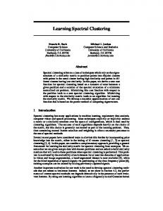
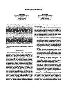
To illustrate the advantage of the proposed incremental eigenpair computation method, we compare the computation time between the proposed incremental method and the batch method both for varying K and varying graph size. The Erdos-Renyi random graphs that we build are used for this comparison. Fig. 1 (a) shows the computation time of incremental and batch computation methods for sequentially computing from K = 2 to K = 10 smallest eigenpairs. Fig. 1 (b) shows the computation time of both methods with respect to different graph size n. It is observed that the difference in computation time grows exponentially as n increases, which suggests that the proposed incremental method is more efficient than the batch computation method, especially for large graphs. 6.2 Clustering metrics for user-guided spectral clustering In real-life, an analyst can use the proposed incremental method along with a mechanism for selecting the best choice of K starting from K = 2. To demonstrate this, in the experiment we use five clustering metrics that can be used for online decision making regarding the value of K. These metrics are commonly used in

K=10

n=10000 400

batch computation method incremental computation method

350

computation time (seconds)

computation time (seconds)

400

300 250 200 150 100 50 0

0

2

4

6

8

number of eigenpairs K

(a)

10

12

batch computation method incremental computation method

350 300 250 200 150 100 50 0

0

2000

4000

6000

8000

10000

12000

number of nodes n

(b)

Figure 1: Sequential eigenpair computation time on Erdos-Renyi random graphs with edge connection probability p = 0.1. The markers are averaged computation time of 50 trials and the error bar represents standard deviation. (a) Computation time with n = 10000 and different number of eigenpairs K. (b) Computation time with K = 10 and different number of nodes n.

These metrics provide alternatives for gauging the quality of the clustering method. For example, Mod and NC reflect the trade-off between intracluster similarity and intercluster separation. Therefore, the larger the value of Mod, the better the clustering quality, and the smaller the value of NC, the better the clustering quality. Scaled spectrum energy is a typical measure of cluster quality for spectral clustering [15, 19, 28], and smaller spectrum energy means better separability of clusters. For Mod and scaled NC, a user might look for a cluster count K such that the increment in the clustering metric is not significant, i.e., the clustering metric is saturated beyond such a K. For scaled median and maximum cluster size, a user might require the cluster count K be such that the clustering metric is below a desired value. For scaled spectrum energy, a user might look for a noticeable increase in the clustering metric between consecutive values of K.

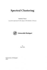
clustering unweighted and weighted graphs and they are summarized as follows. 1. Modularity: modularity is a widely used measure 6.3 Demonstration Here we use Minnesota Road data to demonstrate of clustering quality. how users can utilize the clustering metrics in Sec. 2   K  X W (Ci , Ci ) W (Ci , V) 6.2 to determine the number of clusters. The five Mod = (6.8) , − metrics evaluated for Minnesota Road clustering with W (V, V) W (V, V) i=1 respect to different cluster counts K are displayed in where V is the set of all nodes in the graph, Ci is the Fig. 2. Starting from K = 2 clusters, these metrics i-th cluster, W (Ci , Ci ) denotes the sum of weights of are updated by the incremental user-guided spectral all internal edges of the i-th cluster, W (Ci , Ci ) denotes clustering algorithm (Algorithm 1) as K increases. the sum of all external edge weights of the i-th cluster, If the user imposes that the maximum cluster size W (Ci , V) = W (Ci , Ci ) + W (Ci , Ci ), and W (V, V) = should be less than 30% of the total number of nodes, P n then the algorithm returns clustering results with a j=1 sj = s denotes the total nodal strength. 2. Scaled normalized cut: normalized cut (NC) is number of clusters of K = 6 or greater. Inspecting the defined as [27] modularity one sees it saturates at K = 7, and the user also observes a noticeable increase in scaled spectrum K X W (Ci , Ci ) energy when K = 7. Therefore, the algorithm can be NC = (6.9) . used to incrementally generate four clustering results W (C , V) i i=1 for K = 7, 8, 9, and 10. The selected clustering results Scaled normalized cut is NC divided by the number of in Fig. 3 are shown to be consistent with geographic clusters, i.e., NC/K. separations of different granularity. 3. Scaled median (or maximum) cluster size: We also apply the proposed incremental algorithm Scaled medium (maximum) cluster size is the medium for user-guided spectral clustering (Algorithm 1) to (maximum) cluster size of K clusters divided by the Power Grid, CLUTO, Swiss Roll, Youtube, and Blogtotal number of nodes n of a graph. Catalog. In Fig.5, we show how the value of cluster4. Scaled spectrum energy: scaled spectrum energy ing metrics changes with K, for each dataset. The inis the sum of the K smallest eigenvalues of the graph cremental method enables us to efficiently generate all Laplacian matrix L divided by the sum of all eigenvalues clustering results with K = 2, 3, 4 . . . and so on. Due to of L, which can be computed by space limitation, for each dataset we only show the trend PK of the three clustering metrics that exhibit the highest λi (L) variation for different K; thus, the chosen clustering (6.10) , scaled spectrum energy = Pi=1 n j=1 Ljj metrics can be different for different datasets. This suggests that selecting the correct number of clusters is a where λi (L) P is the i-th smallest eigenvalue of L and P difficult task and a user might need to use different clusn n j=1 Ljj = i=1 λi (L) is the sum of diagonal elements tering metrics for a range of K values. The proposed of L.

modularity 1 0.5 0

2

3

4

5

6

7

8

9

10

7

8

9

10

8

9

10

8

9

10

8

9

10

NC/K 0.04 0.02 0

2

3

4

5

6

median cluster size/n 0.5 0

2

3

4

5

6

7

(a) K = 7

(b) K = 8

(c) K = 9

(d) K = 10

maximum cluster size/n 1 0.5 0

2

3

4

1 0.5 0

2

5

6

7

scaled spectrum energy

−5

x 10

3

4

5

6

7

K

Figure 2: Five clustering metrics computed incrementally via Algorithm 1 for Minnesota Road.

7

Figure 3: Visualization of user-guided spectral clustering on Minnesota Road with respect to selected cluster count K. Colors represent different clusters. 2.5

log(1 + Batch Time - Incremental Time)

incremental eigenpair computation is an effective tool to support such an endeavor. In addition, Fig. 4 shows the time improvement of the proposed incremental method relative to the batch method, where the difference in computation time is displayed in log scale to accommodate large variance of time improvement across datasets that are of widely varying size. It is observed that the gain in computational time via the proposed incremental method is more pronounced as cluster count increases, which demonstrates the merit of the proposed method. Theorem 3.1 establishes that the proposed incremental method exactly computes the K-th eigenpair using 1 to (K − 1)-th eigenpairs, yet for the sake of experiments with real dataset, we have computed the normed eigenvalue difference and eigenvector correlation of the K smallest eigenpairs using the batch method and the proposed incremental method. The K smallest eigenpairs are identical as expected; to be specific, using Matlab library, on the Minnesota road dataset for K = 20, the normed eigenvalue difference is 7 × 10−12 and the associated eigenvectors are identical up to differences in sign. Results for the other datasets are available in the supplementary file.

2.0

Cluster Count = 5 Cluster Count = 10 Cluster Count = 15 Cluster Count = 20

1.5

1.0

0.5

0.0

oad Grid sota R Power Minne

CLUTO

Roll Swiss

be Youtu

atalog BlogC

Figure 4: Computation time improvement of the proposed incremental method relative to the batch method. increases. We demonstrate that the proposed incremental eigenpair computation method is an effective tool for a user-guided spectral clustering task, which effectively updates clustering results and metrics for each increment of the cluster count.

Conclusion

This paper establishes an efficient incremental eigen- References pair computation method for graph Laplacian matrices by transforming a batch eigenvalue decomposition [1] S. Basu, A. Banerjee, and R. J. Mooney. Active problem into a sequential leading eigenpair computasemi-supervision for pairwise constrained clustering. In tion problem. The proposed method achieves signifSDM, volume 4, pages 333–344, 2004. icant reduction in computation time when compared [2] M. Belkin and P. Niyogi. Laplacian eigenmaps for diwith the batch computation method. Particularly, it mensionality reduction and data representation. Neuis observed that the difference in computation time of ral computation, 15(6):1373–1396, 2003. these two methods grows exponentially as the graph size [3] P.-Y. Chen and A. Hero. Deep community detection.

modularity

modularity

modularity

1

1

1

0.5

0.5

0.5

0

2

4

6

8

10

12

14

16

median cluster size/n

18

20

0.5

0

2

4

6

8

10

12

14

16

maximum cluster size/n

18

20

1

0

modularity

modularity

0.5

0.2 0

2

4

6

8

10

12

14

16

18

median cluster size/n

20

0.5

0

2

4

6

8

10

12

NC/K

14

16

18

20

0.2

0.5

−0.2

2

4

2

4

2

4

6

8

10

12

14

16

18

20

6

8

10

12

14

16

18

20

6

8

10

12

14

16

18

20

NC/K

1 0.8

0.1

0.6 0

2

4 −5

1

x 10

6

8

10

12

14

16

scaled spectrum energy

18

20

0

2

4 −4

2

0.5

x 10

6

8

10

12

14

16

scaled spectrum energy

18

20

0

2

4 −6

2

1

x 10

6

8

10

12

14

16

18

scaled spectrum energy

20

0

2

4

6

8

10

12

14

16

maximum cluster size/n

18

20

1

1

maximum cluster size/n

1

0.8

0.5

0.6 0

2

4

6

8

10

12

14

16

18

K

(a) Power Grid

20

0

2

4

6

8

10

12

14

16

18

20

0

2

4

6

8

K

(b) CLUTO

10

12

14

16

18

K

20

2

4

6

8

10

12

14

16

K

(c) Swiss Roll

(d) Youtube

18

20

0

K

(e) BlogCatalog

Figure 5: Three selected clustering metrics of each dataset. The complete clustering metrics can be found in the supplementary file.

[4]

[5]

[6]

[7]

[8] [9]

[10]

[11]

[12]

[13] [14]

[15]

[16]

[17]

IEEE Trans. Signal Process., 63(21):5706–5719, Nov. 2015. P.-Y. Chen and A. Hero. Phase transitions in spectral community detection. IEEE Trans. Signal Process., 63(16):4339–4347, Aug 2015. P.-Y. Chen and A. O. Hero. Node removal vulnerability of the largest component of a network. In GlobalSIP, pages 587–590, 2013. P.-Y. Chen and A. O. Hero. Assessing and safeguarding network resilience to nodal attacks. IEEE Commun. Mag., 52(11):138–143, Nov. 2014. C. Dhanjal, R. Gaudel, and S. Cl´emen¸con. Efficient eigen-updating for spectral graph clustering. Neurocomputing, 131:440–452, 2014. R. A. Horn and C. R. Johnson. Matrix Analysis. Cambridge University Press, 1990. P. Jia, J. Yin, X. Huang, and D. Hu. Incremental laplacian eigenmaps by preserving adjacent information between data points. Pattern Recognition Letters, 30(16):1457–1463, 2009. J. Kuczynski and H. Wozniakowski. Estimating the largest eigenvalue by the power and lanczos algorithms with a random start. SIAM journal on matrix analysis and applications, 13(4):1094–1122, 1992. C. Lanczos. An iteration method for the solution of the eigenvalue problem of linear differential and integral operators. Journal of Research of the National Bureau of Standards, 45(4), 1950. R. B. Lehoucq, D. C. Sorensen, and C. Yang. ARPACK users’ guide: solution of large-scale eigenvalue problems with implicitly restarted Arnoldi methods, volume 6. Siam, 1998. U. Luxburg. A tutorial on spectral clustering. Statistics and Computing, 17(4):395–416, Dec. 2007. R. Merris. Laplacian matrices of graphs: a survey. Linear Algebra and its Applications, 197-198:143–176, 1994. A. Y. Ng, M. I. Jordan, and Y. Weiss. On spectral clustering: Analysis and an algorithm. In NIPS, pages 849–856, 2002. H. Ning, W. Xu, Y. Chi, Y. Gong, and T. S. Huang. Incremental spectral clustering with application to monitoring of evolving blog communities. In SDM, pages 261–272, 2007. H. Ning, W. Xu, Y. Chi, Y. Gong, and T. S. Huang. Incremental spectral clustering by efficiently updating

[18]

[19] [20]

[21]

[22]

[23]

[24]

[25]

[26]

[27]

[28] [29]

the eigen-system. Pattern Recognition, 43(1):113–127, 2010. R. Olfati-Saber, J. Fax, and R. Murray. Consensus and cooperation in networked multi-agent systems. Proc. IEEE, 95(1):215–233, 2007. M. Polito and P. Perona. Grouping and dimensionality reduction by locally linear embedding. In NIPS, 2001. L. K. M. Poon, A. H. Liu, T. Liu, and N. L. Zhang. A model-based approach to rounding in spectral clustering. In UAI, pages 68–694, 2012. A. Pothen, H. D. Simon, and K.-P. Liou. Partitioning sparse matrices with eigenvectors of graphs. SIAM journal on matrix analysis and applications, 11(3):430– 452, 1990. F. Radicchi and A. Arenas. Abrupt transition in the structural formation of interconnected networks. Nature Physics, 9(11):717–720, Nov. 2013. G. Ranjan, Z.-L. Zhang, and D. Boley. Incremental computation of pseudo-inverse of laplacian. In Combinatorial Optimization and Applications, pages 729–749. Springer, 2014. J. Shi and J. Malik. Normalized cuts and image segmentation. IEEE Trans. Pattern Anal. Mach. Intell., 22(8):888–905, 2000. D. Shuman, S. Narang, P. Frossard, A. Ortega, and P. Vandergheynst. The emerging field of signal processing on graphs: Extending high-dimensional data analysis to networks and other irregular domains. IEEE Signal Process. Mag., 30(3):83–98, 2013. S. White and P. Smyth. A spectral clustering approach to finding communities in graph. In SDM, volume 5, pages 76–84, 2005. M. J. Zaki and W. M. Jr. Data Mining and Analysis: Fundamental Concepts and Algorithms. Cambridge University Press, 2014. L. Zelnik-Manor and P. Perona. Self-tuning spectral clustering. In NIPS, pages 1601–1608, 2004. B. Zhang, T. K. Saha, and M. A. Hasan. Name disambiguation from link data in a collaboration graph. In ASONAM, pages 81–84, 2014.

Supplementary File 8 Appendix 8.1 Proof of Lemma 3.2 Lemma 8.1. Assume that G is a disconnected P graph with δ ≥ 2 connected components, and let s = ni=1 si , e = L+ let V = [v1 (L), v2 (L), . . . , vδ (L)], and let L T e vi (L)) e = (λi+δ (L), vi+δ (L)) for sVV . Then (λi (L), e 1 ≤ i ≤ n − δ, λi (L) = s for n − δ + 1 ≤ i ≤ n, and e vn−δ+2 , (L), e . . . , vn (L)] e = V. [vn−δ+1 (L),

Theorem 8.1. (disconnected graphs) Assume that G is a disconnected graph with δ ≥ 2 connected components, given VK,δ , ΛK,δ and K ≥ δ, the eigenpair (λK+1 (L), vK+1 (L)) is a leading eigenpair e = L + VK,δ ΛK,δ VT + sVδ VT − sI. of the matrix L K,δ δ In particular, if L has distinct nonzero eigenvalues, then e + s, v1 (L)). e (λK+1 (L), vK+1 (L)) = (λ1 (L)

Proof. First observe from (8.11) that L has δ zero eigenvalues since each connected component contributes to exactly one zero eigenvalue for L. Following the same derivation procedure in the proof of Theorem 3.1 and Proof. The graph Laplacian matrix of a disconnected using Lemma 3.2, we have graph can be represented as a component-wise union T e = L + VK,δ ΛK,δ VK,δ + sVδ VδT − sI L of δ graph Laplacian matrices corresponding to each n X connected component [5], i.e., (8.13) = (λi (L) − s)vi (L)viT (L).   i=K+1,K≥δ L1 O O O  O L2 O O  Therefore, the eigenpair (λK+1 (L), vK+1 (L)) can be   (8.11) L= , . e If . obtained by computing the leading eigenpair of L. O O . O L has distinct nonzero eigenvalues (i.e, λδ+1 (L) < O O O Lδ λδ+2 (L) < . . . < λn (L)), we obtain the relation e + s, v1 (L)). e where Lk is the graph Laplacian matrix of k-th con- (λK+1 (L), vK+1 (L)) = (λ1 (L) nected component in G. From the proof of Lemma 3.1 each connected component contributes to exactly one 8.4 Complete clustering metrics for userguided spectral clustering zero eigenvalue for L, and Fig. 6 displays the five clustering metrics introduced in δ X X Sec. 6.2 on Power Grid, CLUTO, Swiss Roll, Youtube, λn (L) < λi (Lk ) and BlogCatalog. These metrics are computed increk=1 i∈component k mentally via Algorithm 1 and they provide multiple δ criterions for users to decide the final cluster count. For X X = si instance, for Swill Roll if an user decides to stop at k=1 i∈component k K = 8 clusters, the selected clustering results are shown in Fig. 5. It is observed that the selected clustering re(8.12) = s. sults indeed yield satisfactory outcomes that separate the data points according to their geodesic distances on Therefore, we have the results in Lemma 3.2. the two-dimensional manifold. 8.2 Proof of Corollary 3.2 8.5 Demonstration of equivalence between the Corollary 8.1. For a normalized graph Lapla- proposed incremental computation method and cian matrix LN , assume G is a disconnected the batch computation method graph with δ ≥ 2 connected components. Let Here we use the K smallest eigenpairs of the datasets Vδ = [v1 (LN ), v2 (LN ), . . . , vδ (LN )], and let in Table 2 computed by the batch method and the e N = LN + 2Vδ VT . Then (λi (L e N ), vi (L e N )) = proposed incremental method to verify Theorem 3.1, L δ (λi+δ (LN ), vi+δ (LN )) for 1 ≤ i ≤ n − δ, which proves that the proposed incremental method exe N ) = 2 for n − δ + 1 ≤ i ≤ n, and actly computes the K-th eigenpair using 1 to (K − 1)-th λi (L e N ), vn−δ+2 , (L e N ), . . . , vn (L e N )] = Vδ . eigenpairs. Fig. 6 shows the normed eigenvalue differ[vn−δ+1 (L ences and the correlations of the associated eigenvectors Proof. The results can be obtained by following the obtained from the two methods. It can be observed that same derivation procedure in Appendix 8.1 and the fact the normed eigenvalue difference is negligible and the associated eigenvectors are identical up to the difference that λn (LN ) ≤ 2 [14]. in sign, i.e., the eigenvector correlation in magnitude equals to 1 for every eigenvector of the two methods. 8.3 Proof of Theorem 3.2

modularity 1 0.5 0

2

4

6

8

10

12

14

16

18

20

14

16

18

20

16

18

20

14

16

18

20

14

16

18

20

14

16

18

20

14

16

18

20

16

18

20

14

16

18

20

14

16

18

20

NC/K 0.04 0.02 0

2

4

6

8

10

12

median cluster size/n 0.5 0

2

4

6

8

10

12

14

maximum cluster size/n 1 0.5 0

2

4

6

8

1 0.5 0

2

10

12

spectrum energy

−5

x 10

4

6

8

10

12

K (a) Power Grid

modularity 1 0.5 0

2

4

6

8

10

12

NC/K 0.1 0.05 0

2

4

6

8

10

12

median cluster size/n 0.5 0

2

4

6

8

10

12

14

maximum cluster size/n 1 0.5 0

2

4

6

8

2 1 0

x 10

2

10

12

spectrum energy

−4

4

6

8

10

12

K (b) CLUTO

Figure 6: Multiple clustering metrics of different datasets. The metrics are modularity, scaled normalized cut (NC/K), scaled median and maximum cluster size, and scaled spectrum energy.

modularity 1 0.5 0

2

4

6

8

10

12

14

16

18

20

14

16

18

20

16

18

20

14

16

18

20

14

16

18

20

NC/K 0.04 0.02 0

2

4

6

8

10

12

median cluster size/n 0.5 0

2

4

6

8

10

12

14

maximum cluster size/n 1 0.5 0

2

4

6

8

2 1 0

2

10

12

spectrum energy

−6

x 10

4

6

8

10

12

K (c) Swiss Roll

modularity 0.5 0

2

4

6

8

10

12

14

16

18

20

14

16

18

20

16

18

20

14

16

18

20

14

16

18

20

NC/K 0.2 0.1 0

2

4

6

8

10

12

median cluster size/n 0.5 0

2

4

6

8

10

12

14

maximum cluster size/n 1 0.8 0.6 2

4

6

8

5 0

2

10

12

spectrum energy

−5

x 10

4

6

8

10

12

K (d) Youtube

modularity 0.2 0 −0.2

2

4

6

8

10

12

14

16

18

20

14

16

18

20

16

18

20

14

16

18

20

14

16

18

20

NC/K 1 0.8 0.6 2

4

6

8

10

12

median cluster size/n 0.5 0

2

4

6

8

10

12

14

maximum cluster size/n 1 0.5 0

2

4

6

8

1 0.5 0

2

10

12

spectrum energy

−4

x 10

4

6

8

10

12

K (a) BlogCatalog

20 10 0 −10 −20 15

50 10

5

0

−5

−10

−15

0

10

5

0

−5

−10

−15

0

20 10 0 −10 −20 15

50

Figure 5: Visualization of user-guided spectral clustering on Swiss Roll with K = 8 clusters. Spectral clustering is performed on the two-dimensional embedding dataset4 that preserves geodesic distances among data points of the original dataset. Top: the original data. Bottom: clustering results. Colors represent different clusters.

x 10

normed eigenvalue difference

normed eigenvalue difference

−12

8 6 4 2 0

5

10

15

20

−11

8

x 10

6 4 2 0

5

number of smallest eigenpairs K

1 0.5

0

5

10

15

20

0.5 0

25

0

5

x 10

3 2 1 5

10

15

20

x 10

8 6 4 2 0

5

10

15

20

1.5

correlation magnitude

correlation magnitude

25

number of smallest eigenpairs K

1.5 1 0.5

0

5

10

15

20

1 0.5 0

25

0

5

smallest eigenpairs

normed eigenvalue difference

x 10

3 2 1 0

5

10

15

20

25

20

−11

1

x 10

0.5

0

5

number of smallest eigenpairs K

10

15

20

number of smallest eigenpairs K 1.5

correlation magnitude

1.5 1 0.5 0

15

(d) Swiss Roll

−10

4

10

smallest eigenpairs

(c) CLUTO normed eigenvalue difference

20

(b) Power Grid

number of smallest eigenpairs K

correlation magnitude

15

−11

normed eigenvalue difference

normed eigenvalue difference

(a) Minnesota Road

0

10

smallest eigenpairs

−11

0

20

1

smallest eigenpairs

4

15

1.5

correlation magnitude

correlation magnitude

1.5

0

10

number of smallest eigenpairs K

0

5

10

15

smallest eigenpairs

(e) Youtube

20

25

1 0.5 0

0

5

10

15

20

25

smallest eigenpairs

(f) BlogCatalog

Figure 6: Comparisons of the smallest eigenpairs by the batch method and the proposed incremental method for datasets listed in Table 2.

modularity 1 0.5 0

2

4

6

8

10

12

14

16

18

20

14

16

18

20

16

18

20

14

16

18

20

14

16

18

20

NC/K 0.05 0

2

4

6

8

10

12

median cluster size/n 0.5 0

2

4

6

8

10

12

14

maximum cluster size/n 1 0.5 0

2

4

6

8

4 2 0

x 10

2

10

12

spectrum energy

−5

4

6

8

10

12

K

normed eigvalue difference

−12

8

x 10

6 4 2 0

5

10

15

20

number of smallest eigenpairs K correlation maganitude

1.5 1 0.5 0

0

5

10

15

smallest eigenpairs

20

25