Indoor Localization by Denoising Autoencoders and Semi-supervised ...

Indoor Localization by Denoising Autoencoders and Semi-supervised Learning in 3D Simulated Environment Amirhossein Shantia∗ , Rik Timmers∗ , Lambert Schomaker∗ , Marco Wiering∗ ∗ Institute

of Artificial Intelligence and Cognitive Engineering University of Groningen, Groningen, The Netherlands a.shantia, r.p.timmers, l.r.b.schomaker, [email protected]

Abstract—Robotic mapping and localization methods are mostly dominated by using a combination of spatial alignment of sensory inputs, loop closure detection, and a global fine-tuning step. This requires either expensive depth sensing systems, or fast computational hardware at run-time to produce a 2D or 3D map of the environment. In a similar context, deep neural networks are used extensively in scene recognition applications, but are not yet applied to localization and mapping problems. In this paper, we adopt a novel approach by using denoising autoencoders and image information for tackling robot localization problems. We use semi-supervised learning with location values that are provided by traditional mapping methods. After training, our method requires much less run-time computations, and therefore can perform real-time localization on normal processing units. We compare the effects of different feature vectors such as plain images, the scale invariant feature transform and histograms of oriented gradients on the localization precision. The best system can localize with an average positional error of ten centimeters and an angular error of four degrees in 3D simulation.

I.

I NTRODUCTION

The commercial availability of robots is currently limited to small service robots such as vacuum cleaners, lawn mowers, and experimental robots for developers. Recently, however, there is a clear rise of consumer interest in home robotics. One example is the development of service robots that operate in home and office environments. These robots must be priced congruent with their abilities. In this paper, we join the current trend of focusing more on smart software solutions combined with low-cost hardware requirements to facilitate the process of creating cheaper robots with reliable functionalities. With this goal in mind, we focus on a very basic functionality of a sophisticated robot, localization. Currently, the most well-known and commonly used approaches for solving the localization problem are through a precise process of mapping the environment using 2D or 3D sensory data and their required algorithms. These recursive and incremental updating methods generally consist of three major parts, spatial alignment of data frames, loop closure detection, and a global fine-tuning step [1], [2]. The hardware requirements for these methods, however, can be quite expensive. For example, the cheapest 2D laser range finder roughly costs hundreds of Euros, and the price exponentially increases when more precision and robustness are added to the sensor. There has been valuable research done on this topic in the recent years, especially by using the fairly inexpensive

Primesense sensor 1 found on Microsoft Kinect devices. Henry et al [4], introduced a 3D indoor mapping method using a combination of RGB feature-based methods and depth images to connect the frames and close the loops. The results of this work are a very good approximation of challenging environments visualized in a 3D map. The calculations however, took approximately half a second per frame to compute. Whelan et al [5], on the other hand, promised a real time delivery of mapping and localization by the use of high performance GPUs and expensive hardware. Another issue that has not yet been addressed with these methods is the effect of luminance from outside sources to the process of mapping. In [6], the authors mention that the lighting condition influences the correlation and measurement of disparities. The laser speckles appear in low contrast in the infrared image in the presence of strong light. Sun light through windows, behind a cloud, or its reflection off the walls and the floor can introduce non-existing pixel patches or gaps to the depth image. Therefore, additional research is required to measure these effects, and perhaps to introduce new methods that require less computational power at run-time which are robust to external sources and changes to the environment. In a similar context, there has been significant research on image classification and scene recognition using deep neural networks in the recent years [7]–[10]. This has allowed the community to achieve high classification performance in character, scene and object recognition challenges [11]–[13]. In this paper, we adopt a novel approach to the localization problem by using denoising autoencoders (DA) [14] with HSV color-space information. We use a semi-supervised approach to learn the location values provided by traditional mapping and localization methods such as Adaptive Monte Carlo localization (AMCL), and Grid Mapping [2], [15]. This approach has a significant run-time advantage over the traditional ones due to the low computational requirement of a feed-forward neural network. It is only the initial training of the network that requires a significant amount of computation which can be done offline and delegated to other sources such as cloud computing centers (e.g. Amazon Web Services). Another benefit is the general ability of neural networks to cope with sensor noise. We combine multiple feature vectors with the DA and compare them to other scene recognition 1 Primesense

Ltd. Patent No.US7433024 [3]

methods such as histograms of oriented gradients (HoG) [16]. In a commercial scenario, the manufacturer can temporarily install a depth sensor during the product delivery/installation and perform a traditional mapping to record the approximate ground truth for each captured image. The robot will then start the training of the (deep) neural network, and the depth sensor can be removed. Finally, the robot can continue localizing with acceptable error rate. In short, our method: •

is a novel approach for localization using denoising autoencoders with semi-supervised learning

•

has low run-time computation requirements

•

has inexpensive hardware requirements

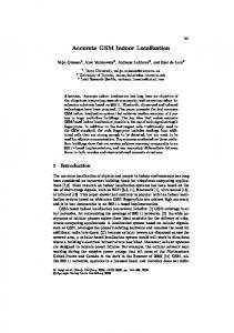
A. Feature sets Indoor localization requirements are slightly different compared to those for normal scene recognition where the goal is to distinguish totally different types of scenes from each other. For example, in the SUN [17] and indoor CVPR [13] databases, there are different types of scenes such as offices, trees, zoos, etc. In each of these classes the details in the scenery are different, but they share a set of similar objects or landscapes (Figure 2). For robot navigation in indoor environments, however, the robot needs to distinguish similar scenes with different scale and rotation from each other. In some cases (Figure 3), moving forward for a couple of meters does not change the scenery, or there are views that look the same, but are in fact, taken from different locations. In order to select a good feature set, we use some established feature vectors and carry out the experiments using them.

We also compare the effect of different feature vectors on localization precision and conclude that the positional and angular errors can compete with those of traditional methods. In section II, we explain the features, the neural networks, and the training methods in detail. We discuss our experimental setup and the obtained results in section III. We finally conclude the paper in section IV and discuss future work in section V. II.

M ETHODOLOGY

In this section we first discuss the different feature vectors used for training with denoising autoencoders (DA), and the reasons for selecting them for localization purposes. Next, we continue with an explanation of the pre-training of the DA network, and a second layer neural network that is used for learning the metric location values. A block diagram of the complete pipeline is depicted in Figure 1.

Fig. 2. Samples from the ICVPR dataset. The office environments share the same characteristics, but are totally different from one another.

Image & Position Storage

Image Resizing

SDA Training

Localization Network Training

Location Estimating

Fig. 1. The block diagram of required steps for training and testing the proposed approach.

Fig. 3. Sample images from our robotics laboratory. The pictures taken show the same scenery, but the robot was positioned in different locations.

1) Sub-sampled Plain Image: The original raw image contains a lot of information about the scene. Due to the large size of images, applying machine learning techniques becomes difficult on the basis of the curse of dimensionality [18]. However, it is possible to extract a sub-sample of the original image, which results in a much smaller feature vector. The downside of this method is that we may lose fine-grained cues that are present in the original image. Krizhevsky et al. in [9], and [19], demonstrated the learning ability of deep neural networks using plain images. In [9], the authors used a combination of convolutional neural networks (CNN) [20] and traditional neural networks to solve a one thousand class problem with more than a million training images [12]. In [19],

the authors used a very deep autoencoder with plain images to retrieve a set of images from the CIFAR [11] database. Since their experiments showed promising results using only plain images, we also use a sub-sampled plain image in our feature set. On this basis, we use a flattened gray-scale and HSV colorspace image with a fixed size of 28 × 28. We perform the resampling using pixel area relation, which is a preferred method for image decimation. This results in 784 input dimensions for the gray scale image and 2352 input dimensions for the HSV image. The HSV coloring system is preferred to RGB because of its resistance to lighting changes. We will use the subsampled plain image feature as a baseline for our comparisons. 2) Sub-sampled image with top SIFT keypoints: On the one hand, sampling down the camera image has the advantage of retaining the scene structure, and also reducing noise. It also allows the system to cope better with color and light variations. On the other hand, it has a disadvantage of losing fine, high resolution sections of the image which can be essential in detailed scene recognition and localization. For example, a key switch in the kitchen, or a prominent door handle can give hints to the robot about its actual location. In order to scale down this effect, we decided to use a combination of sub-sampled plain images, and prominent SIFT features [21] extracted from each image. For each image, we calculate the SIFT features for the original high-resolution image. The top four keypoints are selected from each image based on their SIFT response value, and their descriptors are added to the plain image feature set. This approach may help the system to retain prominent image structures while learning from general information of the sub-sampled image. 3) Histograms of Oriented Gradients: We decided to use yet another method while bypassing the autoencoder to compare the performance with the other two proposed methods. We used the idea of histograms of oriented gradients which was previously applied to human detection [16], and for indoor localization [22]. We, however, decided to calculate the HoG of additional blocks with varying sizes to capture both general and detailed edge information of the scene using the spatial pyramids approach [23]. The image is divided into separate blocks of 8 × 8, 4 × 4, and 2 × 2. The gradients for all of the blocks and the image itself are then calculated. This results in 680 values for the feature vector.

Then, the corrupted input is fed through a matrix product with the first layer of weights, and the bias vector is added to the hidden layer neuron activations. Finally the results go through a sigmoid function (eq. 2):

y = fθ (˜ x) = ς(W˜ x + b)

In the next step, the network attempts to reconstruct the original input vector (eq. 3): z = gθ0 (y) = ς(W0 y + b0 )

(3)

The cost function used is the reconstruction cross-entropy depicted in equation 4:

L(x, z) = −

d X

[xk log zk + (1 − xk ) log(1 − zk )]

(4)

k=1

In which x is the original input which is normalized between 0 and 1, z is the reconstructed output from the corrupted input, and k denotes the index of the input vector. By using this equation, the error and the updates of one stochastic gradient descent can be calculated. After sufficient epochs, the training of the first layer is stopped. Figure 4(a) shows this process. y

LH(x,z)

Fϴ

Gϴ

qD x

z

(a) y

LH(x,z)

Fϴ(2)

Gϴ

qD z Fϴ

B. Denoising Autoencoder Training

x

We decided to perform indoor scenery recognition using the denoising autoencoder [14] because of the simplicity of the training procedure compared to convolutional neural networks. Stacked formation of denoising autoencoders (DAs) and their strong learning ability and low error rate compared to support vector machines, the restricted Boltzmann machine (RBM), and traditional autoencoders [8], [14], [24], are other reasons for selecting this approach. 1) Pre-training: Pre-training under the influence of noise is the part that distinguishes a denoising autoencoder from a traditional autoencoder. The input of the network is corrupted by either random masking, salt and pepper, or Gaussian noise, etc. (eq. 1): x→ − x ˜ ∼ qD (˜ x|x)

(2)

(1)

(b) Fig. 4. The input x is corrupted using the qD function. Then the result is fed forward to the next layer using the fθ of equation 2. Afterwards, a reconstruction attempt to the original input is made using the gθ of equation 3. Finally the error at the outputs are backpropagated through the neural network. For the stacked version, the non-corrupted input is fed forward up to level n of the network before applying the corruption.

The training of a stacked denoising autoencoder (SDA) is similar to that of a DA, but with a small difference in the higher layers. Consider that the network is trained up to layer n − 1, and we want to train the final layer n. For input x, output fθ of the layer n − 1 is extracted using traditional feedforward neural network algorithms. Then, this output vector is corrupted using qD (˜ x|x), and after that the output of the

nth layer is calculated. An attempt is made to reconstruct the original nth layer output using the corrupted nth layer input (Figure 4(b)). The type, and amount of the corruption has a large effect on the result of pre-training. Parameters used in our experiments will be discussed further in section III. 2) Semi-supervised Location Estimation using Ground Truth: In order to associate the ground truth location values to the encoded result of the neural network, we connect a secondary two layer feedforward neural network to the learned encoding of the input. In our experiments, we record the ground truth data using the perfect robot odometry in 3D simulation. The relation between the scenes and the odometry readings is a non-linear function, and we can learn this by using a feedforward neural network with non-linear activation functions. In order to achieve this goal, the following procedure is followed. After the pre-training phase of the SDA is completed, we add a separate neural network with one hidden layer on top of the denoising autoencoder. The hidden layer activation function is a sigmoid, and the output layer has a linear activation. The outputs of the neural network consist of normalized metric X and Y values, and the sin(θ) and cos(θ) with θ being the robot angle in radians. Reasons for selecting sine and cosine of the radian are that first the values are bounded and between [−1, 1], and can be easily normalized to [0, 1], and we want to give a hint to the neural network that the angular input is not continuous, but has a periodic property. The network can learn this by observing the 3rd and 4th output. The normalization factors of X and Y come from the ground truth map available through the simulation. Fine-tuning layers in classification problems such as in [9], [14], [19], have a one layer network where their outputs were either the class label or the softmax probability of each class. Our problem, however, is of the regression type, and a hidden layer is required to non-linearly map the encoded outputs to the position and angular values. In addition, in those papers, the class labels are used to further reduce the reconstruction error of the network. In our case, however, we merely aim at associating location values to the encoded outputs. Therefore, we do not propagate the error through the whole network. Consequently, using the mean squared error as our error function, the back propagation rule is used to train the weights of the location estimating neural network. III.

E XPERIMENTS

We carried out our experiments using the Gazebo (v3.0) 3D physics simulator [25], and used the ROS framework to develop our software [26]. We used Gazebo with the Bullet 3D physics engine which allows for the use of GPUs to facilitate a real-time simulation and high frame rates for all the robot sensory inputs using an ordinary PC. The environment used for the experiments can be seen in Figure 52 . We used FANN, OpenCV, and Theano libraries to perform the SDA, and location estimation neural network training phases, [27], [28], [29]. Theano uses multiple cores and a GPU to perform the SDA training steps. 2 https://3dwarehouse.sketchup.com.

Fig. 5. The 3D model of the environment. The model is a modified version of the Cherry Kitchen model in Google’s 3D warehouse.

The simulated robot, which can be seen in Figure 6 is used for our experiments. The robot consists of a moving base with differential drive, and a top frame which carries its essential depth and RGB sensors, a laser range finder, manipulator and an interface for human robot interaction. We modeled our laboratory robot in Gazebo using the Unified Robot Description Format (URDF), which is an XML format for representing a robot model. The model shapes and meshes used in simulation were partly generated by the vendors and partly designed by ourselves.

Fig. 6.

3D model of the robot used for the experiments.

All the neural network training simulations are repeated 10 times with different initializations of the neural networks. The baseline, which is the sub-sample plain image, is not given to the SDA for high level feature extraction. The HoG features are also not processed by the SDA because these features are already a representation/compression of the full image. After the autoencoder training is finished, training of the location estimation neural network starts. We only update the weights of the location estimation neural networks without propagating it back to the SDA network. We explored multiple network and training configurations in the 3D simulation and selected the best ones based on localization performance and computational requirements. We found out that the number of required neurons in each layer can be one third of the number of inputs. The results would increase slightly if the number of neurons increases. However, the speed of calculation decreases during training and prediction phases which is not suitable for a real-time robot. Therefore, we decided to limit the number of neurons as much as possible. The denoising autoencoder network with gray scale input images uses 256 hidden neurons, and the networks with HSV and HSV+SIFT input images use 750 hidden neurons per layer. For the sub-sampled plain image

with top SIFT keypoints, we kept the number of neurons in each layer the same to make sure the comparison is valid. The HoG feature vector, however, does not require the autoencoder so it is left out of this part of training. The learning rate for training the SDA was set to 0.001. The neural network used for estimating the location of the robot is a single hidden layer neural network with sigmoid functions in the hidden layer and a linear activation function in the output layer. There are hundred neurons in the hidden layer and four outputs which represent X, Y, sin(θ), cos(θ), respectively. Finally, for the sub-sampled plain image vectors, the encoding of the images are processed and then fed to the localizing neural network. The HoG feature vector is directly fed to the localizing neural network. The training of the localizing neural network is done by traditional back propagation with the learning rate of 0.001 and 10, 000 epochs with no stopping criteria. To prevent overfitting, we record the network every hundred epochs and only use the network with highest validation performance for the final experiment with the test dataset.

A. 3D Simulation The simulation environment is a kitchen with a dimension of 5 × 7 meters. It contains both detailed and coarse objects. The lighting is provided by a unified directional beam (simulated sun), and two additional light bulbs. Only walls and object shadows are visible, because the current texture properties of the environment do not include light reflection properties. The data gathering is done through automatic and manual processes to collect training, validation, and test data. In the automatic method, the robot takes random discrete actions. Before performing an action, the robot saves the current ground truth location by using odometry in simulation. It then starts to take pictures while rotating from minus to plus five degrees around that point. This is to make sure that the robot has similar training data for the approximate same location in the environment. The robot is equipped with an obstacle avoidance system, and will change trajectory if it is close to an obstacle. In order to make sure that all locations are traversed, we let the robot operate for several hours and take a data set with 150 thousand training pictures. These pictures are used to train the denoising autoencoder. For training the location estimation layer, we gather a more structured data set of 10 thousand training, and 2 thousand validation and testing pictures. A human operator controls the robot, and takes steps of 0.5−1.5 meter. After each step he/she will rotate the robot in a full circle to capture the surroundings. This operation is repeated until the environment is covered. Since the lighting effects are incomplete in the 3D simulation, we avoid taking pictures of only walls. One side of the kitchen has continuous walls with the same texture, and no lighting changes. We make sure that another part of the kitchen is also in the view. Otherwise, it would be impossible for the robot to correctly estimate its position. For the validation and testing set, however, the operator will move the robot in a path for which the overlap with the previous run is minimal.

B. Experimental Results We first discuss the results of different network architectures and training configurations. Next, we elaborate the final performance of these networks using the features mentioned in section II-A. We tested a 1 layer DA with gray scale images, and different SDA architectures (1-3 layers) with HSV images using multiple training epochs in 3D simulation. The binomial corruption levels were started at 0.1. For each additional layer, the corruption level was increased by 0.1. We selected the corruption levels similar to other applications of SDA for scene and character recognition in [14]. Tables I and II show that the HSV results are significantly superior in comparison to the gray-scale. The reason is that the HSV images contain more information about the scene. TABLE I. T HE AVERAGE POSITIONAL ( METERS ) ERROR FOR HSV FEATURE VECTORS WITH 1-3 DENOISING AUTOENCODER LAYERS VERSUS DIFFERENT TRAINING EPOCHS . W E ALSO INCLUDED THE GRAY SCALE IMAGE WITH A 1 LAYER DENOISING AUTOENCODER . T HE ONE LAYER NETWORK WITH HSV IMAGES IS THE BEST CONSIDERING COMPUTATIONAL REQUIREMENTS AND THE LOCALIZATION ERROR .

Networks HSV - 1 Layer HSV - 2 Layer HSV - 3 Layer Gray Scale

20 Epochs 0.165 0.155 0.240 0.410

40 Epochs 0.140 0.152 0.210 0.370

60 Epochs 0.150 0.151 0.210 0.351

TABLE II. T HE AVERAGE ANGULAR ( RADIAN ) ERROR FOR HSV FEATURE VECTORS WITH 1-3 DENOISING AUTOENCODER LAYERS VERSUS DIFFERENT TRAINING EPOCHS . W E ALSO INCLUDED THE GRAY SCALE IMAGE WITH A 1 LAYER DENOISING AUTOENCODER . T HE ONE LAYER NETWORK WITH HSV IMAGES IS THE BEST CONSIDERING COMPUTATIONAL REQUIREMENTS AND THE LOCALIZATION ERROR .

Networks HSV - 1 Layer HSV - 2 Layer HSV - 3 Layer Gray Scale

20 Epochs 0.07 0.08 0.11 0.19

40 Epochs 0.06 0.07 0.09 0.18

60 Epochs 0.05 0.07 0.09 0.16

The three layer HSV network performs worse in comparison to the two and one layer networks. It is possible that the type and amount of corruption is not suited for this number of layers in the SDA and our application. The two layer network performs slightly better using a smaller number of epochs, but the one layer DA network catches up when more training is done on the denoising network. However, computationally the one layer network is superior because it takes much less time to train the network. Since the positional and angular errors of two and one layer network are similar, we decided to select the one layer networks for the rest of the experiments. In addition to the localization results, a reconstruction attempt of the scenes is depicted in Figure 7. We compared the final location performance of all network configurations with their features. The sub-sampled plain HSV images which were not given to the DA networks, but immediately to the location estimation neural network, are now selected as our baseline. The HoG features were also directly connected to the location estimating feedforward neural network. The HSV image features that were given to the DA networks are named DA-HSV. The HSV image features including the top four prominent SIFT features are named DAHSV+SIFT. Table III shows the results of all the methods

Whelan et al [5] achieved a run-time speed of 0.03 seconds using a CUDA implementation of visual odometry for dense RGBD mapping on an Intel Core i7-3960X CPU at 3.30 GHz, and an nVidia 680GTX with the approximate price of 1800 Euros. Our approach has the advantage of higher speed and requires minimal hardware during runtime. The computational disadvantage of our method is the long training procedure which can be neglected since it is only done once, and can be delegated to cloud services to reduce the hardware costs. IV.

Fig. 7. The pictures on the left are original images from the camera, and the right side pictures are the reconstructions from a one layer denoising autoencoder. The number of pictures used for training this network is 150 thousand.

against each other in 3D simulation. As can be seen, the lowest performance is for the HoG feature. It seems that the compressed information about the gradients in the scene is not unique enough to approximate metric position of the robot. The baseline clearly outperforms the HoG feature, but it fails to reach the performance of features with the DA network with a large margin. The sub-sampled HSV image average error on X and Y is less than 10cm, with negligible error on θ which corresponds to approximately 4 degrees. Surprisingly, the results of the sub-sampled HSV image plus the prominent SIFT keypoints performs worse than the normal HSV. This is because the keypoints are resilient against rotation and scale, and therefore they can be present in multiple views of the same scene. Perhaps, including the location of the keypoint in the image would help reducing the error of the system. The runtime performance of our neural network is on average 120Hz. TABLE III.

T HE METRIC AND ANGULAR ERRORS ( WITH STANDARD DEVIATIONS ) OF ALL THE FEATURE VECTORS IN 3D SIMULATION . T HE NUMBER OF TRAINING EXAMPLES FOR THE AUTOENCODER IS 150 THOUSAND IMAGES , AND FOR THE LOCATION ESTIMATION LAYER WE USED THE TRAINING SET OF 10 THOUSAND IMAGES , AND 2 THOUSAND FOR VALIDATION AND TEST.

Error X(m) Y(m) cos(θ) sin(θ)

Baseline 0.15±0.20 0.15±0.12 0.09±0.13 0.09±0.11

HoG 1.00±0.80 0.40±0.20 0.56±0.30 0.74±0.30

DA-HSV 0.09±0.10 0.06±0.06 0.06±0.07 0.06±0.07

DA-HSV+SIFT 0.08±0.10 0.08±0.10 0.08±0.10 0.08±0.10

C. Computational Performance and Costs We used a standard desktop PC running Ubuntu 12.04 with an Intel Core i7-4790 CPU at 3.60 GHz, 8 GB of RAM, and an nVidia GeForce 980GTX GPU with 4GB of memory. The GPU was only used for training of the SDA networks using the Theano library, and we only used one CPU core to test the final trained network. The average training time for the SDAs was about 2.5 hours for 150,000 images. Training of the localizing network took on average 1 day for 10,000 epochs using the FANN library. The runtime speed of the complete pipeline on one CPU core is on average 0.008 seconds per image.

C ONCLUSION

In this paper, we adopted a novel approach to tackle the robotic localization problem by using denoising autoencoders with image information and assistance of traditional mapping methods. We first experimented with multiple network architectures and training configurations. Next, we trained the autoencoders in 3D simulation using multiple feature vectors. We finally compared the localization error by attaching a twolayer feedforward neural network that associates ground truth values to the compressed autoencoder output. Our experiments showed very promising autoencoder reconstruction results in addition to low localization error. The error rates were approximately 10 centimeters and 4 degrees for 3D simulation using a one layer denoising autoencoder with sub-sampled HSV images. We can conclude that denoising neural networks perform well in retaining image structure, and can be used to both compress the image and associate location values to the compressed results. In addition, the network run-time computational requirements are so low that we were able to achieve 120Hz on a conventional processing unit. V.

F UTURE W ORK

There are several improvements that can be done to enhance the performance of the system and to expand its functionality. In the context of increasing the performance of the current deep neural network, we can first point to the error backpropagation of the location estimation layer to the full network. This can be done after the initial training of the location estimation layer to avoid disrupting the SDA pre-trained weights. In addition, the relation between the size of the environment and the performance of the system is still unknown. Therefore, we plan to first carry out extensive tests on bigger simulated environments, and then move the experiments to real scenes and report the performance and requirements of the system. Although the results on the SIFT features were not promising, it is also clear that a part of the location information may come from sharp details of landmark objects, in addition to the overall scene appearance provided by the HSV full image. To incorporate the spatial layout of SIFT keypoints of relevant landmark objects, it will be conducive to explore the method of attentional patches [30] in future work. We also did not use the informative depth features such as the images given by an RGB-D sensor. It may further reduce the localization errors. We also plan to reconstruct the scenes from the location points using the full network, and attempt to build a 3D representation of the memory of the system. Finally, we are trying to combine the odometry of the robot and the neural network estimations by using an extended Kalman filter in order to increase the localization performance and exclude outliers.

R EFERENCES [1] [2]

[3]

[4]

[5]

[6]

[7] [8]

[9]

[10] [11]

[12] [13]

[14]

[15]

S. Thrun, “Robotic mapping: A survey,” Exploring artificial intelligence in the new millennium, pp. 1–35, 2002. G. Grisetti, C. Stachniss, and W. Burgard, “Improved techniques for grid mapping with rao-blackwellized particle filters,” Robotics, IEEE Transactions on, vol. 23, no. 1, pp. 34–46, 2007. J. Garcia and Z. Zalevsky, “Range mapping using speckle decorrelation,” Oct. 7 2008, uS Patent 7,433,024. [Online]. Available: https://www.google.com/patents/US7433024 P. Henry, M. Krainin, E. Herbst, X. Ren, and D. Fox, “Rgb-d mapping: Using kinect-style depth cameras for dense 3d modeling of indoor environments,” The International Journal of Robotics Research, vol. 31, no. 5, pp. 647–663, April 01 2012. T. Whelan, H. Johannsson, M. Kaess, J. J. Leonard, and J. McDonald, “Robust real-time visual odometry for dense rgb-d mapping,” in Robotics and Automation (ICRA), 2013 IEEE International Conference on, 2013, pp. 5724–5731, iD: 1. K. Khoshelham and S. O. Elberink, “Accuracy and resolution of kinect depth data for indoor mapping applications,” Sensors, vol. 12, no. 2, pp. 1437–1454, 2012. [Online]. Available: http://www.mdpi.com/14248220/12/2/1437 G. E. Hinton, “Reducing the dimensionality of data with neural networks,” Science, vol. 313, no. 5786, pp. 504–507, 2006. P. Vincent, H. Larochelle, I. Lajoie, Y. Bengio, and P.-A. Manzagol, “Stacked denoising autoencoders: Learning useful representations in a deep network with a local denoising criterion,” The Journal of Machine Learning Research, vol. 11, pp. 3371–3408, 2010. A. Krizhevsky, I. Sutskever, and G. E. Hinton, “Imagenet classification with deep convolutional neural networks,” in Advances in Neural Information Processing Systems 25, P. Bartlett, F. Pereira, C. Burges, L. Bottou, and K. Weinberger, Eds., 2012, pp. 1106–1114. J. Schmidhuber, “Deep learning in neural networks: An overview,” Neural Networks, vol. 61, pp. 85–117, 2015. A. Krizhevsky, “Learning Multiple Layers of Features from Tiny Images,” Master’s thesis, University of Toronto, 2009. [Online]. Available: http://www.cs.toronto.edu/˜kriz/learning-features2009-TR.pdf J. Deng, W. Dong, R. Socher, L. jia Li, K. Li, and L. Fei-fei, “Imagenet: A large-scale hierarchical image database,” in CVPR, 2009. A. Quattoni and A. Torralba, “Recognizing indoor scenes,” in Computer Vision and Pattern Recognition, 2009. CVPR 2009. IEEE Conference on, 2009, pp. 413–420, iD: 1. P. Vincent, H. Larochelle, Y. Bengio, and P.-A. Manzagol, “Extracting and composing robust features with denoising autoencoders,” in Proceedings of the 25th International Conference on Machine Learning, ser. ICML ’08. New York, NY, USA: ACM, 2008, pp. 1096–1103. [Online]. Available: http://doi.acm.org/10.1145/1390156.1390294 D. Fox, W. Burgard, F. Dellaert, and S. Thrun, “Monte carlo localization: Efficient position estimation for mobile robots,” AAAI/IAAI, vol. 1999, pp. 343–349, 1999.

[16]

[17]

[18]

[19] [20]

[21]

[22]

[23]

[24]

[25]

[26]

[27]

[28]

[29] [30]

N. Dalal and B. Triggs, “Histograms of oriented gradients for human detection,” in Computer Vision and Pattern Recognition, 2005. CVPR 2005. IEEE Computer Society Conference on, vol. 1, 2005, pp. 886–893 vol. 1, iD: 1. J. Xiao, J. Hays, K. A. Ehinger, A. Oliva, and A. Torralba, “Sun database: Large-scale scene recognition from abbey to zoo,” in Computer Vision and Pattern Recognition (CVPR), 2010 IEEE Conference on, 2010, pp. 3485–3492, iD: 1. R. Bellman, Adaptive control processes: a guided tour. Princeton University Press, 1961. [Online]. Available: http://books.google.nl/books?id=hIP5oAEACAAJ A. Krizhevsky and G. E. Hinton, “Using very deep autoencoders for content-based image retrieval.” in ESANN. Citeseer, 2011. Y. LeCun and Y. Bengio, “Convolutional networks for images, speech, and time series,” The handbook of brain theory and neural networks, vol. 3361, 1995. D. G. Lowe, “Distinctive image features from scale-invariant keypoints,” International journal of computer vision, vol. 60, no. 2, pp. 91–110, 2004. J. Kosecka, L. Zhou, P. Barber, and Z. Duric, “Qualitative image based localization in indoors environments,” in Computer Vision and Pattern Recognition, 2003. Proceedings. 2003 IEEE Computer Society Conference on, vol. 2, 2003, pp. II–3–II–8 vol.2. S. Lazebnik, C. Schmid, and J. Ponce, “Beyond bags of features: Spatial pyramid matching for recognizing natural scene categories,” in Computer Vision and Pattern Recognition, 2006 IEEE Computer Society Conference, vol. 2. IEEE, 2006, pp. 2169–2178. C. C. Tan and C. Eswaran, “Performance comparison of three types of autoencoder neural networks,” in Modeling and Simulation, 2008. AICMS 08. Second Asia International Conference on, 2008, pp. 213– 218, iD: 12. N. Koenig and A. Howard, “Design and use paradigms for gazebo, an open-source multi-robot simulator,” in Intelligent Robots and Systems, 2004. (IROS 2004). Proceedings. 2004 IEEE/RSJ International Conference on, vol. 3, 2004, pp. 2149–2154 vol.3, iD: 1. M. Quigley, K. Conley, B. Gerkey, J. Faust, T. B. Foote, J. Leibs, R. Wheeler, and A. Y. Ng, “ROS: an open-source robot operating system,” in ICRA Workshop on Open Source Software, 2009. S. Nissen, “Implementation of a fast artificial neural network library (fann),” Department of Computer Science University of Copenhagen (DIKU), Tech. Rep., 2003, http://fann.sf.net. J. Bergstra, O. Breuleux, F. Bastien, P. Lamblin, R. Pascanu, G. Desjardins, J. Turian, D. Warde-Farley, and Y. Bengio, “Theano: a CPU and GPU math expression compiler,” in Proceedings of the Python for Scientific Computing Conference (SciPy), Jun. 2010, oral Presentation. G. Bradski, “Opencv,” Dr. Dobb’s Journal of Software Tools, 2000. B. Sriman and L. Schomaker, “Object attention patches for text detection and recognition in scene images using sift,” in Proceedings of the International Conference on Pattern Recognition Applications and Methods, 2015, pp. 304–311, iD: 1.