Apr 30, 2015 - as an auxiliary unsupervised learning task to support supervised learning. ... learning tasks, as opposed to traditional denoising autoencoders ...
arXiv:1504.08215v1 [cs.LG] 30 Apr 2015
Lateral Connections in Denoising Autoencoders Support Supervised Learning
Antti Rasmus Aalto University, Finland
Harri Valpola ZenRobotics Ltd., Finland
Tapani Raiko Aalto University, Finland
Abstract We show how a deep denoising autoencoder with lateral connections can be used as an auxiliary unsupervised learning task to support supervised learning. The proposed model is trained to minimize simultaneously the sum of supervised and unsupervised cost functions by back-propagation, avoiding the need for layerwise pretraining. It improves the state of the art significantly in the permutationinvariant MNIST classification task.
1
Introduction
Combining an auxiliary task to help train a neural network was proposed by Suddarth and Kergosien (1990). By sharing the hidden representations among more than one task, the network generalizes better. Hinton and Salakhutdinov (2006) proposed that this auxiliary task could be unsupervised modelling of the inputs. Ranzato and Szummer (2008) used autoencoder reconstruction as auxiliary task for classification but performed the training layer-wise. Sietsma and Dow (1991) proposed to corrupt network inputs with noise as a regularization method. Denoising autoencoders (Vincent et al., 2010) use the same principle to create unsupervised models for data. Rasmus et al. (2015) showed that modulated lateral connections in denoising autoencoder change its properties in a fundamental way making it more suitable as an auxiliary task for supervised training: • Lateral connections allow the detailed information to flow directly to the decoder relieving the pressure of higher layers to represent all information and allowing them to concentrate on more abstract features. In contrast to a deep denoising autoencoder, encoder can discard information on the way up similarly to typical supervised learning tasks discard irrelevant information. • With lateral connections, the optimal model shape is pyramid like, i.e. the dimensionality of the top layers is lower than the bottom layers, which is also true for typical supervised learning tasks, as opposed to traditional denoising autoencoders which prefer layers that are equal in size. This paper builds on top the previous work and shows that using denoising autoencoder with lateral connections as an auxiliary task for supervised learning improves network’s generalization capability as hypothesized by Valpola (2015). The proposed method achieves state-of-the-art results in permutation invariant MNIST classification task.
2
Proposed Model
The encoder of the autoencoder acts as the multilayer perceptron network for the supervised task so that the prediction is made in the highest layer of the encoder as depicted in Figure 1. For the 1
y
z(3)
ˆ z(3)
h(2) z(2)
u(2) ˆ z(2)
h(1)
u(1)
z(1)
ˆ z(1) u(0)
x ˜
x ˆ
˜ → y is a Figure 1: The conceptual illustration of the model when L = 3. Encoder path from x multilayer perceptron network, bold arrows indicating fully connected weights W(1) . . . W(3) upwards and V(3) . . . V(1) downwards and thin arrows neuron-wise connections. z(l) are normalized ˆ(l) their denoised versions, and x ˆ denoised reconstruction of the input. u(l) are preactivations, z (l+1) (l) (l) ˆ projections of z in the dimensions of z . h are the activations and y the class prediction.
decoder, we follow the model by Rasmus et al. (2015) but with more expressive decoder function and other minor modifications described in Section 2.2. 2.1
Encoder and Classifier
We follow Ioffe and Szegedy (2015) to apply batch normalization to each preactivation including the topmost layer in L-layer network to ensure fast convergence due to reduced covariate shift. ˜ and l = 1 . . . L Formally, when input h(0) = x z(l) = NB (W(l) h(l−1) ) (l)
(l)
(l)
(l)
hi = φ(γi (zi + βi )) where NB is a component-wise batch normalization NB (xi ) = (l) estimates calculated from the minibatch, γi
xi −ˆ µxi σ ˆxi
, where µ ˆxi and σ ˆxi are
(l) and βi
are trainable parameters, and φ(·) = max(0, ·) is the rectification nonlinearity, which is replaced by the softmax for the output y = h(L) . As batch normalization is reported to reduce the need of dropout-style regularization, we only add ˜ = h(0) = x + n. isotropic Gaussian noise n to the inputs, x The supervised cost is average negative log probability of the targets t(n) given the inputs x(n) Cclass = − 2.2
N 1 X log P (Y = t(n) | x(n)). N n=1
Decoder for Unsupervised Auxiliary Task
The unsupervised auxiliary task performs denoising similar to traditional denoising autoencoder, ˆ with the original x. that is, it tries to match the reconstruction x ˆ(l) is Layer sizes in the decoder are symmetric to the encoder and corresponding decoder layer z (l) (l+1) ˆ calculated from lateral connection z and vertical connection z . Lateral connections are restricted so that each unit i in an encoder layer is connected to only one unit i in the corresponding 2
decoder layer, but vertical connections are fully connected and projected to the same space as z(l) by ˆ(l+1) , u(l) = V(l+1) z and lateral neuron-wise connection for the ith neuron is zˆi = ai1 zi + ai2 σ(ai3 zi + ai4 ) + ai5 , aij = cij ui + dij , (l)
(l)
(l)
where superscripts are dropped to avoid clutter, σ(·) is the sigmoid nonlinearity, and cij and dij are the trainable parameters. This type of parametrization allows the network to use information (l) ˆ=z ˆ(0) and from higher layer for any aij . The highest layer L has u(L) = 0 and the lowest layer x ˜. z(0) = x Valpola (2015, Section 4.1) discusses how denoising functions represent corresponding distributions. The proposed parametrization suits many different distributions, e.g. super- and sub-Gaussian, and multimodal. Parameter ai2 defines the distance of peaks in multimodal distributions (also the ratio of variances if the distribution is a mixture of two distributions with the same mean but different variance). Moreover, this kind of decoder function is able to emulate both the additive and modulated connections that were analyzed by Rasmus et al. (2015). The cost function for unsupervised path is the mean squared error, nx being the dimensionality of the data N 1 X 1 Creconst = − ||ˆ x(n) − x(n)||2 N n=1 nx The training criterion is a combination of the two such that multiplier η determines how much the auxiliary cost is used, and the case η = 0 corresponds to pure supervised learning: C = Cclass + ηCreconst (l)
(l)
The parameters of the model include W(l) , γ (l) , and β (l) for the encoder, and V(l) , cj , and dj for the decoder. The encoder and decoder have roughly the same number of parameters because the matrices V(l) equal to W(l) in size. The only difference comes from per-neuron parameters, which encoder has only two (γi and βi ), but the decoder has ten (cij and dij , j = 1 . . . 5).
3
Experiments
In order to evaluate the impact of unsupervised auxiliary cost to the generalization performance, we tested the model with MNIST classification task. We randomly split the data into 50.000 examples for training and 10.000 examples for validation. The validation set was used for evaluating the model structure and hyperparameters and finally to train model for test error evaluation. To improve statistical reliability, we considered the average of 10 runs with different random seeds. Both the supervised and unsupervised cost functions use the same training data. Model training took 100 epochs with minibatch size of 100, equalling to 50.000 weight updates. We used Adam optimization algorithm (Kingma and Ba, 2015) for weight updates adjusting the learning rate according to a schedule where the learning rate is linearly reduced to zero during the last 50 epochs starting from 0.002. We tested two models with layer sizes 784-1000-500-10 and 7841000-500-250-250-250-10, of which the latter worked better and is reported in this paper. The best input noise level was σ = 0.3 and chosen from {0.1, 0.3, 0.5}. There are plenty of hyperparameters and various model structures left to tune but we were satisfied with the reported results. 3.1
Results
Figure 2 illustrates how auxiliary cost impacts validation error by showing the error as a function of the multiplier η. The auxiliary task is clearly beneficial and in this case the best tested value for η is 500. The best hyperparameters were chosen based on the validation error results and then retrained 10 times with all 60.000 samples and measured against the test data. The worst test error was 0.72 %, 3
Error (%)
MNIST classification error
1.00 0.95 0.90 0.85 0.80 0.75 0.70 0.65
Avg validation error Avg test error
0
1000 2000 3000 Unsupervised cost multiplier, η
4000
Figure 2: Average validation error as a function of unsupervised auxiliary cost multiplier η and average test error for the cases η = 0 and η = 500 over 10 runs. η = 0 corresponds to pure supervised training. Error bars show the sample standard deviation. Training included 50.000 samples for validation but for test error all 60.000 labeled samples were used.
Method SVM MP-DBM Goodfellow et al. (2013) This work, η = 0 Manifold Tangent Classifier Rifai et al. (2011) DBM pre-train + Do Srivastava et al. (2014) Maxout + Do + adv Goodfellow et al. (2015) This work, η = 500
Test error 1.40 % 0.91 % 0.89 % 0.81 % 0.79 % 0.78 % 0.68 %
Table 1: A collection of previously reported MNIST test errors in permutation-invariant setting. Do: Dropout, adv: Adversarial training, DBM: deep Boltzmann machine. i.e. 72 misclassified examples, and the average 0.684 % which is significantly lower than the previously reported 0.782 %. For comparison, we computed the average test error for the η = 0 case, i.e. supervised learning with batch normalization, and got 0.89 %.
4
Related Work
Multi-prediction deep Boltzmann machine (MP-DBM) (Goodfellow et al., 2013) is a way to train a DBM with back-propagation through variational inference. The targets of the inference include both supervised targets (classification) and unsupervised targets (reconstruction of missing inputs) that are used in training simultaneously. The connections through the inference network are somewhat analogous to our lateral connections. Specifically, there are inference paths from observed inputs to reconstructed inputs that do not go all the way up to the highest layers. Compared to our approach, MP-DBM requires an iterative inference with some initialization for the hidden activations, whereas in our case, the inference is a simple single-pass feedforward procedure.
5
Discussion
We showed that a denoising autoencoder with lateral connections is compatible with supervised learning using the unsupervised denoising task as an auxiliary training objective, and achieved good results in MNIST classification task with a significant margin to the previous state of the art. We conjecture that the good results are due to supervised and unsupervised learning happening concurrently which means that unsupervised learning can focus on the features which supervised learning finds relevant. The proposed model is simple and easy to implement with many existing feedforward architectures, as the training is based on back-propagation from a simple cost function. It is quick to train and 4
the convergence is fast, especially with batch normalization. The proposed architecture implements complex functions such as modulated connections without a significant increase in the number of parameters. This work can be further improved and extended in many ways. We are currently studying the impact of adding noise also to z(l) and including auxiliary layer-wise reconstruction costs ||ˆ z(l) −z(l) ||2 , and working on extending these preliminary experiments to larger datasets, to semi-supervised learning problems, and convolutional networks.
References Goodfellow, I., Mirza, M., Courville, A., and Bengio, Y. (2013). Multi-prediction deep Boltzmann machines. In Advances in Neural Information Processing Systems, pages 548–556. Goodfellow, I., Shlens, J., and Szegedy, C. (2015). Explaining and harnessing adversarial examples. arXiv:1412.6572. Hinton, G. E. and Salakhutdinov, R. R. (2006). Reducing the dimensionality of data with neural networks. Science, 313(5786), 504–507. Ioffe, S. and Szegedy, C. (2015). Batch normalization: Accelerating deep network training by reducing internal covariate shift. arXiv:1502.03167. Kingma, D. and Ba, J. (2015). Adam: A method for stochastic optimization. arXiv:1412.6980. Ranzato, M. A. and Szummer, M. (2008). Semi-supervised learning of compact document representations with deep networks. In Proceedings of the 25th International Conference on Machine Learning, ICML ’08, pages 792–799. ACM. Rasmus, A., Raiko, T., and Valpola, H. (2015). Denoising autoencoder with modulated lateral connections learns invariant representations of natural images. arXiv:1412.7210. Rifai, S., Dauphin, Y. N., Vincent, P., Bengio, Y., and Muller, X. (2011). The manifold tangent classifier. In Advances in Neural Information Processing Systems, pages 2294–2302. Sietsma, J. and Dow, R. J. (1991). Creating artificial neural networks that generalize. Neural networks, 4(1), 67–79. Srivastava, N., Hinton, G., Krizhevsky, A., Sutskever, I., and Salakhutdinov, R. (2014). Dropout: A simple way to prevent neural networks from overfitting. The Journal of Machine Learning Research, 15(1), 1929–1958. Suddarth, S. C. and Kergosien, Y. (1990). Rule-injection hints as a means of improving network performance and learning time. In Neural Networks, pages 120–129. Springer. Valpola, H. (2015). From neural PCA to deep unsupervised learning. In Advances in Independent Component Analysis and Learning Machines. Elsevier. Preprint available as arXiv:1411.7783. Vincent, P., Larochelle, H., Lajoie, I., Bengio, Y., and Manzagol, P.-A. (2010). Stacked denoising autoencoders: Learning useful representations in a deep network with a local denoising criterion. The Journal of Machine Learning Research, 11, 3371–3408.
5