Denoising Autoencoders for Non-Intrusive Load Monitoring: Improvements and Comparative Evaluation Roberto Bonfigli∗, Andrea Felicetti, Emanuele Principi, Marco Fagiani, Stefano Squartini, Francesco Piazza Department of Information Engineering, Universit` a Politecnica delle Marche, Via Brecce Bianche, 60131, Ancona, Italy
Abstract Non-Intrusive Load Monitoring (NILM) is the task of determining the appliances individual contributions to the aggregate power consumption by using a set of electrical parameters measured at a single metering point. NILM allows to provide detailed consumption information to the users, that induces them to modify their habits towards a wiser use of the electrical energy. This paper proposes a NILM algorithm based on the Deep Neural Networks. In particular, the NILM task is treated as a noise reduction problem addressed by using Denoising Autoencoder (dAE) architecture, i.e., a neural network trained to reconstruct a signal from its noisy version. This architecture has been initially proposed by Kelly and Knottenbelt (2015), and here is extended and improved by conducting a detailed study on the topology of the network, and by intelligently recombining the disaggregated output with a median filter. An additional contribution of this paper is an exhaustive comparative evaluation conducted with respect to one of the reference work in the field of Hidden Markov Models (HMM) for NILM, i.e., the Additive Factorial Approximate Maximum a Posteriori (AFAMAP) algorithm. The experiments have been conducted on the AMPds, UK-DALE, and REDD datasets in seen and unseen scenarios both in presence and in absence of noise. In order to be able to evaluate AFAMAP in presence of noise, an HMM model representing the noise contribution has been introduced. The results showed that the dAE approach outperforms the AFAMAP algorithm both in seen and unseen condition, and that it exhibits a significant robustness in presence of noise. Keywords: Non-Intrusive Load Monitoring (NILM), Active power, Denoising Autoencoder, Deep Neural Network (DNN), Factorial Hidden Markov Model (FHMM)
1. Introduction Non-Intrusive Load Monitoring (NILM) is the task of extracting the energy consumed by individual appliances from a single metering point [1–3]. Indeed, several studies demonstrated that providing detailed ∗ Corresponding
author Email addresses:
[email protected] (Roberto Bonfigli),
[email protected] (Andrea Felicetti),
[email protected] (Emanuele Principi),
[email protected] (Marco Fagiani),
[email protected] (Stefano Squartini),
[email protected] (Francesco Piazza)
Preprint submitted to Energy and Buildings
October 26, 2017
appliance consumption information can lead to savings greater than 12 % [1, 4–7], and NILM provides this 5
information without requiring dedicated sensors for each appliance. This allows the reduction of installation costs and the level of intrusiveness for the measurement, thus augmenting the chance of a large scale acceptance by the users. The estimated energy savings are a consequence of several factors that involve both the residential users and the energy providers. Regarding the users, detailed appliance consumption information would allow them to take the proper actions for reducing their bills, e.g., by replacing the inefficient
10
appliances with more efficient ones. Energy providers, on the other hand, can exploit this information in order to predict the energy demand, to apply advanced management policies, and to prevent overloading or blackouts over the energy network [8]. The research on NILM has been particularly active in the last years, and many different approaches have been proposed. Nonetheless, a general framework for NILM can be defined and it comprises a feature
15
extraction stage followed by a load identification stage [2]. In the literature, a first classification criterion regards the feature extraction stage and it divides the algorithms based on steady state features from the ones based on transient state features [2, 9–11]. In the former, features are extracted from the signals after an appliance has completed a state transition. In the latter, features are extracted during a state transition. A second criterion regards the requirement of user intervention for creating appliance models,
20
and it divides supervised from unsupervised approaches [12, 13]. The latter have been the preferred choice in the literature, since they represent the most convenient approach for end-users. On the algorithmic side, machine learning techniques have been largely employed since they exhibited noteworthy disaggregation performance: solutions have been proposed that are based on Factorial Hidden Markov models (FHMMs) [14–25], Neural Networks (NN) [26–30], graph-based signal processing [31], Support Vector Machines (SVM)
25
[32], k-Nearest Neighbours [32], and Decision Trees [33]. For a recent review and a taxonomy, please refer to [2, 10, 34]. Among the techniques appeared in the literature, Deep Neural Networks (DNN) have been devoting particular attention in the last years, since they exhibited noteworthy performance for load disaggregation [27–29]. In [28], the authors proposed an approach based on Long Short-Term Memory (LSTM) neural
30
networks [35]. The algorithm consists in training a neural network for each appliance in order to predict a sample of the disaggregated active power from a segment of aggregated data. Neural networks have been combined with HMMs in [29]: the emission probabilities of the HMM are modelled by a Gaussian distribution for state representing the single load, and by a DNN for state representing the aggregated signal. Similarly to [28], LSTMs have been also employed in [27], this time combined with convolutional layers at the input of the
35
network to extract the features of the signal directly from raw data. In the same paper, NILM is treated also as a noise reduction problem, where the clean signal is represented by the disaggregated appliance profile, and the noise signal by the remaining profiles and the measurement noise. Noise reduction is performed by
2
using a denoising autoencoder (dAE) composed of convolutional and fully connected layers that estimates the appliance profile from the aggregated noisy signal. An additional approach proposed in [27] uses a neural 40
network that estimates the start time, the end time, and the mean power demand of each appliance. In the experiments conducted by the authors on the UK recording Domestic Appliance-Level Electricity dataset (UK-DALE) [36], they demonstrated that the most performing approach is represented by the dAE network, that outperformed both the other DNN architectures, and the FHMM method proposed in [25]. In this paper, several algorithmic and architecture improvements to the dAE approach for NILM are
45
proposed and an exhaustive comparative evaluation with the AFAMAP (Additive Factorial Approximate Maximum a Posteriori) algorithm [17] is conducted. In particular, compared to [27] the dAE approach for load disaggregation is improved by conducting a detailed study on the topology of the network, and by introducing pooling and upsampling hidden layers, and the rectifier linear unit (ReLU) activation function [37] in the output layer. Additionally, the network output is recombined by using a median filter on the
50
overlapped portions of the disaggregated signal. The second contribution is an exhaustive performance comparison between AFAMAP and the dAE approach. Indeed, FHMMs have been largely employed in the last years since they are an effective approach for load disaggregation, and AFAMAP, in particular, received noteworthy attention by the scientific community [38–40]. However, up to the authors’ knowledge, an exhaustive performance comparison between the two methods has not been yet conducted, and it is
55
authors’ opinion that it can provide an useful reference for the scientific community. Indeed, the authors of [27] compare their proposed approaches to the FHMM method implemented in NILMTK [41], but their comparison does not consider more advanced FHMM algorithms such as AFAMAP [17]. Additionally, their experiments consider only a noised scenario on a single dataset (UK-DALE). Here, the evaluation is performed on three datasets, UK-DALE [36], AMPds [42], and REDD [25] in different conditions: firstly, the algorithms
60
are evaluated on denoised and noised scenarios. In the denoised scenario, the aggregated signal is the sum of the power profiles of the appliances that are disaggregated. In the noised scenario, the aggregated signal comprises also measurement noise and the contributions of unknown appliances. Successively, the algorithms generalisation capabilities are evaluated by performing disaggregation on the data acquired in a house not considered in the training phase (unseen scenario). The performance is evaluated by using both energy-based
65
metrics and state-based metrics [41]: the first, evaluate the capability of the algorithm to estimate the actual power profile of the appliances, while the second the capability of estimating whether the appliance is in the “on” or “off” state. In order to perform the experiments in presence of noise, a Rest of the World (RoW) model has been introduced in the original AFAMAP [17] algorithm. This model represents all the appliances but the ones of interest and makes AFAMAP able to operate in a noised scenario. The obtained results show
70
that on average the dAE approach outperforms AFAMAP in all the addressed experimental conditions. The outline of the paper is the following: Section 2 introduces the general problem of NILM. Section 3
3
presents the deep neural networks approach and the advancements introduced with respect to [27]. Section 4 describes the AFAMAP algorithm and the approach adopted for disaggregation in the noisy scenario. In Section 5, the experimental procedure and the obtained results are presented and discussed. Finally, Section 6 75
concludes the paper and proposes future developments.
2. Problem statement The NILM problem can be formulated as follows: let y(t) be the aggregated signal measured at the time index t. Without lack of generality, here we suppose that y(t) represents the active power. y(t) can be expressed as the sum of the active power contributions of each appliance:
y(t) =
N X
yi (t) + e(t),
(1)
i=1 80
where N is the number of appliances, yi (t) is the individual contribution of appliance i, and e(t) is a noise term. The NILM problem is, thus, the task of finding the individual appliance contributions yi (t) given only the aggregated measurement y(t). In a denoised scenario [23], the term e(t) is zero, while in a noised scenario e(t) can comprise both measurement noise and the contributions of other appliances (e.g., unknown or always-on appliances). The noise term can be treated as a single additional appliance or as an actual
85
noise contribution.
3. Deep Neural Networks based algorithm The NILM task can formulated as a denoising problem by expressing the aggregated signal as the sum of the power consumption of the appliance of interest and a noise component that incorporates all the remaining contributions. In particular, equation (1) can be reformulated as:
y(t) = yj (t) + vj (t),
(2)
for j = 1, 2, . . . , N , where vj (t) =
N X
yi (t) + e(t),
(3)
i=1 i6=j 90
represents an overall noise term for the appliance j that comprises both the measurement noise and the contributions of the other appliances. Thus, for obtaining yj (t), it would be sufficient to remove the noise term vj (t) from the aggregate measurement y(t). In [27] and similarly in [26], noise removal is performed by means of a dAE, i.e., a neural network that is trained to reconstruct a clean signal from its noisy version presented at the input. Denoising autoencoders
95
have been originally formulated in the context of representation learning and as an unsupervised training 4
method [43]. The same structure has been later employed to perform actual noise removal, such as in speech related tasks [44, 45]. An autoencoder can be seen as an encoder network followed by a decoder network. The encoder provides an internal representation of the input signal and the decoder transforms it back into the input signal domain. A common choice consists in creating a network with specular encoder and decoder 100
topologies. In the context of NILM, for each appliance, an autoencoder is trained to reconstruct the ground truth yj (t) given the aggregated signal y(t). 3.1. Network topology The general network topology proposed here for NILM is shown in Figure 1: the encoder network (Figure 1a) is composed of one or more one-dimensional convolutional layers that process the input signal and
105
produce a set of feature maps. Each convolutional layer is followed by a linear activation function, by a max pooling layer, and by additional convolutional and pooling layers. Finally, one or more fully connected layers followed by a ReLU [37] activation function close the encoder network. The max pooling operation returns the maximum value within a neighbourhood, and in image processing, it makes the obtained representation invariant to small translations of the input. In NILM, this translates into being more independent on the
110
location of an activation inside an analysis window. Additionally, max pooling reduces the size of the feature maps and the number of units in the fully connected layers, thus reducing the number of training parameters. The ReLU activation function calculates the maximum between its input and zero, and in this case it prevents the occurrence of negative values of the disaggregated active power. The decoder (Figure 1b) is structured specularly to the encoder, with upsampling layers taking the place of max pooling layers. Compared to [27],
115
here we explore several network topologies with multiple convolutional stages, we introduce max pooling and upsampling layers, and the ReLU activation function in the fully connected layers. 3.2. Training The dAE network is trained to minimise the mean squared error between its output and the activation of a single appliance. Training is performed by using the Stochastic Gradient Descent (SGD) algorithm with
120
Nesterov momentum [46], and with the early-stopping criterion to prevent overfitting. In particular, during the training phase, the initial value of the learning rate is decreased when the performance on a validation set decreases. When this occurs, training is resumed from the epoch where the performance started decreasing. 3.3. Disaggregation In the disaggregation phase, the input signal y(t) is analysed by using sliding windows whose lengths
125
depend on the size of the appliance activations. Windows are partially overlapped and the output signal is recombined by using a median filter on the overlapped portions. This differs from what proposed in [27], where the authors recompose the overlapped portions by calculating their mean value. The problem with this
5
(a) Encoder network. The input signal is the aggregated power consumption.
(b) Decoder network. The target signal is ground truth power consumption of each appliance. Figure 1: Generic autoencoder architecture employed for disaggregation.
solution is that when an activation is only partially comprised in the analysis window, the network tends to underestimate the value of the output signal. As the window slides, the estimate increases, but averaging the 130
overlapped portions produces an overall underestimated signal. Differently, by using the median operation on the overlapped portions, this phenomenon is mitigated, since greater values are preserved. The overall operation is depicted in Figure 2. The input signal is normalised following the same technique used in the training phase, while the disaggregated traces are denormalised after recombining outputs.
135
4. Factorial Hidden Markov Models based approach FHMMs have been introduced in [47] as an extension of HMMs to model time series that depend on multiple hidden processes. Starting from the work of Kim and colleagues [14], FHMMs have been largely employed for NILM and several approaches have been proposed in the literature [15, 18, 20, 23, 39, 48, 49]. 6
8,000
Aggregate Ground truth
W
6,000 4,000 2,000 0
0
10
20
30
40
50
60
70
80
90
100
Seconds
W
(a) A portion of aggregated data, analysed with sliding window technique. 4,000 3,000 2,000 1,000 0
0
10
20
40
60
70
80
90
100
Seconds
W
Seconds 4,000 3,000 2,000 1,000 0
30
4,000 3,000 2,000 1,000 0
30
40
50
60
70
Seconds
(b) Output of the dAE for each window. Ground truth Mean method Median method
W
4,000 2,000 0
0
10
20
30
40
50
60
70
80
90
100
Seconds
(c) Disaggregated traces comparison between median and mean recombining methods. Figure 2: Network outputs recombined by using the mean operation and the median operation recombination on the overlapped portions.
Among them, AFAMAP [17] represents an effective algorithm able to achieve high performance with a 140
reasonable computational cost. In this section, the HMM appliance model and the training procedure are firstly described. Then, in order to evaluate AFAMAP in the noised scenario, the RoW model is introduced. Differently from the original formulation [17], here AFAMAP is evaluated in a supervised scenario, i.e., appliance models are created by using the active power signal with only one appliance switched on.
145
4.1. Appliance models Each appliance is modelled as an HMM [50], which is composed of a set of m states, each one corresponding to a working state of the appliance, i.e., x ∈ {ON1 , ON2 , . . . , OFF}. The emitted symbol µj associated to state j, where j = 1, . . . , m, represents the active power consumption. Those parameters are estimated
7
W
1000
1000
900
900
800
800
700
700
600
600
500
500
400
400
300
300
200
200
100
100
0
0 860
880
900
Minutes
920
940
960
Clusters
(a) Footprint and cluster membership of each sample.
(b) The 4 states HMM.
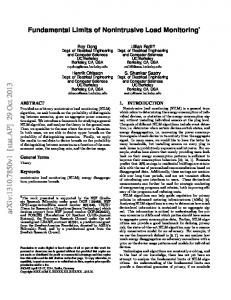
Figure 3: Washing machine footprint and HMM in the dataset AMPds.
in the training phase, which is performed by collecting a large number of footprints, i.e., the active power 150
signal comprised between the power on (transition from the OFF state to an ON state) and the power off (transition from an ON state to the OFF state). The estimation of the power levels associated to each HMM state is obtained by clustering the extracted footprints with the k -means algorithm [51]. Figure 3 shows an example of the inference procedure conducted on the active power signal. The signal is related to the washing machine in the AMPds dataset. In particular, Figure 3a shows the active power
155
signal and the cluster membership of each sample. In the figure, each cluster is depicted as an interval whose size is twice the standard deviation of the cluster centred at its centroid. The related HMM is represented in Figure 3b. 4.2. The AFAMAP algorithm AFAMAP has been proposed in [17] as an efficient disaggregation algorithm based on FHMMs. In this
160
algorithm, an additional model which relies on the same HMMs composing the Additive FHMM (AFHMM) is introduced. It is based on a differential version of the aggregated signal, resulting in a Differential FHMM (DFHMM). The inference on the set of states of multiple HMMs can be computed through the Maximum A Posteriori (MAP) algorithm and a relaxation towards real values is taken into account, leading to a convex Quadratic Programming (QP) optimisation problem. The disaggregation process is performed by analysing
165
the aggregated power divided in non-overlapping frames. The details of the AFAMAP algorithm are not reported here for the sake of conciseness. The interested reader can refer to [17] for the original formulation and to [39] for the original algorithm which not includes the robust mixture component and that is assessed in this paper.
8
4.3. Rest of the World (RoW) modelling 170
In [17], the noised scenario is addressed by defining a robust mixture component both in the AFHMM and in the DFHMM. As in [39], in this work the robust mixture component is not used, and all the contributions are modelled as an additional appliance represented by the RoW model. This model is essential in order to be able to compare AFAMAP and the dAE approach in the noised scenario. This approach provides further advantages, since appliances with lower power consumption values risk to be modelled with working
175
states associated to similar consumption values. This can lead the algorithm to an erroneous assignment of the disaggregation output between similar models. Furthermore, the authors in [17] demonstrated that the disaggregation performance degrades as the number of appliances increases. Thus, representing several appliances with a single model eases the disaggregation task. The RoW model represents all the appliances but the ones of interest (typically, the ones with higher
180
consumption), and it is composed of a higher number of states with respect to the other appliances, since it has to represent a more complex operating mode. The number of states has to be evaluated in the experimental phase, since the greater values allow to better describe the behaviour of the ensemble appliances, but they can degrade the disaggregation performance, as demonstrated by the authors in [17]. Referring to equation (1), the training signal used to create the RoW model is the residual power consumption from the aggregated data, excluded the appliances power consumption: e(t) = y(t) −
N X
yi (t).
(4)
i=1
In the case where the dataset comprises always-on appliances, the RoW model does not include the OFF 185
working state, as showed in the Figure 4. The consumption values in the working states of the RoW model are extracted algorithmically using the k-means, even if there are no evident consumption values clusters, determined by any working state. 5. Experiments This section describes the experiments conducted to evaluate the performance of the dAE approach and
190
of the AFAMAP algorithm. Firstly, the performance metrics, the datasets, and the experimental procedure are described. Then, the obtained results are presented and discussed. 5.1. Performance metrics Depending on the application scenario, NILM algorithms can be evaluated by using different metrics each capturing particular aspects of the algorithm performance. NILM performance metrics can be divided
195
between those specific to energy disaggregation and the ones that focus on appliance state detection [41]. In order to evaluate both aspects of the NILM problem, algorithms have been evaluated by using the following metrics: 9
8,000
Noised aggregate Denoised aggregate
W
6,000 4,000 2,000 0 200
400
600
800
1,000
1,200
1,400
1,600
Minutes
(a) Noised aggregated power vs denoised aggregated power. 8,000
Noised aggregate RoW signal
W
6,000 4,000 2,000 0 200
400
600
800
1,000
1,200
1,400
1,600
Minutes
(b) Noised aggregated power vs RoW signal. Figure 4: The denoised aggregated power and the RoW signal, compared to the main aggregated power, in the AMPds.
(E)
• Energy-based Precision (P (E) ), Recall (R(E) ), and F1 -Measure (F1
) [17];
• Normalised Error in Assigned Power (NEP) [41]; (S)
200
• State-based Precision (P (S) ), Recall (R(S) ), F1 -Measure (F1 ), and Matthews Correlation Coefficient (MCC) [41, 52]. Energy-based Recall measures the part of the power consumption that has been correctly classified, whereas the Precision measures the amount of power assigned to an appliance that actually belongs to it. Considering (E)
the i-th appliance, Pi
(E)
Pi
(E)
and Ri are calculated as follows: PT PT min (ˆ yi (t), yi (t)) min (ˆ yi (t), yi (t)) (E) = t=1 PT , Ri = t=1 PT , y ˆ (t) t=1 i t=1 yi (t)
(5)
where yˆi (t) is the disaggregated power consumption signal, yi (t) is the ground truth appliance power consumption signal, and T is the total number of samples. In order to evaluate the total performance of the disaggregation algorithm, the metric average across the appliances is computed as follows: P (E) =
N 1 X (E) P , N i=1 i
R(E) =
N 1 X (E) R . N i=1 i
(6)
The F1 -Measure is calculated as the geometric mean between Precision and Recall: (E)
F1
=2
P (E) R(E) . P (E) + R(E) 10
(7)
The Normalised Error in Assigned Power measures the deviation of the estimated power yˆi (t) from the true power yi (t) normalised by the total energy consumption of the appliance. Considering appliance i, NEP is calculated as follows:
PT
|yi (t) − yˆi (t)| . PT t=1 yi (t)
t=1
NEPi =
(8)
State-based metrics are defined based on the actual and predicted state of an appliance. More in details, considering appliance i, true positives (TP), false positives (FP), false negatives (FN), and true negatives (TN) are defined as follows: T Pi =
T X
AND(xi (t) = on, x ˆi (t) = on),
(9)
AND(xi (t) = off, x ˆi (t) = on),
(10)
AND(xi (t) = on, x ˆi (t) = off),
(11)
AND(xi (t) = off, x ˆi (t) = off),
(12)
t=1
F Pi =
T X t=1
F Ni =
T X t=1
T Ni =
T X t=1
where xi (t) and x ˆi (t) are respectively the actual and the predicted state of appliance i at the time index t. Appliance i is considered in the “on” state if yi (t) exceeds a predefined threshold. Generally, the threshold varies with the appliance and it assumes the same value used for extracting the activations [27] (see also Section 5.3). State-based Precision and Recall are defined as: (S)
Pi
=
T Pi , T Pi + F Pi
(S)
Ri
=
T Pi , T Pi + F Ni
(13)
while state-based F1 -Measure is given by: (S)
F1
=
2P (S) R(S) , P (S) + R(S)
with
P (S) =
N N 1 X (S) 1 X (S) Pi , R(S) = R . N i=1 N i=1 i
(14)
Finally, the Matthews Correlation Coefficient is defined as: MCCi = p
T Pi T Ni − F Pi F Ni (T Pi + F Pi )(T Pi + F Ni )(T Ni + F Pi )(T Ni + F Ni )
and MCC = 205
N 1 X MCCi . N i=1
,
(15)
(16)
MCC assumes values in the range [−1, 1], with +1 representing perfect prediction, 0 random prediction, and −1 total disagreement between the ground truth and the prediction.
11
Table 1: Energy ratio (ER) for each house in the considered datasets.
UK-DALE Dataset ER
REDD
AMPds House 1
House 2
House 4
House 5
House 1
House 2
House 3
0.680
0.564
0.867
0.833
0.634
0.463
0.613
0.731
5.2. Datasets In order to conduct an exhaustive evaluation on different scenarios, three public datasets have been chosen. The Almanac of Minutely Power dataset (AMPds) [42] contains recordings of consumption profiles 210
belonging to a single home in Canada for a period of two years, at 1 minute sampling period. The experiments are conducted by using six appliances: dryer, washing machine, dishwasher, fridge, electric oven, and heat pump. The second dataset, UK-DALE [36], is composed of consumption profiles recorded in five houses in UK over two years, at 6 seconds sampling period. The houses consumptions are not equally distributed over this time period, e.g., house 3 contains only the kettle consumptions and some minor appliances recordings,
215
thus it is not considered in the experiments. The five target appliances considered in all the experiments are: fridge, washing machine, dish washer, kettle and microwave. The third dataset, REDD [25], contains aggregate and circuit-level power profiles of several US households. The sampling period of the aggregate data is 1 s, while the one of the target profiles is 3 s, thus aggregate data was downsampled in order to match the sample period of the target profiles. The experiments are conducted by using four appliances: dryer,
220
dishwasher, fridge, and microwave. In the seen scenario, the data from two houses is used both for training and testing. In the unseen scenario, the same data is used for training, while testing is performed on the data of a third house. The chosen appliances represent the principal contributions to the peak of power consumption in the aggregated signal, which allows us to consider the denoised scenario as an approximation of the noised scenario in the traits of higher power consumption. On the other hand, the noise contribution, assigned to the RoW model, depends on the number of remaining appliances not modelled and on the total energy of the main aggregated signal, and this affects the disaggregation performance in the noised scenario. The energy ratio (ER), defined as: PT e(t) ERoW ER = = PTt=1 , Emain t=1 y(t)
(17)
expresses the energy proportion between the RoW model and the total aggregated data, and the values for each house in the considered datasets is showed in Table 1. 225
The datasets are split in different portions for training and testing, and their dimensions depend on the availability of appliances activations within the dataset. Regarding the training procedure, within the period specified in Table 2, the first 20 % of activations are used to compose the validation set, while the remaining 80 % are used for the models training. 12
Table 2: Definition of the training, validation and test sets for the considered datasets.
Dataset
Train+Validation
Test
AMPds
1 year, 6 months
6 months
House 1
1 year, 8 months, 3 days
7 days
House 2
4 months, 3 days
7 days
House 4
6 months, 25 days
7 days
House 5
2 months, 3 days
6 days
House 1
33 days
3 days
House 2
12 days
2 days
House 3
12 days
6 days
UK-DALE
REDD
Regarding the ground truth consumption availability, two different scenarios can be defined. In the seen 230
scenario, the disaggregation is computed on the same houses used to train the models, but in different period from the training data. In this scenario, both models, HMM and neural network, are created exploiting the same portion of training, in order to conduct a fair comparison between the methods. On the other hand, in the unseen scenario, the disaggregation is computed on the data related to a house not considered in the training phase. In this scenario, the ground truth consumptions related to each appliance are not available
235
in the house where the disaggregation in performed, therefore no training data can be considered to create the models. The generalisation property of the neural network allows to avoid a training procedure and to use the model trained on a set of data different from the test, whereas the footprints needs to be suitably extracted in order to train the HMM. One possible approach, in this sense, is represented by the user-aided footprint extraction algorithm [53], that describes a procedure for the extraction of an approximated version
240
of the appliance activations within the aggregated data when all the appliances are turned off, except the always-on in the house, i.e., the fridge and the freezer. The experiments on the UK-DALE dataset have been performed as in [27], both for the seen and the unseen scenario. 5.3. Experimental setup
245
The parameters related to the AFAMAP algorithm are defined as follows: the frame size is set to 60 minutes, which is an interval sufficiently large to include the whole activation for most of the appliances under study. For the ones with a longer activation, this frame size allows to include a complete operating sub cycle, for which the HMM is still representative. The variance parameters are set to σ12 = σ22 = 0.01 according to the variance of the experimental data, and the regularisation parameter is set to λ = 1. Table 3 presents
250
the number of states, defined a-priori for each class of appliance. In the denoised scenario no parameters
13
Table 3: Number of states m related to each class of appliance.
Nr. of
Washing Dryer
states m
Dishwasher machine
3
4
3
Electric
Heat
oven
pump
3
3
Fridge 2
Kettle
Microwave
2
2
Table 4: Window width (in samples) for the dAE architecture. The number of samples depends on the dataset sampling rate.
Washing Dataset
Dryer
Dishwasher
Electric
Heat
oven
pump
Fridge
machine
Kettle
Microwave
UK-DALE
-
1024
1536
512
-
-
128
288
AMPds
75
120
210
45
120
90
-
-
REDD
1536
-
2304
496
-
-
-
96
optimisation has been conducted, whereas in the noised scenario, the number of the RoW states has been varied between the values {6, 8, 10} for both datasets. The algorithm has been implemented in Matlab, and the CPLEX1 solver has been adopted to solve the QP problem. The experiments have been conducted on a working station equipped with an Intel i7 CPU at 3.3 GHz, and 32 GB RAM. The time required for an 255
experiments depends on the number of samples and the number of states of the HMM models: because of the different sampling rate between the datasets, the experiments last from 1 hour for AMPds to 3 hours for UK-DALE, while the introduction of the RoW model increases the simulation time up to 2 hours for AMPds and 5 hours for UK-DALE. The parameters related to the dAE approach are defined as follows: each network receives data in a mini-
260
batch of 64 sequences, and a mean and variance normalization is computed on the input data. In order to guarantee the same normalization over the whole dataset, the mean and variance values are computed from a random sample of the training set. Whereas, on the target data a min-max normalization is performed using the maximum power consumption value of the related appliance. The training data is composed of 50 % of actual appliance related data, and 50 % of synthetic data obtained by randomly combining real
265
appliance activations. The training sequences have been extracted by using NILMTK [41]: this toolkit provides the method for the power activation extraction from the ground truth power consumption related to each appliance from both datasets. The data analysing window of the dAE needs to be enough large to comprise an entire activation of the appliance, but not too much to include other contributions, especially for appliances with short-duration activation. The window width depends on the appliance type, as described
270
in the Table 4: As aforementioned, training has been performed by using the SGD algorithm with Nesterov 1 https://www-01.ibm.com/software/commerce/optimization/cplex-optimizer/
14
momentum set 0.9. The maximum number of epochs has been set to 200 000, and the number of epochs for the variable step size technique has been set to 20 000. The initial value of the learning rate has been set to 0.1, with a decreasing factor equal to 10. The variable step size criterion has been applied on the F1 -Measure calculated on the validation set, and the relative tolerance for early stopping criterion has been 275
set equal to 0.01. The neural network has been implemented by means of the Lasagne library2 , built on top of Theano [54]. All the network weights have been initialised randomly using Lasagne default initialisation, without any layerwise pre-training. In [27], the network topology is composed of an input and an output convolutional layer with 8 kernels of size 4. The middle layers consists of 3 fully connected layers with ReLU activation functions, where the
280
number of neurons in the central layer is equal to 128, whereas for the other layers the number depends on the length of the input sequence. In the disaggregation phase, a hop size of 16 samples has been considered. The performance of this work represents the baseline for this approach. An intensive parameters optimisation has been conducted regarding to the number of kernels (N), size of each kernel (S), and number of neurons in the central layer (H). The experiments have been conducted using each combination of parameters within
285
the ranges: N={2, 4, 8, 16, 32, 64}, S={2, 4, 8, 16, 32, 64}, H={8, 16, 32, 64, 128, 256, 512, 1024, 2048}. Kernels larger than the input size have not been considered. The architecture that achieves the highest performance has been used as starting point of an additional campaign of experiment, for which the first convolutional layer has been preserved, and a second stage, including pooling and up-sampling layers, has been introduced. The parameters have been varied within the same ranges defined above.
290
Max pooling is calculated on a segment with sizes equal to 2 or 4 samples, and the overlapped portion is either equal to half of the window or not present. For this new architecture the experiments have been conducted with a full search of the optimal parameters. The disaggregation phase has been carried out with a sliding window technique over the aggregated signal, using overlapped window with hop size in the range {1, 2, 4, 8, 14 window, 12 window}, where window represents to the window width defined in Table 4.
295
The number of networks tested for each appliance in three datasets has been varied from 150 to 200, and this experimental campaign has been conducted on both denoised and noised scenario, in the seen and unseen conditions. The experiments have been conducted on nVIDIA K80 GPUs. The training time varies depending on the network dimension and appliance type: because of the different sampling rates of the datasets, the
300
experiments require from 2 to 10 hours depending on the size of the training set. 2 https://lasagne.readthedocs.io/en/latest/
15
5.4. Results on the seen scenario Regarding the AFAMAP algorithm, in the noised scenario, preliminary experiments have demonstrated that the highest performance is obtained when the number of states of the RoW model is 6. For the sake of conciseness, here we report only the results for that number of states. 305
For the same reason, the results of the entire experimental campaign of the dAE algorithm will not be reported. For each scenario, the introduction of the second stage of CNN improves the performance with respect to the single CNN stage for the majority of appliances, as well as the effectiveness of the pooling layer. The experiments demonstrated that a hop size with 1 and 2 samples results in the best performance. For the AMPds and UK-DALE datasets, the dAE algorithm outperforms AFAMAP both in the noised
310
and the denoised scenarios, as shown in Table 5, Table 6, Figure 5a, and Figure 5b. More in details, Figure 5 (E)
shows the radar charts related to the F1
metric for each appliance, and the area inside a line gives an
overall performance indicator of the related approach. On the AMPds dataset, in the denoised case study, (E)
the absolute improvement in terms of F1
amounts to + 17.3 %, while in the noised scenario the absolute
improvements amounts to + 13.3 %. The same trend can be observed by considering the other metrics. 315
Compared to AFAMAP, NEP reduces by 2.012 in the denoised scenario, whereas it reduces by 3.819 in the (S)
noised scenario. State-based metrics show a similar trend, since, in the denoised case study, F1
improves
by + 24.7 %, while and in the noised case study the absolute improvement is + 29.8 %. Similar remarks apply to MCC. Analysing the performance of the individual appliances, the dAE algorithm outperforms AFAMAP (E)
for all the appliances in both the denoised and the noised scenario. In terms of F1 320
, the highest absolute
improvement can be observed for the dishwasher (+ 45.9 %) in the denoised scenario, and for the oven in the noised scenario (+ 48.4 %). Considering the other metrics, the dAE algorithm outperforms AFAMAP for all the appliances in both scenarios, except for the fridge in the noised scenario, where AFAMAP achieves (S)
lower NEP and higher F1 . Indeed, for this appliance in the noised scenario, the performance improvement (E)
in terms of F1
is modest compared to the other appliances. (E)
325
Compared to AFAMAP, in the UK-DALE dataset the absolute improvement in terms of F1
is + 4.4 %
in the denoised case study, and to + 48.7 % in the noised scenario. The same trend can be observed by considering the other metrics: NEP reduces by 0.672 in the denoised scenario and by 11.564 in the noised (S)
scenario, while F1
improves by + 11.7 % in the denoised case study and by + 36.51 % in the noised case
study. MCC increases by 0.166 and by 0.466 respectively in the denoised and in the noised scenario. 330
Analysing the performance of the individual appliances, the dAE algorithm achieves superior performance for all the appliances in the denoised scenario, except for the washing machine and the microwave, for which (E)
the F1
is similar. In the noised scenario, the dAE algorithm outperforms AFAMAP for all the appliances,
with the highest improvement equal to + 69.6 % for the kettle. The same trend can be observed considering the other metrics. In the noised scenario, the optimisation of the network parameters allows to outperform
16
(E)
335
the dAE architecture presented in [27] for all the appliances, with the highest improvement of F1
equal
to + 26.1 % for the dishwasher. Considering the other metrics, the improvement follows the same trends, (S)
except for the washing machine evaluated in terms of NEP, and the dishwasher evaluated in terms of F1 and MCC.
Regarding the REDD dataset (Table 7), in the denoised scenario the performance difference of the dAE (E)
340
algorithm with respect to AFAMAP varies with the evaluation metric. In particular, in terms of F1
and MCC, AFAMAP outperforms the dAE algorithm respectively by 6.5 % and 0.007. In terms of MCC, (S)
however, the relative improvement is limited, since it is equal to 0.95 %. In terms of NEP and F1 , the dAE approach outperforms AFAMAP as shown in the experiments with the UK-DALE and AMPds datasets. This behaviour can be explained by considering that in the denoised seen scenario the HMM models in AFAMAP 345
are trained by using data of the same building used in the disaggregation phase, while the network in the dAE approach is trained by using multiple buildings, and testing is performing on one of those. This aspect is less relevant in the noised scenario, because in AFAMAP the RoW model introduces a high variability in the disaggregation solution. Indeed, in this scenario the dAE approach outperforms AFAMAP regardless the evaluation metric.
350
Generally, the dAE approach reaches higher disaggregation performance since it allows to reproduce complex activation profiles, which are learned during the training procedure and are associated to the aggregated profiles, even in the presence of the noise contribution. As shown in Table 5, Table 6 and Table 7, the highest performance is reached in the disaggregation of the appliances with higher peak power consumption, since it allows a better association between the target and the aggregated input sequence during
355
the training phase. In the HMM based approach, each state of an appliance model represents one value of power consumption, which does not allow to represent highly variable or transient phenomena between the working states of the appliance. Additionally, in the AFAMAP algorithm the disaggregation solution is obtained by considering all the appliance models at the same time, while in the dAE approach each network operates independently from the others. This may cause a false energy assignment to an appliance, due to
360
the need to satisfy the constraint that the sum of the reconstructed profiles corresponds to the aggregated power. In presence of noise, the performance degrades significantly, since the presence of the RoW, composed of a higher number of states compared to appliance models, increases the number of admissible solutions and, as a consequence, the chance of errors in the disaggregated profiles reconstruction. Moreover, in the AFAMAP algorithm there is no information on the total duration of the complete activation, since appliance
365
models incorporate only the information on the working state transition and on the consumption values. Further evaluations can be carried out by analysing the disaggregated profiles in denoised and noised scenario. Considering the UK-DALE experiments in seen scenario, the profiles related to the dishwasher in the house 1 are shown in Figure 6. The appliance activation is correctly detected by the dAE in both scenar-
17
AFAMAP denoised
dAE denoised
AFAMAP noised
dAE noised
Washing
Washing
machine
machine
Washing Dishwasher machine
Fridge
Dishwasher
100% 80% 60% 40% Dryer 20%
100% 80% 60% 40% 20%
Dishwasher
100% 80% 60% 40% 20%
Kettle
Fridge
Fridge Microwave
Electric oven
Kettle
Microwave
Heat pump
(b) Disaggregation performance on
(c) Disaggregation performance on
(a) Disaggregation performance on
the UK-DALE dataset, seen sce-
the UK-DALE dataset, unseen sce-
the AMPds dataset, seen scenario.
nario.
nario.
Fridge
Dryer
Fridge
100% 80% 60% 40% 20%
Microwave
Dryer 100% 80% 60% 40% 20%
Microwave
Dishwasher
Dishwasher
(d) Disaggregation performance on
(e) Disaggregation performance on
the REDD dataset, seen scenario.
the REDD dataset, unseen scenario.
Figure 5: Performance for the different appliances for the all the addressed algorithms. The energy-based F1 -Measure (%) is represented.
18
Table 5: Disaggregation performance in the seen scenario (AMPds dataset). Numbers in bold indicate the best performing approach.
Washing Scenario
Algorithm
Metric
Dryer
Dishwasher machine
(E)
F1
(%)
NEP AFAMAP [17]
(S)
F1
(%)
MCC Denoised
(E) F1
(%)
NEP dAE
(S)
F1
(%)
MCC (E) F1
(%)
NEP AFAMAP + RoW
(S) F1
(%)
MCC Noised
(E) F1
(%)
NEP dAE
(S)
F1
(%)
MCC
Electric
Heat
oven
pump
Fridge
Overall
87.3
14.5
44.4
35.5
38.1
76.9
60.4
0.281
7.761
2.093
0.837
2.909
0.352
2.372
60.7
7.4
11.9
36.0
5.0
86.2
50.3
0.631
0.092
0.161
0.335
0.121
0.855
0.366
96.1
50.5
90.3
63.7
84.1
77.4
77.7
0.068
0.919
0.182
0.558
0.289
0.142
0.360
76.0
54.8
76.8
75.6
53.4
93.4
75.0
0.780
0.567
0.773
0.690
0.584
0.932
0.721
65.3
6.2
27.8
38.3
8.9
54.6
40.8
0.999
18.100
2.812
0.938
6.305
0.873
5.004
16.0
7.6
10.7
43.3
2.0
55.5
30.8
0.239
0.096
0.141
0.198
0.041
0.543
0.210
91.2
11.9
49.8
39.1
57.3
65.4
54.1
0.131
4.416
0.640
0.940
0.568
0.419
1.185
76.8
10.8
58.2
33.1
45.9
79.8
60.6
0.784
0.165
0.593
0.217
0.489
0.789
0.506
ios, without producing false positives in the disaggregated trace. In the noised scenario, the reconstructed 370
profiles have a high uncertainty, caused by the presence of noise in the aggregated power, but the average energy in the activation has a good correspondence with the ground truth one, which demonstrates the low degradation of performance compared to the denoised scenario. The same experiment has been considered for the fridge, whose profiles are shown in Figure 7. The dAE algorithm recognises the appliance activation in the denoised scenario, with a less accurate profile reconstruction in the activation overlapped with other
375
appliances respect to the isolated ones. Differently, the performance degrades in the noised scenario, with an incorrect activation detection and the production of some false positives, caused by the presence of noise in the aggregated signal. 5.5. Results on unseen scenario As aforementioned, the unseen scenario is evaluated by using the UK-DALE and REDD datasets, due
380
to the availability of recordings from several houses in both. As in the noised seen scenario, preliminary experiments conducted by varying the number of states in the (E)
RoW model demonstrated that the highest F1
is obtained with 6 states. Similarly, for the dAE algorithm
the results of the entire experimental campaign will not be reported the sake of conciseness. For each scenario,
19
Table 6: Disaggregation performance in the seen scenario (UK-DALE dataset). Numbers in bold indicate the best performing approach.
Washing Scenario
Algorithm
Metric
Kettle
Dishwasher
Fridge
Microwave
Overall
machine (E)
F1
(%)
NEP AFAMAP [17]
(S) F1
(%)
MCC Denoised
(E) F1
(%)
NEP dAE
(S) F1
(%)
MCC (E) F1
(%)
NEP AFAMAP + RoW
(S) F1
(%)
MCC (E) F1
(%)
NEP Noised
Kelly [27]
(S) F1
(%)
MCC (E) F1
(%)
NEP dAE
(S) F1
(%)
MCC
93.4
64.3
48.1
79.1
84.1
77.4
0.435
14.090
1.322
0.358
1.038
3.449
81.9
41.2
22.5
84.6
78.1
70.4
0.797
0.451
0.287
0.781
0.788
0.621
94.1
59.6
86.2
85.8
82.9
81.8
0.087
13.087
0.220
0.207
0.287
2.777
95.7
56.2
57.4
93.2
90.4
82.1
0.957
0.559
0.620
0.896
0.903
0.787
12.8
20.4
18.5
49.4
11.5
24.9
1.754
53.063
1.752
0.865
4.193
12.325
7.79
15.80
16.95
51.91
18.24
35.49
0.150
0.145
0.179
0.324
0.177
0.195
80.1
35.1
58.2
64.1
59.5
60.4
0.522
1.384
0.707
0.609
0.923
0.829
82.12
35.32
69.53
65.68
62.58
69.18
0.821
0.372
0.706
0.575
0.626
0.620
82.4
54.8
84.3
73.6
72.4
73.6
0.393
2.135
0.278
0.472
0.524
0.760
86.6
40.8
55.6
78.2
75.5
72.0
0.866
0.425
0.583
0.683
0.751
0.661
the introduction of the second stage of CNN and of the pooling operation improves the performance with 385
respect to the single CNN stage for the majority of the appliances. Regarding the hop size in the sliding window disaggregation phase, as in the seen scenario the highest performance is reached by using 1 and 2 samples. Similarly to the seen scenario in the UK-DALE dataset, the baseline [27] performance for each appliance in the noised scenario is outperformed by means of the optimisation of the network parameters, with the (E)
390
highest absolute improvement of F1
equal to + 30.2 % for the washing machine. The same trend can be (S)
observed for the other metrics, excepting for the F1
and the MCC, where the dishwasher performance
degrades. For both datasets, the dAE algorithm outperforms AFAMAP in both scenarios, as shown and Table 8 (E)
and Table 9. In the UK-DALE dataset, the absolute improvement in terms of F1 395
amounts to + 8.6 % in the
denoised case study, whereas it increases to + 50.5 % in the noised scenario, demonstrating the superiority 20
Table 7: Disaggregation performance in the seen scenario (REDD dataset). Numbers in bold indicate the best performing approach.
Scenario
Algorithm
Metric (E)
F1
(%)
NEP AFAMAP [17]
(S) F1
(%)
MCC Denoised
(E) F1
(%)
NEP dAE
(S) F1
(%)
MCC (E)
F1
(%)
NEP AFAMAP + RoW
(S)
F1
(%)
MCC Noised
(E)
F1
(%)
NEP dAE
(S) F1
(%)
MCC
Dishwasher
Dryer
Fridge
Microwave
Overall
67.1
94.4
80.5
80.2
82.6
1.086
0.093
0.338
0.491
0.502
50.12
97.59
89.79
66.86
78.85
0.512
0.975
0.833
0.666
0.746
66.3
87.3
74.6
64.9
76.1
0.515
0.265
0.543
0.397
0.430
71.7
92.7
80.5
69.6
80.9
0.669
0.926
0.666
0.695
0.739
36.4
31.9
36.0
17.9
35.4
2.207
1.187
0.905
2.287
1.646
32.9
57.6
39.6
16.2
46.0
0.354
0.567
0.260
0.176
0.339
62.1
72.5
66.9
53.0
66.1
0.551
0.506
0.760
0.615
0.608
64.0
81.8
70.9
61.6
72.4
0.495
0.814
0.468
0.604
0.595
of the neural network based approach with respect to the HMM one, especially in presence of the noise contribution. The results evaluated with the other metrics confirm the same trend, with a reduction of NEP equal to 0.543 in the denoised case study and to 5.418 in the noised case study. Considering the state (S)
based metrics, the improvement evaluated with the F1 400
amounts to + 12.52 % in the denoised scenario
and + 53.10 % in the noised, as well as regarding the MCC with an absolute improvement of + 0.170 in the denoised scenario and + 0.594 in the noised scenario. As showed in Figure 5c, overall the dAE algorithm outperforms AFAMAP both in the denoised and in the noised scenarios. In particular, the dAE exhibits (E)
a noteworthy robustness against the presence of noise, while the F1
of AFAMAP reduces significantly.
Observing the results of each appliance, the highest absolute improvement is obtained for the kettle and it is 405
equal to + 80.4 %. In the denoised scenario, the dAE algorithm outperforms AFAMAP for all the appliances, (E)
with only exception of the dishwasher where the F1
is 1.6 % lower. Considering the other metrics, in the
noised scenario, the performance is improved for all the appliances, while in the denoised scenario the same trend can be observed, except for the washing machine, which degrades its performance in terms of NEP, (S)
F1
and MCC.
21
3,000 Noised aggregate Denoised aggregate
W
2,000 1,000 0
1.67
1.68
1.69
1.7
1.71
1.72
1.73
1.74
1.75 ·105
Seconds
Ground truth Denoised disaggregated
W
2,000 1,000 0
1.67
1.68
1.69
1.7
1.71
1.72
1.73
1.74
1.75 ·105
Seconds
Ground truth Noised disaggregated
W
2,000 1,000 0
1.67
1.68
1.69
1.7
1.71
1.72
1.73
1.74
1.75 ·105
Seconds
Figure 6: Disaggregated profiles in denoised and noised scenario in UK-DALE dataset, seen case study, related to the dishwasher in house 1.
(E)
410
On the REDD dataset, the absolute improvement in terms of F1
amounts to + 30.20 % in the denoised
scenario and + 21.18 % in the noised scenario. The other metrics follow the same trends, with a reduction of NEP equal to 1.964 in the denoised case study and to 1.371 in the noised case study. Considering the (S)
state based metrics, the improvement evaluated with the F1
amounts to + 28.3 % in the denoised scenario
and + 19.60 % in the noised, as well as regarding the MCC with an absolute improvement of + 0.341 in 415
the denoised scenario and + 0.234 in the noised scenario. In the REDD dataset, differently from the seen scenario described above, the dAE algorithm outperforms on each appliance in both scenario, with the (E)
highest improvements in terms of F1
of + 53.51 % for the microwave, except for the dryer in the denoised
scenario with the state based metrics. The radar chart represented in Figure 5e shows this improvement, and it represent the performance loss of both algorithm in the noised scenario with respect to the denoised 420
scenario. In the unseen scenario the generalisation property of the dAE approach allows to apply the model without the need of training, with a reasonable degradation of performance. Regarding the AFAMAP algorithm, the approximation introduced by the footprint extraction procedure causes a lack of correspondence between the HMM and the appliance working states consumptions, and this results in a higher performance degradation,
425
particularly in presence of noise where RoW model is present. This demonstrates the effectiveness of the neural networks approaches in an unseen scenario, which is the most interesting condition, because it
22
3,000 Noised aggregate Denoised aggregate
W
2,000 1,000 0 1.62
1.63
1.64
1.65
1.66
1.67
1.68
1.69
1.7
1.71 ·105
Seconds 200
Ground truth Denoised disaggregated
W
150 100 50 0 1.62
1.63
1.64
1.65
1.66
1.67
1.68
1.69
1.7
1.71 ·105
Seconds 200
Ground truth Noised disaggregated
W
150 100 50 0 1.62
1.63
1.64
1.65
1.66
1.67
Seconds
1.68
1.69
1.7
1.71 ·105
Figure 7: Disaggregated profiles in denoised and noised scenario in UK-DALE dataset, seen case study, related to the fridge in house 1.
represents a real world application of the NILM service. As described in the previous section, the state based metrics confirm that the dAE produces a more reliable activation detection, with respect to the HMM based approach, even in an unseen scenario.
430
6. Conclusion In this paper, a DNN architecture based on the denoising autoencoder topology has been proposed. Compared to the work by Kelly and Knottenbelt [27] several improvements have been introduced. In the training phase, the variable step size has been adopted, with an early stopping criterion based on the performance metric calculated on the validation set. In the disaggregation phase, the median filter has
435
been applied to combine the overlapped portion of signal in the sliding window analysis of the aggregated power data. In order to achieve the best performance, for each network an optimisation of the network parameters has been conducted, starting from the reference architecture and introducing a second layer of CNN and a pooling stage to compress the size of the output. The proposed approach has been compared to the AFAMAP [17] algorithm, which is one of the most representative methods for NILM using the HMM
440
paradigms. This algorithm has been adopted for the noised scenario with the introduction of RoW model. The experiments have been conducted on the AMPds [42], on the UK-DALE [36] and on the REDD [25] datasets, evaluating both the denoised and noised scenario. Furthermore, the availability of recordings from 23
Table 8: Disaggregation performance in the unseen scenario (UK-DALE dataset). Numbers in bold indicate the best performing approach.
Washing Scenario
Algorithm
Metric
Kettle
Dishwasher
Fridge
Microwave
Overall
machine (E)
F1
(%)
95.1
32.3
80.9
73.6
29.9
66.1
0.114
2.089
0.457
0.449
3.311
1.284
97.11
25.59
12.84
74.68
38.33
61.68
0.971
0.353
0.177
0.690
0.440
0.526
95.7
39.5
79.3
91.1
67.1
74.7
0.056
2.406
0.371
0.195
0.675
0.741
99.7
23.4
54.5
95.5
65.1
74.2
0.997
0.286
0.604
0.931
0.664
0.696
3.2
4.7
20.2
32.2
4.2
17.3
3.087
6.559
2.078
1.021
18.413
6.231
0
5.1
11.8
33.6
3.3
18.7
MCC
-0.001
0.085
0.151
0.120
0.090
0.089
(E) (%) F1
79.1
23.3
39.2
65.1
20.6
50.8
NEP
0.448
1.607
0.892
0.562
2.875
1.277
93.9
26.5
55.9
77.8
30.9
66.8
0.940
0.373
0.597
0.712
0.416
0.608
83.6
53.5
69.2
78.7
45.8
67.8
0.177
1.439
0.648
0.419
1.383
0.813
95.6
67.5
50.9
82.8
45.4
71.8
0.957
0.687
0.502
0.757
0.510
0.683
NEP AFAMAP [17]
(S) F1
(%)
MCC Denoised
(E) F1
(%)
NEP dAE
(S) F1
(%)
MCC (E) F1
(%)
NEP AFAMAP + RoW
Noised
Kelly [27]
(S) F1
(S) F1
(%)
(%)
MCC (E) F1
(%)
NEP dAE
(S) F1
(%)
MCC
more than one building in the UK-DALE and in the REDD datasets allowed to evaluate the algorithms on an unseen scenario. The results showed that the proposed approach outperforms the comparative methods 445
in the overall average between the appliance, both in denoised and noised scenario. Regarding the unseen scenario, the performance demonstrated that the generalisation property of the dAE allowed acceptable degradation of performance, respect to the AFAMAP algorithm, in which the footprint extraction stage introduced errors in the HMM modelling phase. As future works, a more reliable appliance model will be considered in order to improve the represen-
450
tation of additional working states, e.g., the usage of Gaussian Mixture Model (GMM) within the HMM. Furthermore, additional information about the working states duration will be introduced, to fully exploit the differential model. For the dAE approach, the introduction of a constraint between the neural model output will be considered, in order to assume the equality between the aggregated data and the sum of the profiles reconstructed, in the denoised scenario. In order to apply this constraint in the noised scenario, the 24
Table 9: Disaggregation performance in the unseen scenario (REDD dataset). Numbers in bold indicate the best performing approach.
Scenario
Algorithm
Metric (E)
F1
(%)
NEP AFAMAP [17]
(S) F1
(%)
MCC Denoised
(E) F1
(%)
NEP dAE
(S) F1
(%)
MCC (E)
F1
(%)
NEP AFAMAP + RoW
(S)
F1
(%)
MCC Noised
(E)
F1
(%)
NEP dAE
(S) F1
(%)
MCC
455
Dishwasher
Dryer
Fridge
Microwave
Overall
32.2
49.5
69.3
7.0
46.4
3.336
0.811
0.491
4.754
2.348
18.6
89.8
73.6
4.3
55.9
0.282
0.901
0.650
0.056
0.472
76.1
83.7
78.5
60.5
76.6
0.348
0.292
0.426
0.470
0.384
87.5
85.8
88.1
67.4
84.2
0.877
0.860
0.805
0.711
0.813
22.5
18.8
40.0
8.4
26.4
3.803
1.521
0.946
3.728
2.500
14.2
41.3
37.3
5.1
35.0
0.228
0.399
0.180
0.083
0.222
41.8
57.2
60.4
13.6
47.6
0.756
0.955
1.053
1.752
1.129
49.2
59.3
71.7
16.8
54.6
0.543
0.617
0.497
0.166
0.456
introduction of the neural based RoW model will be required.
Acknowledgements We acknowledge the CINECA award under the ISCRA initiative, for the availability of high performance computing resources and support, and Netribe Business Solution srl for supporting this research. [1] K. C. Armel, A. Gupta, G. Shrimali, A. Albert, Is disaggregation the holy grail of energy efficiency? 460
The case of electricity, Energy Policy 52 (2013) 213–234. [2] A. Zoha, A. Gluhak, M. A. Imran, S. Rajasegarar, Non-intrusive load monitoring approaches for disaggregated energy sensing: A survey, Sensors 12 (12) (2012) 16838–16866. [3] Z. Wang, G. Zheng, Residential appliances identification and monitoring by a nonintrusive method, IEEE Transactions on Smart Grid 3 (1) (2012) 80–92.
25
465
[4] K. Ehrhardt-Martinez, K. A. Donnelly, J. A. Laitner, Advanced metering initiatives and residential feedback programs: a meta-review for household electricity-saving opportunities, Tech. Rep. E105, American Council for an Energy-Efficient Economy Washington, DC (2010). [5] J. Laitner, K. Ehrhardt-Martinez, V. McKinney, Examining the scale of the behaviour energy efficiency continuum, in: American Council for an Energy Efficient Economy, European Council for an Energy
470
Efficient Economy Conference, Cote d’Azur, France, 2009, paper ID 1367. [6] G. Gardner, P. Stern, The short-list: the most effective actions us households can take to curb climate change, Environment: Science and Policy for a Sustainable Environment 50 (5) (2008) 12–24. [7] S. Ahmadi-Karvigh, B. Becerik-Gerber, L. Soibelman, A framework for allocating personalized appliance-level disaggregated electricity consumption to daily activities, Energy and Buildings 111
475
(2016) 337–350. [8] I. Abubakar, S. Khalid, M. Mustafa, H. Shareef, M. Mustapha, Application of load monitoring in appliances energy management a review, Renewable and Sustainable Energy Reviews 67 (2017) 235– 245. [9] L. D. Baets, J. Ruyssinck, C. Develder, T. Dhaene, D. Deschrijver, On the Bayesian optimization and
480
robustness of event detection methods in NILM, Energy and Buildings 145 (2017) 57–66. [10] M. Zeifman, K. Roth, Nonintrusive appliance load monitoring: Review and outlook, IEEE Trans. Consum. Electron. 57 (1) (2011) 76–84. [11] L. K. Norford, S. B. Leeb, Non-intrusive electrical load monitoring in commercial buildings based on steady-state and transient load-detection algorithms, Energy and Buildings 24 (1) (1996) 51 – 64.
485
[12] R. Bonfigli, S. Squartini, M. Fagiani, F. Piazza, Unsupervised algorithms for non-intrusive load monitoring: An up-to-date overview, in: Environment and Electrical Engineering (EEEIC), 2015 IEEE 15th International Conference on, 2015, pp. 1175–1180. [13] M. Aiad, P. H. Lee, Unsupervised approach for load disaggregation with devices interactions, Energy and Buildings 116 (2016) 96 – 103.
490
[14] H. Kim, M. Marwah, M. F. Arlitt, G. Lyon, J. Han, Unsupervised disaggregation of low frequency power measurements, in: Proc. 11th SIAM Int. Conf. Data Mining, Mesa, AZ, USA, 2011, pp. 747–758. [15] O. Parson, S. Ghosh, M. Weal, A. Rogers, An unsupervised training method for non-intrusive appliance load monitoring, Artificial Intelligence 217 (2014) 1–19.
26
[16] O. Parson, M. Weal, A. Rogers, A scalable non-intrusive load monitoring system for fridge-freezer energy 495
efficiency estimation, in: Proc. of the 2nd Int. Workshop on Non-Intrusive Load Monitoring, 2014. [17] J. Kolter, T. Jaakkola, Approximate inference in additive factorial HMMs with application to energy disaggregation, Journal of Machine Learning Research 22 (2012) 1472–1482. [18] I. Valera, F. Ruiz, F. Perez-Cruz, Infinite factorial unbounded-state hidden markov model, Pattern Analysis and Machine Intelligence, IEEE Transactions on 38 (9) (2016) 1816–1828.
500
[19] Y. Li, Z. Peng, J. Huang, Z. Zhang, J. H. Son, Energy disaggregation via hierarchical factorial hmm, in: Proc. of the 2nd Int. Workshop on Non-Intrusive Load Monitoring, 2014. [20] M. Zhong, N. Goddard, C. Sutton, Signal aggregate constraints in additive factorial HMMs with application to energy disaggregation, in: Advances in Neural Information Processing Systems, 2014, pp. 3590–3598.
505
[21] M. Zhong, N. Goddard, C. Sutton, Interleaved factorial non-homogeneous hidden markov models for energy disaggregation, in: Advances in Neural Information Processing System, Workshop on Machine Learning for Sustainability, Lake Tahoe, Nevada, USA, 2014. [22] A. Cominola, M. Giuliani, D. Piga, A. Castelletti, A. Rizzoli, A hybrid signature-based iterative disaggregation algorithm for non-intrusive load monitoring, Applied Energy 185, Part 1 (2017) 331–344.
510
[23] S. Makonin, F. Popowich, I. V. Baji´c, B. Gill, L. Bartram, Exploiting HMM Sparsity to Perform Online Real-Time Nonintrusive Load Monitoring, IEEE Transactions on Smart Grid 7 (6) (2016) 2575–2584. [24] M. Johnson, A. Willsky, Bayesian nonparametric hidden semi-Markov models, Journal of Machine Learning Research 14 (1) (2013) 673–701. [25] J. Z. Kolter, M. J. Johnson, REDD: A public data set for energy disaggregation research, in: Workshop
515
on Data Mining Applications in Sustainability (SIGKDD), San Diego, CA, 2011. [26] F. C. C. Garcia, C. M. C. Creayla, E. Q. B. Macabebe, Development of an intelligent system for smart home energy disaggregation using stacked denoising autoencoders, in: Proc. of the Int. Symp. on Robotics and Intelligent Sensors (IRIS), Tokyo, Japan, 2016, pp. 248–255. [27] J. Kelly, W. Knottenbelt, Neural NILM: Deep neural networks applied to energy disaggregation, in:
520
Proceedings of the 2nd ACM International Conference on Embedded Systems for Energy-Efficient Built Environments, BuildSys ’15, ACM, New York, NY, USA, 2015, pp. 55–64. [28] L. Mauch, B. Yang, A new approach for supervised power disaggregation by using a deep recurrent LSTM network, in: Proc. of GlobalSIP, Orlando, FL, USA, 2015, pp. 63–67. 27
[29] L. Mauch, B. Yang, A novel DNN-HMM-based approach for extracting single loads from aggregate 525
power signals, in: Proc. of ICASSP, Shanghai, China, 2016, pp. 2384–2388. [30] M.-S. Tsai, Y.-H. Lin, Modern development of an adaptive non-intrusive appliance load monitoring system in electricity energy conservation, Applied Energy 96 (2012) 55–73. [31] B. Zhao, L. Stankovic, V. Stankovic, On a Training-Less Solution for Non-Intrusive Appliance Load Monitoring Using Graph Signal Processing, IEEE Access 4 (2016) 1784–1799.
530
[32] M. Figueiredo, A. De Almeida, B. Ribeiro, Home electrical signal disaggregation for non-intrusive load monitoring (NILM) systems, Neurocomputing 96 (2012) 66–73. [33] J. M. Gillis, S. M. Alshareef, W. G. Morsi, Nonintrusive Load Monitoring Using Wavelet Design and Machine Learning, IEEE Trans. Smart Grid 7 (1) (2016) 320–328. [34] S. M. Tabatabaei, S. Dick, W. Xu, Toward non-intrusive load monitoring via multi-label classification,
535
IEEE Transactions on Smart Grid 8 (1) (2017) 26–40. [35] S. Hochreiter, J. Schmidhuber, Long short-term memory, Neural Computation 9 (1997) 1735–1780. [36] J. Kelly, W. Knottenbelt, The UK-DALE dataset, domestic appliance-level electricity demand and whole-house demand from five UK homes, Scientific data 2. [37] V. Nair, G. Hinton, Rectified linear units improve restricted boltzmann machines, in: Proc. of the 27th
540
Int. Conf. on Machine Learning (ICML), Haifa, Israel, 2010, pp. 807–814. [38] A. Gabaldon, R. Molina, A. Marn-Parra, S. Valero-Verdu, C. Alvarez, Residential end-uses disaggregation and demand response evaluation using integral transforms, Journal of Modern Power Systems and Clean Energy 5 (1) (2017) 91–104. [39] R. Bonfigli, M. Severini, S. Squartini, M. Fagiani, F. Piazza, Improving the performance of the AFAMAP
545
algorithm for non-intrusive load monitoring, in: Proc. of IEEE Congress on Evolutionary Computation (CEC), 2016, pp. 303–310. [40] M. Zhong, N. Goddard, C. Sutton, Latent bayesian melding for integrating individual and population models, in: Proc. of Advances in Neural Information Processing Systems, Montr´eal, Canada, 2015, pp. 3618–3626.
550
[41] J. Kelly, N. Batra, O. Parson, H. Dutta, W. Knottenbelt, A. Rogers, A. Singh, M. Srivastava, NILMTK v0.2: A non-intrusive load monitoring toolkit for large scale data sets: Demo abstract, in: Proceedings of the 1st ACM Conference on Embedded Systems for Energy-Efficient Buildings, BuildSys ’14, ACM, New York, NY, USA, 2014, pp. 182–183. 28
[42] S. Makonin, F. Popowich, L. Bartram, B. Gill, I. V. Bajic, AMPds: A public dataset for load disag555
gregation and eco-feedback research, in: Proceedings of the 2013 IEEE Electrical Power and Energy Conference (EPEC), 2013. [43] P. Vincent, H. Larochelle, I. Lajoie, Y. Bengio, P.-A. Manzagol, Stacked Denoising Autoencoders: Learning Useful Representations in a Deep Network with a Local Denoising Criterion, J. Mach. Learn. Res. 11 (3) (2010) 3371–3408.
560
[44] S. Araki, T. Hayashi, M. Delcroix, M. Fujimoto, K. Takeda, T. Nakatani, Exploring multi-channel features for denoising-autoencoder-based speech enhancement, in: Proc. of the IEEE Int. Conf. on Acoustics, Speech and Signal Processing, Brisbane, Australia, 2015, pp. 116–120. [45] X. Lu, Y. Tsao, S. Matsuda, C. Hori, Speech Enhancement Based on Deep Denoising Autoencoder, in: Proc. of Interspeech, Lyon, France, 2013, pp. 436–440.
565
[46] I. Sutskever, J. Martens, G. Dahl, G. Hinton, On the importance of initialization and momentum in deep learning, in: Proc. of the 30th Int. Conf. on Machine Learning (ICML), Atlanta, USA, 2013, pp. 2176–2184. [47] Z. Ghahramani, M. Jordan, Factorial Hidden Markov Models, Machine Learning 29 (2-3) (1997) 245– 273.
570
[48] S. Pattem, Unsupervised disaggregation for non-intrusive load monitoring, in: Machine Learning and Applications (ICMLA), 2012 11th International Conference on, Vol. 2, IEEE, 2012, pp. 515–520. [49] O. Parson, S. Ghosh, M. Weal, A. Rogers, Non-intrusive load monitoring using prior models of general appliance types, in: Twenty-Sixth Conference on Artificial Intelligence (AAAI-12), 2012. [50] L. Rabiner, A tutorial on hidden markov models and selected applications in speech recognition, Pro-
575
ceedings of the IEEE 77 (2) (1989) 257–286. [51] J. A. Hartigan, M. A. Wong, Algorithm as 136: A k-means clustering algorithm, Journal of the Royal Statistical Society. Series C (Applied Statistics) 28 (1) (1979) 100–108. [52] B. W. Matthews, Comparison of the predicted and observed secondary structure of T4 phage lysozyme, Biochimica et Biophysica Acta (BBA)-Protein Structure 405 (2) (1975) 442–451.
580
[53] R. Bonfigli, E. Principi, S. Squartini, M. Fagiani, M. Severini, F. Piazza, User-aided Footprint Extraction for Appliance Modelling in Non-Intrusive Load Monitoring, in: Proc. of the IEEE Symposium Series on Computational Intelligence, Athens, Greece, 2016, pp. 1–8.
29
[54] Theano Development Team, Theano: A Python framework for fast computation of mathematical expressions, arXiv e-prints abs/1605.02688.
30