North American Journal of Fisheries Management 22:351–364, 2002 q Copyright by the American Fisheries Society 2002
Inferring Bayesian Priors with Limited Direct Data: Applications to Risk Analysis RANSOM A. MYERS* Department of Biology, Dalhousie University, Halifax, Nova Scotia B3H 4J1, Canada
N. J. BARROWMAN Department of Mathematics and Statistics, Dalhousie University, Halifax, Nova Scotia B3H 3J5, Canada
RAY HILBORN School of Aquatic and Fishery Sciences, University of Washington, Post Office Box 357980, Seattle, Washington 98195, USA
DANIEL G. KEHLER Department of Mathematics and Statistics, Dalhousie University, Halifax, Nova Scotia B3H 4J1, Canada Abstract.—The usefulness of Bayesian analysis depends in great part on specifying appropriate prior distributions. In this article, we investigate three quantitative techniques for obtaining a prior distribution for steepness, a critical parameter in fisheries management. These techniques were developed in the context of a risk assessment of a power plant’s impact on nine species of fish. All three techniques use mixed-effects models to estimate the parameters of the prior distributions, but they differ in the choice of the fish populations to include in the analysis. The first two methods use information from taxonomically similar and ecologically similar populations, respectively, to generate a prior distribution. The third method combines a mixed-effects model and a quantitative analysis of life history and environmental data to generate a prior distribution, using data from all available fish populations. These techniques represent an empirical Bayesian approach, which we preferred to a hierarchical Bayesian approach because it allowed us to rapidly explore numerous alternative model formulations.
Bayesian approaches to the analysis of population dynamics (and in particular, those for fisheries) are becoming a standard, if not the standard, in some areas (Liermann and Hilborn 1997; Punt and Hilborn 1997; Hilborn and Liermann 1998; Meyer and Millar 1999). However, the provenance of the prior distributions, that is, the distributions of parameters from a probability model, remains the most difficult problem in Bayesian analyses. A variety of approaches exist for parameterizing prior distributions. The simplest procedure is to use subjective information (reflecting personal opinion) to parameterize priors, but this is usually not rigorous enough to be of practical use for risk assessment. There are formal methods for selecting priors that reflect ignorance (i.e., ‘‘uninformative’’ priors; Kass and Wasserman 1996), but such priors provide little information for the de-
cision maker in a risk assessment. The purpose of this paper is to demonstrate how informative prior distributions can be obtained empirically with little direct data. We will use, as an example, a prior for ‘‘steepness,’’ a critical management parameter used in risk analysis. Steepness (h) is related to the maximum reproductive rate of a stock and is thus a measure of how productive a stock is at low population size. Productivity at low population size is important in assessing potential risks since it defines the level of additional mortality, such as that caused by fishing or a power plant, a population can sustain over the long term. Unfortunately, there are many populations for which such data are simply not available directly, yet decisions have to be made and risk assessments carried out. Here we introduce several methods for approaching this problem.
* Corresponding author:
[email protected]
The Problem in Context: Priors for Steepness for Nine Fish Species The techniques presented in this paper were developed in the context of a risk assessment of the
Received August 18, 2000; accepted July 18, 2001
351
352
MYERS ET AL.
impact of a power plant intake (the Salem Nuclear Power Plant on the Delaware estuary, which uses once-through cooling for two of its reactors; Anonymous 1999) on nine species of fish: alewife Alosa pseudoharengus, American shad Alosa sapidissima, blueback herring Alosa aestivalis, striped bass Morone saxatilis, white perch M. americana, bay anchovy Anchoa mitchilli, spot Leiostomus xanthurus, weakfish Cynoscion regalis, and Atlantic croaker Micropogonias undulatus. The risk assessment evaluated the mortality caused by entrainment through the power plant’s cooling structure or impingement on the cooling structure’s intake screen. Most of this mortality occurred during the larval or juvenile stage. For this assessment, we needed to obtain objective priors of steepness that would be rigorous enough for a court of law. We developed three alternative quantitative approaches for obtaining estimates of the prior distributions: (1) priors were based on information from taxonomically similar populations; (2) priors were based on information from ecologically similar populations; and (3) priors were inferred from a quantitative analysis of life history and environmental data. For the purposes of the risk analysis, we preferred the method (if valid) that yielded the most conservative estimates of the maximum reproductive rate (and hence steepness). The three approaches can be used in either a fully Bayesian or an empirical Bayesian context (Carlin and Louis 1996). A fully Bayesian approach would require the specification of distributions for the parameters of the priors (i.e., hyperpriors), which would typically be uninformative. Here we use an empirical Bayesian approach because of its relative simplicity for this risk assessment. In the empirical Bayesian context, we obtain maximum likelihood (ML) estimates of the ‘‘priors,’’ that is, the distribution of parameter values from mixed-effects models. Following Efron (1996), we refer to these as MLE priors. The fully Bayesian approach has the disadvantage that it is often difficult to determine whether a Markov chain Monte Carlo (MCMC) algorithm has converged. Moreover, it may be difficult to choose truly uninformative hyperpriors, and if improper priors (or hyperpriors) are used, the posterior distribution may not be proper and thus may not be used for inference (Hobert and Casella 1996). In addition, using the MCMC algorithm to obtain parameter estimates is time consuming, making it difficult to explore alternative models or to carry out sensitivity analyses. This problem is
particularly important here because many models had to be investigated. The principle disadvantage of the empirical Bayesian approach is that the variances will be underestimated (Efron 1996), producing narrower prior distributions than a fully Bayesian approach. Empirical Bayesian Estimates of Maximum Reproductive Rate and Steepness Although we used the Beverton–Holt model for our population dynamics, we employed the Ricker model to estimate the maximum reproductive rate because it gives more conservative (i.e., lower) estimates than most other models (Myers et al. 1999). The Ricker model has the form Rt9 5 a9St e2bSt,
(1)
where Rt9 and St are the abundance or biomass of recruits and spawners, respectively, in year t, and a9 is the slope at the origin (measured, perhaps, in numbers of recruits per kilogram of spawners) and measures the maximum reproductive rate. Density-dependent mortality is assumed to be the product of b and the spawner biomass. Dividing by St and taking logarithms gives log e
R9t 5 log ea9 2bS t , St
(2)
which is a linear model for log-survival. For the forthcoming calculations, Rt9 must be standardized so that data from different species can be analyzed simultaneously. We did so by converting the numbers of recruits (Rt9 ) into the abundance of spawners that would be produced by S t spawners if there were no fishing. We call this quantity R t , even though it is in units of spawners. It is calculated by the following relation: Rt 5 Rt9 · SPRF50 ,
(3)
where SPRF50 is the spawning abundance resulting from each recruit (perhaps in kilograms per spawner per recruit) when there is no fishing mortality (F 5 0; see Appendix 1 for details on calculating SPRF50). Using the standardized recruits results in a different a9, denoted a, which represents the number of spawners produced by a single spawner over its lifetime at low spawner abundance (slope at the origin), assuming no density dependence or fishing mortality. We considered p populations, subscripted by i, for each of which we wanted to estimate the parameters of a Ricker model of the form
353
INFERRING BAYESIAN PRIORS WITH LIMITED DATA
log e
R i,t 5 log ea i 2 b i S i,t 1 e i,t , S i,t
(4)
where Ri,t is recruitment to year-class t in population i, Si,t is spawner abundance in year t in population i, ai and bi are the Ricker model parameters for population i, and ei,t is estimation error (assumed normal). We assumed that logeai was a normal random variable and defined m 1 ai [ logeai, where m was the mean of the log-transformed maximum annual reproductive rates and ai was the random effect for population i. In the empirical Bayesian approach used here, we obtained maximum likelihood estimates of the parameters of the distribution of ai, that is, estimates of m and the variance of ai. These served to define the empirical prior for future analysis. We considered the log-survival, loge (R/S), of a year-class from a given population as an element of a vector y. If there were ni observations for population i, then the first n1 elements of the vector y would be the n1 log-survivals for the first population, followed by the n2 log-survivals for the second population, and so on. In a standard fixed-effects model, the parameters are the overall mean, m, and the p regression parameters, bi. The spawner abundances, Si,t, were assumed known, and we estimated the density-dependent regression parameter, bi, for each population. The standard mixed-effects model notation for the vector of fixed-effects parameters is b. The unknown vector b consists of the overall mean, m, and the p bis. The vector b is related to y by the known model matrix X, whose elements are 0, 1, and Si,t; the form of this matrix is given in Myers et al. (1999). In our mixed model, we assumed that the ais were random effects. For the vector of random effects composed of the ais we use the standard mixed-model notation u. The vector u is related to y by a known model matrix Z. In standard mixed-model notation, we have y 5 Xb 1 Zu 1 e.
(5)
Here, e is an unknown random error vector. The generalization provided by the mixed model enables one not only to model the mean of y (as in the standard linear model) but also to model the variance of y. We assumed that u and e were uncorrelated and that they had multivariate normal distributions with expectations 0 and variances D and R, respectively. The variance of y was thus V 5 ZDZ9 1 R.
(6)
One can model the variance of the data, y, by specifying the structure of D and R. We assumed that D 5 s2aI (where I is the identity matrix), that is, that the variability among populations of log eai was normally distributed with variance s2a. In the simplest case, one might assume that the error variance is the same for all populations, that is, that R 5 s2I. However, we can also estimate a separate estimation error variance, s2i , for each population. It is also a simple matter to include autocorrelation in the residuals (Myers et al. 1999). If such autocorrelation is included, it increases the estimation error variance and causes the empirical Bayesian estimates of the random effects to be pulled more toward the mean for the species (i.e., there is a smaller estimated random-effects variance). This will have no effect on the mean of the prior distribution, and since our analysis did not explicitly consider all sources of variation (e.g., errors in estimating spawner abundance) we preferred to keep the random-effects variances as large as possible to reflect this uncertainty. Having transformed the problem into this form, estimation was trivial because high-quality software exists for this problem (Myers et al. 1999). The likelihood function for the data vector y ; NN (Xb, V) is 21
L 5 L(b, V z y) 5
e21/ 2(y2X b)9V (y2X b) , (2p) N/ 2 zVz1/ 2
(7)
where N is the number of fixed effects estimated, that is, N 5 1 1 p. In this form, we can obtain estimates of the desired parameters to estimate the empirical prior, that is, the parameters m and sa. Simulation experiments of the above problem have shown that the mixed model produces nearly unbiased estimates of model parameters if the assumptions of the model are met, namely, if the Ricker model is correct and the errors are independently and normally distributed (Myers et al. 1999). However, if the true model is actually Beverton–Holt, then the mean of a (the slope at the origin of the spawner recruitment function) is underestimated by about 40%, but the variance remains unbiased (Myers et al. 1999). The Ricker model will not give conservative estimates for all possible models; for example, it will sometimes overestimate the maximum reproductive rate compared with the hockey stick model (Barrowman and Myers 2000). The use of the MLE prior in the assessments should thus provide reliable results if the assumptions are met but will provide conservative estimates if the data actually follow a Beverton–Holt model.
354
MYERS ET AL.
The risk analysis models we used are parameterized in terms of steepness, denoted by h (first defined by Mace and Doonan [1988]), because this is the parameter used in many assessments (Hilborn and Walters 1992). The steepness parameter for the Beverton–Holt model is defined as the ratio of recruitment when spawner abundance or biomass is reduced to 20% of the equilibrium (no fishing) level to recruitment when there is no fishing. Steepness is related to the maximum lifetime reproductive rate a by the equation h5
a , 41a
where 0.2 , h , 1. Note that at the limit of small population size the Ricker and Beverton–Holt models coincide, that is, the slope at the origin, a, is the same. In this context, h can be estimated from either model; however, it can only be applied directly to the dynamics of the Beverton–Holt model. Our estimate of steepness should be viewed as conservative unless there is depensation (reduced survival at low spawner abundance). However, these priors are designed to be used when the spawner abundance is not very low, so that depensation is unlikely to occur. Three Approaches to Inferring Priors Our goal is to infer an appropriate prior distribution, sometimes known as a predictive distribution (Carlin and Louis 1996), of h for use in a risk assessment model. Here, we describe three approaches to this problem. For the first two approaches, we use two different criteria, taxonomic and ecological similarity, to select populations to include in the mixed-effects model analysis that generates the distribution for a and hence h. In the third approach, which involves adding covariates to the mixed-effects model, the different populations included in the analysis are weighted depending upon their values of life history and environmental variables. We describe the three approaches in more detail below. Taxonomic criterion.—The prior distribution can be determined using a taxonomic criterion. That is, data from other populations of the same species or species that are closely related to the population of interest can be used to infer the prior. This is the most common method and the only fairly objective method we know of that has been used in fisheries (Punt and Hilborn 1997). This approach was possible only for species where good
data existed on other populations of the same species or populations of closely related species. In our example, this approach was possible only for the three Alosa species (alewife, American shad, and blueback herring). We also had data for one population of striped bass. Although no prior distribution can be constructed from a single dataset, we can compare a point estimate of the maximum reproductive rate with the means (or modes) of other prior distributions. Ecological criteria.—An alternative to using the taxonomic criterion is to have an independent expert select, on ecological grounds, populations that are ‘‘similar’’ to the population of interest. The expert should not have access to the results of the analysis, that is, knowledge of estimated maximum reproductive rates. In our example, James Cowan (University of South Alabama, Mobile) was chosen to independently specify the populations to be used in the analysis because he had conducted extensive research on all the species of interest (Cowan and Houde 1990; Cowan et al. 1996). Cowan was provided with information on the following traits: natural mortality, longevity, type of reproduction (i.e., oviparous versus ovoviviparous), habitat (i.e., anadromous, freshwater, or marine), fecundity, age at maturity, and environmental temperature. From this set of environmental and life history data, he selected the fish populations that he felt would best serve to calculate the variability in log e a for each of the nine new populations of interest. Again, data from these populations were used in the mixed-model analysis to calculate a prior distribution for loge a . Covariate analysis.—A third approach is to infer the priors from an analysis based on empirical regressions involving the same life history and environmental data used in the second method. In this approach, life history and taxonomic data were used to select a subset of characteristics that explained the variation in the maximum reproductive rate. We used a three-step strategy for model building that was suggested by Davidian and Giltinan (1995; see also Maitre et al. 1991). The first step is to fit a hierarchical model with no covariates. The second step is to plot the empirical Bayesian estimates against potential covariates and to use this graphical evidence to guide model formulation. The last step is to create a functional model incorporating important covariates. In doing so, we followed the strategy of Davidian and Giltinan (1995). Let Ci be the value of a particular covariate
INFERRING BAYESIAN PRIORS WITH LIMITED DATA
for population i. The form of the model is a modification of equation (3): log e
R i,t 5 log ea i 2 b i S i,t 1 dC i 1 e i,t , S i,t
(8)
where the term dCi has been added. The parameter d represents the relationship (assumed linear) between the deviation of log-survival and the covariate under investigation. We used the above formulation because it appeared to give a reasonable fit to the data and it was easily incorporated into well-studied models. In the covariate analysis, we obtained maximum likelihood estimates for the priors for the pattern of covariates for the population of interest. That is, we estimated the mean and variance of logea as before but added the effect of the estimate of the covariate, dˆ Ci, where dˆ is the maximum likelihood estimate of d and Ci is the value of the covariate for the population of interest. Populations and Data Used in the Analyses We began our analyses with data for which quantitative estimates, in the form of the maximum reproductive rate, could be obtained from the extensive database used in Myers et al. (1999). The following life history information was used in the analyses: (1) Natural mortality or reproductive longevity. We used the same natural mortality estimates that were used in the assessments (typically the natural mortality that occurs after reproduction begins) to estimate the spawner2recruitment data. This parameter provides information on the mean number of spawning (reproductive) bouts for an adult that has reached maturity. For Pacific salmon Oncorhynchus spp., the reproductive longevity is one because the fish die after spawning. If the probability of survival each year after reproduction begins is P, then the mean number of spawnings will be 1 1 P 1 P2 1 · · · Pn 5 1/(1 2 P) (this result is the infinite sum of a geometric series and ignores the small effect of senescence). We will call this quantity reproductive longevity. (2) Oviparous versus ovoviviparous reproduction. (3) Habitat (a categorical variable—anadromous, freshwater, or marine). (4) Fecundity. Fecundity estimates were obtained from literature reviews such as Scott and Scott (1988) and those compiled in Mertz and Myers (1996). We estimated the mean fecundity per year for reproductive individuals. If several batch-
355
es of eggs mature throughout the year, we attempted to estimate the sum over the year. (5) Age at maturity. We used the estimated age at which 75% of females reach maturity. (6) Latitude and environmental temperature. We estimated the mean temperature of the geographic center of spawning for each population in the analysis. These variables were used to obtain maximum likelihood estimates of the prior for each of the nine species in the study. We attempted to compile all of the spawner2recruitment data in the world for the analysis (see Myers et al. 1995 and the updates available on the web site http://fish.dal.ca./welcome.html), which resulted in data for over 700 fish populations. However, only 246 of these populations had sufficiently detailed data to enable us to obtain reliable estimates of the maximum reproductive rate. The dataset included 57 species from 21 families and 8 orders. Of the 246 populations, 109 were anadromous, 11 were freshwater, and 126 were marine or estuarine. Results Taxonomic Criterion We estimated empirical priors for the three of our species in the genus Alosa. As this taxonomic group corresponded exactly to the ‘‘domain 2 anadromous’’ group discussed in the next section, we will not discuss it in detail here. It was not possible to construct a prior from the single stock assessment for striped bass, as no information exists about the random-effect variance. However, we can compare the point estimate to the mean of the empirical priors generated using the other two approaches. The estimated mean of h was 0.82, with the 20th and 80th percentiles estimated to be 0.8 and 0.84, respectively. Ecological Criteria Our independent expert, James Cowan, initially selected only those populations that spawn where winter temperatures are between 58C and 228C, as these temperatures correspond to those within the range of the nine species of interest. Temperatures were measured at a depth of 50 m for marine species, except for those in shallow seas, for which a depth of 20 m was used. In some cases, direct temperature data were not available but we could infer them from the data from surrounding regions. Cowan’s rationale for this criterion is that the temperatures at which these stocks operate is important to some life history characteristics. He also
356
MYERS ET AL.
FIGURE 1.—Maximum likelihood priors (truncated to have support on [0.2, 1] and then rescaled) for steepness for the life history domains described by James Cowan of the University of South Alabama, Mobile. The fish in domain 2 were separated into anadromous and nonanadromous populations. One population in domain 1 (the ayu from Lake Biwa, Japan) was considered an outlier and removed from the analysis; the estimate of steepness for this population is indicated.
eliminated species whose life histories were radically different from the species of interest (e.g., Salmonidae). Cowan decided on three ‘‘domains’’ by which to categorize the nine species of interest. A prior distribution for logea was calculated for each domain using data from the populations (but not the population of interest) that fit the criteria for each domain. Domain 1.—This category includes fish with an early age at maturity (,2 years), high natural mortality ($0.3 on a yearly basis), and relatively low fecundity (,100,000 eggs/year). The bay anchovy was the only species of interest to fall within the domain. However, nine other populations from the database also fell within it. The individual esti-
mates of the maximum reproductive rate for these populations fell into two clear clusters, namely, those with an a of around 4 and the population of ayu Plecoglossus altivelis from Lake Biwa, Japan, which had an a of 123.5 (SE 5 2.3). The analysis for the ayu appears to be very reliable and is supported by fishery-independent survey data (Suzuki and Kitahara 1996). Even so, in estimating the MLE prior we have treated this species as an outlier. Although this may significantly lower our estimation of the steepness, it is consistent with the precautionary principle. The estimate based on the remaining eight populations produced a relatively narrow prior for steepness (Figure 1). Domain 2.—This life history domain has an old-
INFERRING BAYESIAN PRIORS WITH LIMITED DATA
er age at maturity (2–5 years), lower natural mortality rates (0.2–0.5/year), moderate fecundity (generally between 100,000 and 750,000 eggs/ year), and moderate longevity (5–15 years). Most of the species of interest fell within this domain (weakfish, Atlantic croaker, spot, Atlantic shad, alewife, blueback herring, and white perch). This domain corresponds to the periodic life history of Winemiller and Rose (1992). Cowan further subdivided domain 2 into anadromous and marine populations. Seventy-two populations from the database fell within this domain, of which eight were anadromous. The anadromous category consists entirely of Alosa species. The remaining 64 populations were used to construct the priors for the domain 2 nonanadromous priors. The priors estimated for the anadromous and nonanadromous populations were similar, except that the latter was slightly wider. In particular, the nonanadromous prior has some probability mass lying below 0.2 (a steepness of 0.2 is the minimum needed for a population to survive; however, it is possible for the model to make estimates below 0.2 unless it is constrained). This small probability mass was eliminated from the estimates (and the prior density rescaled) because it represents a population that is not at equilibrium. Furthermore, none of the individual estimates were this low. Domain 3.—This life history domain is characterized by an older age at maturity (.4 years), low natural mortality rate (#0.2), and high fecundity (.500,000 eggs/year). Striped bass was the only species of interest in domain 3. Nine populations from the database fell into this domain. The maximum likelihood estimates for domain 3 produced a very reasonable prior with the high maximum reproductive rate typical of long-lived species such as striped bass. Covariate Analysis Two approaches can be used to determine which covariates are of interest, namely, comparing the deviance of models with and without the covariate and employing graphical techniques. Although fully exploring the various model configurations is beyond the scope of this paper, our preliminary analyses suggest that both fecundity (on a logarithmic scale) and reproductive longevity are important covariates. Previous studies suggest that reproductive longevity is strongly related to the maximum reproductive rate (Myers et al. 1999). For the graphical analysis, we made use of the ‘‘lowess’’ smooth for scatterplot data (Cleveland 1979) to detect trends in the data. This is a robust,
357
local smoothing technique using locally linear fits. A window that is dependent on the fraction of the data selected to be analyzed is placed about each x value; the points that are inside the window are weighted so those that are close on the x-axis get the most weight. We used a fraction equal to 2/3, which produces very smooth plots. Natural mortality and reproductive longevity.— As in previous studies (Myers et al. 1999), there was a positive relationship between reproductive longevity and the maximum reproductive rate as measured by steepness (Figure 2). We thus used this relationship as a base from which to examine other factors that may affect the maximum reproductive rate and hence steepness. Egg or larval production.—We next considered oviparous versus ovoviviparous reproduction. The only species in the dataset with ovoviviparous reproduction were in the genus Sebastes. These populations were clearly very different from the others and were eliminated from further analysis because comparisons of fecundity between egg-bearing and live-bearing species are inappropriate (Figure 2). Habitat.—We next investigated habitat, that is, the anadromous, freshwater, or marine life history of fish (Figure 3). Here we saw that one possible cause of the positive relationship between reproductive longevity and the maximum reproductive rate is the short reproductive lifetime of the anadromous Pacific salmon species, which die after reproduction. As the marine species did not deviate very much from the trend (the dashed, robust lowess smooth for these species is very close to the overall trend), the relationship was probably not an artifact. Indeed, an analysis of deviance after removing all Pacific salmon populations still showed a significant positive effect of reproductive longevity (x21 5 10.3, P 5 0.0013). Note that most of the freshwater populations lie above the overall smooth, indicating that these populations have greater maximum reproductive rates than marine species of the same longevity. However, given the relatively few freshwater datasets, it is difficult to come to a reliable conclusion (Figure 3). Fecundity.—We divided fecundity into the three categories described by Cowan in his analysis. There did not appear to be any systematic difference in steepness across fecundity categories, although the low-fecundity species tend to have a lower reproductive longevity (Figure 4). Age at maturity.—We divided age at maturity into categories similar to those described by Cowan (#2 years, 2–5 years, and .5 years; Figure 5).
358
MYERS ET AL.
FIGURE 2.—Best linear unbiased estimates of steepness versus reproductive longevity for fish species by reproductive strategy (oviparous or ovoviviparous). The standard errors are approximate and were calculated using the delta method. Plotted points have been slightly staggered horizontally to improve visibility.
FIGURE 3.—Best linear unbiased estimates of steepness versus reproductive longevity for species with oviparous reproduction by habitat type (anadromous, freshwater, or marine). Lines are lowess fits (see text); see the caption to Figure 2 for additional details.
INFERRING BAYESIAN PRIORS WITH LIMITED DATA
359
FIGURE 4.—Best linear unbiased estimates of steepness versus reproductive longevity for species with oviparous reproduction by fecundity category (low [,100,000 eggs/year], medium [100,000–750,000 eggs/year], and high [.750,000 eggs/year]). There are blanks where fecundity estimates were not available.
FIGURE 5.—Best linear unbiased estimates of steepness versus reproductive longevity for species with oviparous reproduction by age at maturity (low [,2 years], medium [2–5 years], and high [.5 years]).
360
MYERS ET AL.
FIGURE 6.—Best linear unbiased estimates of steepness versus reproductive longevity for species with oviparous reproduction by age at maturity with Pacific salmon species excluded.
At low reproductive longevity (,5 years), there appeared to be a relationship between steepness and age at maturity (Figure 5). However, for populations with greater reproductive longevity, there was no relationship. The populations in this group are well represented by Atlantic cod Gadus morhua, for which weight at maturity varies much less among populations than age at maturity (Myers et al. 1997c). To investigate this question in more detail, we eliminated the Pacific salmon species (as they have very different life histories) and reexamined the data (Figure 6). The plot without the Pacific salmon species indicates that the relationship with age at maturity is not linear, nor is it strong. The species with one of the highest steepness values, the ayu from Lake Biwa in Japan, also has one of the lowest ages at maturity of any population. We thus did not include age at maturity as a factor in our covariate analysis. Latitude and temperature.—We examined the effects of latitude and/or environmental temperature by plotting the steepness for each population versus latitude. This analysis was carried out separately for each species. A strong negative relationship was found between the maximum reproductive rate and latitude for sockeye salmon Oncorhynchus nerka, a pattern that has been previously observed (Myers et al. 1997a). A sim-
ilar pattern occurred with Atlantic herring Clupea harengus, but this may be due to a decreased maximum reproductive rate at the edge of the species’ range, a pattern that would be consistent with the observed greater importance of environmental effects on recruitment at such locations (Myers 1998). For Atlantic cod the pattern appeared to be in the opposite direction, with greater a in the north. This pattern is probably an artifact of the differences in the temperature2latitude relationships on the eastern and western sides of the Atlantic. If anything, there was a weak positive relationship between a and temperature for the among-population comparisons of Atlantic cod (Myers et al. 1997c). We concluded that among the populations of a given species, neither latitude nor temperature had a consistently strong effect; however, there may have been a small increase in a with temperature and it may have reached a maximum at the center of a species’ range. We thus did not include latitude or temperature in our covariate analysis. Summary of the empirical analysis of environmental and life history data.—There was a strong positive relationship between reproductive longevity and the maximum reproductive rate. The other factor that appeared to influence the maximum reproductive rate was the type of reproduction (oviparous versus ovoviviparous). The only
INFERRING BAYESIAN PRIORS WITH LIMITED DATA
361
FIGURE 7.—Comparison of maximum likelihood priors for steepness derived from the covariate analysis (solid lines) with those derived from the ecological criteria (dotted lines). Although the prior distributions have been truncated to have support on [0.2, 1] and then rescaled, this has little effect on their shapes because the mass less than 0.2 is very small. For striped bass, the point estimate of the mean from the taxonomic analysis is also presented (dashed line). The modes for the various domains are as follows: 0.483 (domain 1), 0.74 (domain 2, anadromous), 0.747 (domain 2, nonanadromous), and 0.836 (domain 3).
species in the data set with ovoviviparous reproduction are in the genus Sebastes. These are clearly very different from the oviparous species, so much so that the assessments for them might require a close examination to determine whether the data
were collected during atypical years or there was some unusual factor at work. None of the other factors that we examined appeared to have a strong and consistent relationship with the maximum reproductive rate, so we did
362
MYERS ET AL.
not include them in the final covariate estimation of the priors. As there was some evidence that the Pacific salmon species were different from other comparable species, we considered the effect of eliminating this group in our robustness tests. Estimation of priors based on covariate analysis.—Following the strategy of Davidian and Giltinan (1995), we built a functional model incorporating reproductive longevity as a covariate. Our analysis used a mixed model of the form of equation (8), where Ci is the reproductive longevity of population i and d is the effect of this covariate. In this model we had to decide on the data to be used for the regression analysis. We considered three possibilities: (1) all oviparous species, (2) all oviparous species except the Pacific salmon species, and (3) all oviparous species except the Pacific salmon species and the most influential datasets. The robustness tests were carried out by eliminating from 1 to 4 populations that had the greatest effect on the estimation of d. The results from all three analyses were similar; however, the width of the priors were greater when we used the second option. We thus concluded that the most conservative strategy would be to use the second analysis in our model for estimating the covariate priors. The estimate of d that we used was 0.076 (SE 5 0.028). Comparison and Choice among the Alternative Methods of Selecting Priors The three approaches to obtaining MLE priors yielded similar results in most cases (Figure 7). For the Alosa species, the populations used to derive the prior using the taxonomic and ecological criteria happened to be identical. The results for the covariate analysis were relatively similar as well, though there was a tendency for the covariate prior to yield more conservative estimates of steepness. There were two cases in which the differences were relatively large. First, the mode of the MLE prior using the ecological criteria (with the outlier eliminated) was considerably less than that from the covariate analysis for the bay anchovy; the variance of the covariate prior was also larger. Second, although the modes of both striped bass MLE priors were very similar, the variance for the covariate prior was larger. To be consistent with the precautionary principle, in the risk analysis we used the priors that resulted in more conservative estimates of steepness, as there was no objective reason to choose one prior over another. That is, we used the prior
for domain 1 for bay anchovy and that from the covariate analysis for alewife, American shad, blueback herring, weakfish, spot, Atlantic croaker, and white perch. Conclusion Given recent advances in data compilation and statistical methods, it is possible to obtain reasonable estimates and infer reasonable priors for the maximum reproductive rate (and hence steepness, a critical parameter for the management of fish populations), even if very few data are available for a particular species. In this analysis, we demonstrated the use of three different ways to do this. The three approaches (using a taxonomic criterion, ecological criteria, and covariate analysis) yielded fairly similar priors, and adopting a conservative approach, we selected the one that gave the most conservative prior for each of the nine species of fish investigated. Thus, our results should underestimate the average steepness. The same analysis could also have been carried out using fully Bayesian methods or those that standardize the carrying capacity as well as the maximum reproductive rate (Myers et al. 2001). References Anonymous. 1999. Permit renewal application: NJPDES permit NJ0005622. Public Service Electric and Gas Company, Trenton, New Jersey. Barrowman, N. J., and R. A. Myers. 2000. Still more spawner2recruitment curves: the hockey stick and its generalizations. Canadian Journal of Fisheries and Aquatic Sciences 57:665–676. Carlin, B. P., and T. A. Louis. 1996. Bayes and empirical Bayes methods for data analysis. Chapman and Hall, London. Cleveland, W. S. 1979. Robust locally weighed regression and smoothing scatterplots. Journal of the American Statistical Association 74:829–836. Cowan, J. R., and E. D. Houde. 1990. Growth and survival of bay anchovy, Anchoa mitchilli, larvae in mesocosm enclosure. Marine Ecology Progress Series 68:47–57. Cowan, J. R., E. D. Houde, and K. A. Rose. 1996. Sizedependent vulnerability of marine fish larvae to predation: an individual-based numerical experiment. ICES Journal of Marine Science 53:23–38. Davidian, M., and D. M. Giltinan. 1995. Nonlinear models for repeated measurement data. Chapman and Hall, London. DeGisi, J. S. 1994. Year class strength and catchability of mountain lake brook trout. Master’s thesis. University of British Columbia, Vancouver. Efron, B. 1996. Empirical Bayes methods for combining likelihoods. Journal of the American Statistical Association 91:538–565. Hilborn, R., and M. Liermann. 1998. Standing on the
INFERRING BAYESIAN PRIORS WITH LIMITED DATA
shoulders of giants: learning from experience in fisheries. Reviews in Fish Biology and Fisheries 8: 1–11. Hilborn, R., and C. J. Walters. 1992. Quantitative fisheries stock assessment: choice, dynamics, and uncertainty. Chapman and Hall, New York. Hobert, J. P., and G. Casella. 1996. The effect of improper priors on Gibbs sampling in hierarchical linear mixed models. Journal of the American Statistical Association 91:1461–1473. Kass, R. E., and L. Wasserman. 1996. The selection of prior distributions by formal rules (with comments). Journal of the American Statistical Association 91: 1343–1370. Liermann, M., and R. Hilborn. 1997. Depensation in fish stocks: a hierarchic Bayesian meta-analysis. Canadian Journal of Fisheries and Aquatic Sciences 54:1976–1985. Mace, P. M., and I. J. Doonan. 1988. A generalized bioeconomic simulation model for fish population dynamics. New Zealand Ministry of Agriculture and Fisheries, Fish Assessment Research Document 88/ 4, Wellington, New Zealand. Maitre, P. O., M. Buhrer, D. Thomson, and D. R. Stanski. 1991. A three-step approach combining Bayesian regression and NONMEM population analysis: application to midazolam. Journal of Pharmacokinetics and Biopharmaceutics 19:377–384. Mertz, G., and R. A. Myers. 1996. Influence of fecundity on recruitment variability of marine fish. Canadian Journal of Fisheries and Aquatic Sciences 53:1618– 1625. Meyer, R., and R. B. Millar. 1999. Bayesian stock assessment using a state-space implementation of the delay difference model. Canadian Journal of Fisheries and Aquatic Sciences 56:37–52. Myers, R. A. 1998. When do environment2recruit relationships work? Reviews in Fish Biology and Fisheries 8:285–305. Myers, R. A., K. G. Bowen, and N. J. Barrowman. 1999.
363
The maximum reproductive rate of fish at low population sizes. Canadian Journal of Fisheries and Aquatic Sciences 56:2404–2419. Myers, R. A., M. J. Bradford, J. M. Bridson, and G. Mertz. 1997a. Estimating delayed density-dependent mortality in sockeye salmon (Onchorynchus nerka); a meta-analytic approach. Canadian Journal of Fisheries and Aquatic Sciences 54:2449–2463. Myers, R. A., J. Bridson, and N. J. Barrowman. 1995. Summary of worldwide stock and recruitment data. Canadian Technical Report of Fisheries and Aquatic Sciences 2024:327. Myers, R. A., J. A. Hutchings, and N. J. Barrowman. 1997b. Why do fish stocks collapse? The example of cod in Canada. Ecological Applications 7:91– 106. Myers, R. A., B. R. Mackenzie, K. G. Bowen, and N. J. Barrowman. 2001. What is the carrying capacity for fish in the ocean? A meta-analysis of population dynamics of north Atlantic cod. Canadian Journal of Fisheries and Aquatic Sciences 58:1464–1476. Myers, R. A., G. Mertz, and P. S. Fowlow. 1997c. Maximum population growth rates and recovery times for Atlantic cod, Gadus morhua. U.S. National Marine Fisheries Service Fishery Bulletin 95:762–772. Punt, A., and R Hilborn. 1997. Fisheries stock assessment and decision analysis: the Bayesian approach. Reviews in Fish Biology and Fisheries 7:35–65. Scott, W. B., and M. G. Scott. 1988. Atlantic fishes of Canada. Canadian Bulletin of Fisheries and Aquatic Sciences 219. Suzuki, N., and T. Kitahara. 1996. Relation of recruitment to the number of juveniles caught in the ayu population of Lake Biwa. Fisheries Science 62:15–20. Winemiller, K. O., and K. A. Rose. 1992. Patterns of life-history diversification in North American fishes: implications for population regulations. Canadian Journal of Fisheries and Aquatic Sciences 49: 2196–2218.
Appendix: Data Sources and Treatment The data that we used are estimates from assessments compiled by Myers et al. 1995. The full database is available from the first author, and a summary of the data by family, species, and population is available at http://fish.dal.ca./welcome. html. For marine populations, population numbers and fishing mortality were usually estimated using sequential population analysis (SPA) of commercial catch-at-age data. The SPA techniques include virtual population analysis (VPA), cohort analysis, and related methods that reconstruct population size from catch-at-age data (see Hilborn and Walters 1992, chapters 10211, for a description of the methods used to reconstruct the population his-
tory). Briefly, the commercial catch-at-age data are combined with estimates from research surveys and commercial catch rates to estimate the numbers at age in the final year and to reconstruct previous numbers at age under the assumption that commercial catch at age is known without error and that natural mortality at age is known and constant. For salmonid stocks, spawner abundance is the estimated number of upstream migrants discounted for mortality within the river; recruitment combines the catch and the number of upstream migrants. The SPA techniques were used for all freshwater species except brook trout Salvelinus fontinalis.
364
MYERS ET AL.
The brook trout were from introduced populations in California mountain lakes (DeGisi 1994); their numbers were estimated using research gill nets and maximum likelihood depletion estimation. The SPRF50 was calculated using estimates of natural mortality, weight at age, and maturity at age. Maturity and weight at age were usually estimated from research surveys carried out for each population. A major source of uncertainty in the SPA esti-
mates of recruitment and spawning stock biomass is that they usually assume that catches are known without error. This is particularly important when estimates of discarding and misreporting are not included in the catch-at-age data used in the SPA. These errors are clearly important for some of the Atlantic cod stocks during certain periods (Myers et al. 1997b) and will affect our estimates of the number of replacements each spawner can produce at low population densities (a).