Influence of Primary Network Structure and Dynamics on ... - IEEE Xplore

2011 IEEE International Symposium on Dynamic Spectrum Access Networks (DySPAN)

Influence of Primary Network Structure and Dynamics on Achievable Performance of Cognitive Wireless Networks Janne Riihij¨arvi, Jad Nasreddine and Petri M¨ah¨onen Institute for Networked Systems, RWTH Aachen University Kackertstrasse 9, D-52072 Aachen, Germany email: {jar, jad, pma}@inets.rwth-aachen.de

Abstract—We study the influence of the structure and dynamics of the primary network on occurrence and quality of transmit opportunities of the secondary network. In order to obtain accurate results, we develop a framework for performance evaluation that allows detailed modeling of the networks involved, while still enabling general conclusions to be drawn. The approach and results are applicable to diverse application scenarios, such as use of dynamic spectrum access techniques for femtocell deployments within operator networks. The techniques presented here can also be applied beyond dynamic spectrum access based networks for studying the performance of more general heterogeneous wireless systems as well. We use a combination of actual node location data sets and carefully selected node location models in order to obtain reliable results, while still allowing general conclusions to be made. The results show that even in dense primary networks significant opportunities for secondary use can arise. These originate either from the temporal dynamics of the primary, or in spatial domain from frequency reuse, provided that the primary network is active at most 30–50% of the time. For higher activity levels there are almost no useful spectrum opportunities even if the primary network is rather sparsely deployed. The results also show that the spatial structure of the deployment of the secondary network has significant influence on the capacity that can be achieved by using the arising spectrum opportunities.

I. I NTRODUCTION Cognitive wireless networks (CWNs) and techniques for dynamic spectrum access (DSA) have become over the last decade one of the most intensely studied topics in wireless communications [1]–[4]. There has been significant progress in understanding the performance properties of many of the involved technologies, especially those related to spectrum sensing and signal detection [5]–[8]. However, the achievable performance of CWNs and networks based on DSA is still relatively poorly understood on the system level. The main exception to this is the performance analysis of secondary networks operating in TV white spaces (such as those based on the IEEE 802.22 standard [9], [10]) which have been thoroughly studied during recent years especially by Sahai et al. [11], [12]. There has also been work towards more general capacity results for CWNs (see, for example, [13]–[17]), but these are often asymptotic in nature, or obtained using such a high abstraction level that it is difficult to make the connection with particular deployment scenario. Notable exceptions

978-1-4577-0178-8/11/$26.00 ©2011 IEEE

are [18] and [19] which consider explicitly secondary access in scenarios in which the primary network is a cellular system, albeit using somewhat simplified models for the structure of the primary and secondary networks. Nevertheless, as far as we are aware of, these references are only attempts in the literature to develop an accurate and realistic model for spectrum sharing in scenarios in which primary system is a cellular network. In this paper we carry out a systematic study on the influence of the primary network structure and dynamics on the expected performance of CWNs and more specifically on networks utilizing dynamic spectrum access. In particular, we both develop a novel analysis methodology and provide detailed results for a number of selected case studies. The developed approach allows to take into account the detailed topological and geometric structure of the involved networks, and it is not based on strong stochastic approximations as most of the earlier related work in the literature. In terms of structure, we consider both the deployment of the primary network, as well as network planning related properties such as the influence of frequency reuse factor on results. We also explore the influence of the activity patterns of primary network transmitters on the results. In the case of TV white spaces time domain aspects are usually only relevant in terms of the dynamics of the secondary network. However, there are several application scenarios for DSA in which the primary system dynamics would play a significant role. An example of such a scenario is the use of dynamic spectrum access techniques for femtocells, in which case both the primary network (the cellular infrastructure) and the secondary network (femtocells) would often be operated by the same stakeholder. Also, the ability of incorporating dynamics is critical for applications of the developed techniques beyond classical DSA scenarios. We base our analysis on combination of data sets on actual network deployments with carefully fitted and validated statistical node location models. Using these techniques and extensive Monte Carlo simulations we explore systematically the secondary network performance characteristics for different deployment scenarios. The rest of this paper is structured as follows. In Section II we present our system model in detail, in particular focusing on the assumptions made on the scheme adopted for coexis-

359

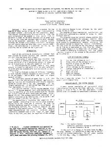
Fig. 1. Service areas of the transmitters of the primary network modeled as Voronoi polygons.

tence of primary and secondary networks. We then describe the used data sets and simulation models in Section III, together with a brief description of the developed simulation environment. The results from our study are then discussed in Sections IV and V, first focusing on occurrence of transmit opportunities and then on evaluating the utility of these transmit opportunities for the secondary network. In particular, we give extensive results on the distribution of achievable capacities in the secondary network and its dependence on the details of the scenario. Finally, we conclude the paper in Section VI. II. S YSTEM M ODEL AND A SSUMPTIONS We consider a collection of n primary user transmitters (usually corresponding to base stations or access points), the locations of which are represented by the vector X = {X1 , . . . , Xn } ∈ R2n . In order to develop a system model for secondary use around the transmitters X, we need to define protected areas for primary receivers outside which secondary use is possible with a given transmit power. Focusing on the downlink band, we first approximate the service area of a transmitter Xi ∈ X by its Voronoi polygon [20], [21]  V (Xi ) ≡ y ∈ R2 ky − Xi k ≤ ky − Xj k , j 6= i , (1) which consists of those points that are closer to Xi than any other transmitter (see Figure 1 for illustation). Since with typical radio technologies it is not possible to limit the actual coverage of the transmitter to the somewhat irregular shape of the Voronoi polygon, we consider the protected zone Z(Xi ) of an active transmitter Xi to consist of a disc centered at Xi and completely enclosing its service area represented by the Voronoi polygon V (Xi ). The use of Voronoi polygons is obviously an approximation, although quite reasonable one for many applications. The system model itself is also general

Fig. 2.

Protected zones around active PU transmitters.

enough to easily incorporate other definitions of the service areas without changes. For constructing the set of active transmitters, we consider both the time and frequency domains. We assume that the primary network has been allocated k channels, and assign the channels to the transmitters to minimize the aggregate downlink interference. Transmit powers are assigned to the primary network to guarantee a 95% coverage probability at the farthest corner of the service area of each transmitter (corresponding to the radius of the protected zone Z(Xi )), computed using a chosen propagation model. In the time domain, we assume that the activity pattern of each transmitter is represented by a stationary and ergodic ON/OFF process. Due to the diurnal cycle and daily variations, such processes would not be good approximations of actual transmitter activities over long time periods. However, they do provide accurate results assuming the durations of the individual ON and OFF periods and the timescale of temporal correlations between them are shorter than the period of the time the performance of the system is being analyzed over. These assumptions enable approximate modeling of most present-day technologies that use some variation of timedivision multiple access schemes, including, in particular, common OFDMA-based technologies such as WiMAX and LTE. However, especially in the latter case the OFF-periods would often have extremely short durations (on the order of individual time slots), and the actual usage of such spectrum holes might be very challenging technically. In such cases the results derived with the actual ON/OFF process will serve as (sometimes very loose) upper bounds on performance of secondary use. Limitations of the secondary user access mechanism can be incorporated into the analysis by considering instead a modified version of underlying ON/OFF process, obtained by removing OFF-periods that are shorter

360

than a given threshold which would depend on the sensing, scheduling and coordination techniques used. For example, OFF-periods corresponding to individual time slots could be removed, leaving only “session-level” ON/OFF patterns of the individual transmitters. The reader should also note that, for example, CDMA based wireless communication systems that tend to transmit continuously due to the presence of the broadcast channels are not well represented by this framework. The system model would also lose accuracy if the activity patterns of the transmitters would be highly correlated over the frequency band in question. Such additional refinements can, however, be included into the overall approach relatively easily. A special case of stationary and ergodic processes is the family of alternating renewal processes, for which the durations of active and inactive periods are assumed to be independent of each other but otherwise follow general distributions with mean values µon and µoff , respectively. Measurement studies have indicated that such models are realistic for a number of potential primary network technologies [22] and they are often used as models for performance evaluation of dynamic spectrum access systems. Let us assume that we observe the primary network at a time t which does not depend on the activity patterns of the transmitters. Then at time t each of them will be active with probability µon /(µon + µoff ) [23]. For most of our simulations we assume this probability to be the same for all transmitters, and call it the duty cycle of the primary network. In the more general case, the duty cycle would simply correspond to the probability of finding the transmitter active at any given time. Figure 2 illustrates the arising protected zones for the primary network of Figure 1 with three channels and duty cycle of 35%. In order to evaluate the utility of the spectrum holes arising in this framework we need to specify the model for primarysecondary coexistence. We adopt a model based on power control, in which the secondary user transmit power depends on its distance to the protected zones [24]–[26]. We first assume that the interference generated by the secondary user transmitting at power P for a primary network client at distance d away is given by I(dBm) = P (dBm) − L(d) + ξ,

(2)

where L(d) is the large-scale deterministic path loss and ξ is a normal random variable of mean zero used to model shadowing. Then the probability that this interference exceeds a threshold Imax becomes    Imax + L(d) − P 1 √ , (3) 1 − erf P {I ≥ Imax } = 2 σs 2 where σs is the standard deviation of ξ. We do not consider explicitly fast fading here, since usually it either can be averaged out in time domain, or the bandwidths of the technologies considered are large compared to the coherence bandwidth of the channels. However, adding it into the formalism is straightforward. We assume that the secondary nodes are allowed to transmit at a power that results in a bound ε on

this probability with respect to the point closest to them in the protected zones of the active transmitters (transmitting inside the protected zone of an active primary is not allowed as the interference towards a primary client cannot be bounded then). Equation (3) can be solved for P using this bound, yielding √ P (dBm) = Imax + L(d) + σ 2 erf −1 (2ε − 1) (4) for the allowed secondary transmit power. Figure 3 shows how this power depends on the location for the network configuration of Figure 2. We do not consider here explicitly the mechanisms secondary users should use to uncover these spectrum opportunities. Instead, we shall most of the time focus on studying the maximum, theoretically achievable capacity that assumes perfectly accurate determination of which transmitters are active. For realistic systems this would typically require explicit signaling between the primary and secondary networks, although mechanisms based on location information and measurements of aggregate transmit power, such as presented in [26], can be used as well provided the sensing time used is short enough compared to the active and inactive periods of the primary transmitters. It is clear that the reported results are much higher than what can be achieved with real systems. In our model the channels are very clean and we use maximum transmission power in the low duty cycle regions in which distances to nearest protected zones are large. In reality the expected capacities for secondary users would be considerably lower (as one would expect from the present day deployed systems). However, our results provide important capacity bounds and we have left the detailed study of the performance limitations induced by different implementation approaches for the secondary network for later work. Another property of realistic systems not explicitly considered here is the use of sectorization in dense primary network deployments. Including sectors into the modeling framework would somewhat increase the transmit opportunities for secondary users since the protected areas would further approach the service areas. Alternatively, one can consider a given duty cycle DCs for each of the k sectors, and consider the discs enclosing the service areas as protected zones if any of the sectors is active. If the activity patterns of the sectors are independent, the resulting overall primary network duty cycle with the above model would become 1 − (1 − DCs )k . For the large-scale deterministic path loss we adopt the XiaBertoni propagation model [27] defined for a given frequency f (expressed in GHz) and distance d (in kilometers) by L(d) = K + A1 log10 (f ) + A2 log10 (d) ,

(5)

where the constants K, A1 and A2 are taken to have values of 131.1 dB, 21 dB and 37.6 dB, respectively (see [28] for detailed discussion on the determination of these coefficients for the chosen propagation model). We assume the shadowing factor ξ to have zero mean, and standard deviation of σs = 7 dB. As mentioned above, these assumptions are also used to assign powers for the primary transmitters to yield a 95% coverage probability at the edge of the service area for a given receiver sensitivity θs . For most of our simulations we assume that

361

21 km

25 km

Fig. 3. Allowed transmit powers measured in dBm for the secondary user as given by equation (4) for the primary configuration shown in Figure 2.

1.45 km

2.3 km

Fig. 4. Node location data set obtained from the Vodafone network in downtown Barcelona.

θs = -107.5 dBm, a value similar to current cellular network technologies [29], but we also explore the influence of changes in this parameter on the results. The system model given above is rather general, enabling the study of metrics such as the distribution of allowed transmit powers and secondary network capacities over space, time and frequency for any given primary and secondary network configuration. In the next section we describe in detail the network configurations used in our study, together with the values of the different parameters used in simulations. We also note that this framework can easily be extended towards enabling a full study of temporal evolution of the said metrics by specifying the time model of the primary network activity more closely. However, for the present work, we believe that the focus on duty cycle as the key measure of the primary system activity enables useful conclusions to be drawn with significant level of generality. III. M ODELS FOR N ETWORK S TRUCTURE In order to apply the system model developed above, we need to specify locations of primary and secondary transmitters as well as the secondary clients. For this, we use both structures of various deployed networks as well as node location models based on those. For the primary network we

Fig. 5. Node location data set obtained from the T-Mobile network in Los Angeles.

use locations of base stations from cellular networks since they are a most representative example of a widely deployed non-broadcast system. Figures 4 and 5 show parts of the Vodafone network in Barcelona and the T-Mobile network in Los Angeles, both used extensively in the following. Of these, the Barcelona data set corresponds to a very dense urban deployment, whereas the Los Angeles data set is somewhat more sparser corresponding to a large suburb. For the secondary network we use stochastic node location models originally developed in [30]. These enable greater flexibility and realism than what can be obtained by assuming, for example, uniformly random deployment of nodes. The framework used in [30] specifies a probability density function for a collection of node locations in a region of interest, measuring how much more or less likely a given set of locations is to occur compared to the uniformly random case of unit density. In the reference it was established that the so-called Geyer saturation process [31] yields particularly versatile class of models, yielding good fits to both clustered network deployments (such as user-deployed femtocell networks), as well as regular, planned networks. The density function of the Geyer process is given by f (X) ∝ β #(X) γ sr,ζ (X) ,

(6)

where #(X) denotes the number of elements of X, sr,ζ (X) denotes the number of point pairs of X that are closer than distance r apart but each point being counted as part of at maximum ζ pairs, β > 0 controls the density of points, and γ ≥ 0 the nature of the process (clustered or regular). For example, if γ = 1 the Geyer model reduces to the uniformly random case, whereas if γ = 0 the process becomes a hardcore one, with no node pair being closer than distance r apart. The latter property can easily be seen directly from the density, which, if γ = 0, vanishes whenever sr,ζ (X) 6= 0. In [30] the model was fitted into various data sets, and based on these results the model parameters were chosen as given in Table I. The realizations of these models are illustrated in

362

TABLE I PARAMETERS FOR THE INSTANCES OF THE G EYER SATURATION MODEL USED IN THE SIMULATIONS . Parameters System type Dense urban secondary Suburban secondary Rural secondary Rural primary/cellular

r 150 250 3000 24000

ζ 2 2 2 2

β 10−5

3.3 × 6.0 × 10−7 3.0 × 10−8 1.6 × 10−8

γ 0.4112 1.6908 1.7995 0.5162

100 km

100 km

Fig. 7.

Fig. 6. Secondary nodes (represented by the small circles) with transmit opportunities obtained as a realization of the Geyer model for a Wi-Fi like dense hotspot network for the Barcelona scenario, together with the protected regions of the active primary transmitters.

Figure 6, showing a realization of the dense urban secondary case together with the protected regions generated using the Barcelona data set, and in Figure 7, depicting the rural cellular scenario also generated as a realization of the Geyer process. For computing capacities, we also need a model for the secondary user client locations. Assuming a scenario in which secondary transmitters act as access point or base stations, we distribute client locations from a bivariate normal distribution, with standard deviation of 15 m for urban scenarios, 85 m for suburban scenarios, and 1500 m for rural scenarios. A. Simulation Environment and Parameters All the simulations were carried out using a custom framework developed in the R environment [32], with the spatstat library [33] being used for some of the computations needed to implement the described system model and to generate realizations of the Geyer saturation process. For each combination of parameters up to 350 realizations of the scenarios were generated. Results were also analyzed by selecting random subsets to confirm that the obtained estimates for metrics of interest have low variance. The parameters of the propagation models were set to those given in Section II, and parameters of the node location models to those given above. The allowed interference probability was set to ε = 0.05, and interference threshold to Imax = -105 dBm. For the latter it is important to observer that the allowed secondary transmit power is linear in Imax , and thus results for other values can often be read from the graphs

Realization of the Geyer model for the rural cellular parameter set.

below by simply shifting the y-axis. The number of channels available to the primary network ranged in k ∈ {1, 3, 5, 7} corresponding to frequency reuse factors of 1, 1/3, 1/5 and 1/7, respectively. The operating central frequency was set to 2 GHz, but the results are not sensitive to small changes in the considered frequency band. For example, increasing the considered central frequency to 2.5 GHz would increase the allowed secondary transmit power by 2.03 dB. However, significant changes in the central frequency do have a major impact on results. For example, changing the central frequency to 700 MHz would reduce the transmit power of the secondary users by almost 10 dB under our system model. IV. I NFLUENCE OF THE P RIMARY N ETWORK ON S ECONDARY T RANSMIT O PPORTUNITIES We shall begin by studying the influence of the primary network structure and activity level on the distribution of allowed transmit powers of the secondary users. Figure 8 shows the distribution of the allowed transmit power for nodes with transmit opportunities, that is, for nodes outside the protected zones of active transmitters in the Barcelona scenario, assuming k = 3 channels being used by the primary network. We see that even in this very dense scenario the combination of frequency reuse and inactive periods in the primary network do leave residual transmit opportunities for the secondary network. However, with the exception of the very lowest duty cycles the allowed powers are very small, and not really suitable for applications beyond very short range communications. Figure 9 illustrates the allowed transmit power distribution for the case of the primary network for a higher frequency reuse factor of 1/5, showing that even increasing the spatial spectrum opportunities by making the set of primary transmitters operating on a given channel sparser does not yield significant increases in allowed powers in this scenario. The situation is significantly different in the suburban Los Angeles scenario as can be seen from Figure 10. The median

363

60 40 20

-60

-20

0

Allowed transmit power [dBm]

20 0 -20 -40

Allowed transmit power [dBm]

-80

0.1 0.1

0.3

0.5

0.7

0.3

0.5

0.7

0.9

Primary network duty cycle

0.9

Primary network duty cycle

0 -20 -40 -60

Allowed transmit power [dBm]

20

Fig. 8. The distribution of allowed transmit powers for different primary network duty cycles for the Barcelona scenario with frequency reuse factor of 1/3.

0.1

0.3

0.5

0.7

0.9

Primary network duty cycle

Fig. 9. The distribution of allowed transmit powers for different primary network duty cycles for the Barcelona scenario with frequency reuse factor of 1/5.

Fig. 10. The distribution of allowed transmit powers for different primary network duty cycles for the Los Angeles scenario with frequency reuse factor of 1/3.

of the allowed powers for the generated transmit opportunities is more than 1 W for low duty cycles, and even for high duty cycles around 20 dBm. However, as was also seen in the previous case, the variation in the allowed transmit powers is high, with inter-quartile range being around 20 dB for each of the duty cycles. This is due to the large variation in the distances of the secondary transmitters to their nearest protected zones. As can be expected, for the rural scenario even higher allowed transmit powers are obtained, as depicted in Figure 11. Even for 90% duty cycle the spatial opportunities induced by the frequency reuse and sparse infrastructure result in approximately 45 dBm allowed transmit powers with 50% probability for secondary nodes that are not in the protected zones. Most of the figures discussed above assumed a frequency reuse factor of 1/3. While this value is realistic for a number of conceivable application scenarios, it is clearly of interest to study more carefully the effects of higher and lower reuse factors. Figure 12 shows the distribution of the allowed transmit power for the Los Angeles scenario but, in contrast to Figure 10, without frequency reuse. For small duty cycles the transmit opportunities continue to be significant, but for higher duty cycle there is a reduction of approximately 10 dB in all the quartiles, as well as slightly increase variability. The main difficulty induced by high primary network duty cycle combined with the single-channel operation is, however, the significant reduction in the frequency of transmit opportunities. This is illustrated in Figure 13, showing the fraction of secondary network nodes that are able to transmit for various

364

60 20 0 -40

-20

Allowed transmit power [dBm]

40

80 60 40 20 0

Allowed transmit power [dBm]

0.1

0.3

0.5

0.7

0.9

0.1

Primary network duty cycle

0.3

0.5

0.7

0.9

Primary network duty cycle

Fig. 11. The distribution of allowed transmit powers for different primary network duty cycles for the rural scenario with frequency reuse factor of 1/3.

duty cycles and frequency reuse factors. We see that as the duty cycle is above 50% in the single channel case, only few percent of the secondary network nodes are allowed to transmit at all. For frequency reuse factor of 1/3, already one third of the secondary nodes can transmit even when the primary network duty cycle is 90%. Notice that while 70% blocking probability for the secondary access might sounds prohibitively high, this is for an individual channel. Assuming that n statistically identical channels in terms of transmit opportunities were available, the blocking probability of an arbitrarily chosen secondary would decay exponentially in the number of channels n. V. ACHIEVABLE C APACITIES IN S ECONDARY N ETWORKS We shall now move on from quantification of transmit opportunities to studying their utility for the secondary network. Our focus will be throughout this section on the secondary network downlink capacity, and how it depends on the primary network activity and structure. Since we are interested in understanding the performance the secondary network could achieve without focus on a particular technology, we take our metric to be the Shannon capacity C = B log2 (1 + SINR). For all of our scenarios the capacity results are dominated by interference from active primary transmitters, and neither noise or interference from other potentially active secondary transmitters has major influence for reasonable ranges of the corresponding parameters. This is a direct consequence of the adopted system model. Because of this we focus mostly on reporting the distribution of achievable downlink capacities without the contribution of secondary interference and in a

Fig. 12. The distribution of allowed transmit powers for different primary network duty cycles for the Los Angeles scenario with frequency reuse factor of 1.

normalized form (bit/s/Hz). However, we do illustrate through selected examples the influence of secondary network structure on results. Figure 14 shows the influence of the duty cycle on the achievable downlink capacity for the Barcelona scenario, assuming a frequency reuse factor of 1/3. For low duty cycles relatively high capacities can be achieved due to the long distances to nearest active primary transmitters, resulting in high transmit powers and SINR, but for higher duty cycles the achieved capacities are very small, despite the primary network performing frequency reuse. The major reason for this is the increased interference from the primary network as can be seen by the reduction of capacities even in the upper tail of corresponding capacity distribution. Slightly smaller contribution comes from downlinks between active secondary transmitters and clients situated nearby a secondary transmitter that does not have a transmit opportunity. However, this effect would not influence especially the upper quartile of the results since more than 25% of the secondary nodes have transmit opportunities. These results are comparable to those reported in [19], in particular regarding the scaling of achievable capacity as a function of the primary duty cycle. The actually capacities given there are lower roughly by a factor of two due to differences in the propagation model and assumptions on the secondary network structure, in particular the distances between secondary transmitters and receivers, but relationships between the capacities and primary network activity levels are very similar. Figure 15 shows the detailed behaviors of the downlink

365

0.6 0.4 0.2

Fraction of APs with transmit opportunities

0.6 0.4 0.2

Fraction of APs with transmit opportunities

0.8

0.8

0.7 0.6 0.5 0.4 0.3 0.2

Fraction of APs with transmit opportunities

0.3

0.5

0.7

0.9

0.0

0.0

0.1 0.0

0.1

0.1

Primary network duty cycle

0.3

0.5

0.7

0.9

0.1

Primary network duty cycle

0.3

0.5

0.7

0.9

Primary network duty cycle

0.4 0.3 0.2

Frequency

20 15

0.1

10 0

0.0

5

Achievable downlink capacity [ bps / Hz ]

25

0.5

30

Fig. 13. Number of nodes with transmit opportunities for different duty cycles for the Los Angeles scenario. Different graphs correspond to frequency reuse factors of 1 (left), 1/3 (middle) and 1/5 (right).

0.1

0.3

0.5

0.7

0.9

0

Primary network duty cycle

5

10

15

20

25

30

35

Achievable downlink capacity [ bps / Hz ]

Fig. 14. The achievable downlink capacity in terms of the Shannon limit in the secondary network for different primary network duty cycles for the Barcelona scenario with frequency reuse factor of 1/3.

Fig. 15. The distribution of achievable downlink capacities for the Barcelona scenario with frequency reuse factor of 1/3 and 30% primary network duty cycle.

capacity distribution for the Barcelona scenario with frequency reuse factor of 1/3 and assuming 30% duty cycle for the primary network. The concentration of probability around the origin arises from the problem of “long downlink” discussed above, caused by the lack of transmit opportunities for nearby secondary nodes. A practical system would in most scenarios again deal with such an occurrence through multi-channel operation (or simply through buffering if the application latency requirements are lax enough compared to the lengths of active periods), so the behavior of the upper tail of the

capacity distribution is on greater interest. From the figure we can see that most of the clients with an active nearby secondary transmitter benefit from significant downlink capacities, with median being well above 5 bps/Hz. Figure 16 shows similar capacity results with different duty cycles for the Los Angeles scenario, also for the case of primary network frequency reuse factor of 1/3. We see that the sparser structure of the primary network resulting the higher allowed transmit powers for the secondary nodes also translates to higher capacities compared to the Barcelona

366

0.6 0.3

0.5

0.12

0.3 0.2

0.2

Frequency

Frequency

0.4

0.10 0.08 0.06

Frequency

0.1

0.1

0.04

0.0 10

20

30

40

50

0.0

0.02 0.00 0

0

10

Achievable downlink capacity [ bps / Hz ]

20

30

40

0

Achievable downlink capacity [ bps / Hz ]

10

20

30

40

Achievable downlink capacity [ bps / Hz ]

30 25 20 15 0

0

5

10

Achievable downlink capacity [ bps / Hz ]

20 15 10 5

Achievable downlink capacity [ bps / Hz ]

25

Fig. 16. The distribution of achievable downlink capacities for the Los Angeles scenario with frequency reuse factor of 1/3. Different graphs correspond to primary network duty cycles of 10% (left), 30% (middle) and 50% (right).

0.1

0.3

0.5

0.7

0.9

0.1

Primary network duty cycle

0.3

0.5

0.7

0.9

Secondary network duty cycle

Fig. 17. The achievable downlink capacity in the secondary network for different primary network duty cycles for the rural scenario with frequency reuse factor of 1/3.

scenario. However, the increase is not as dramatic as might be expected. The key reason for this is the difference in the secondary deployment models. Recall that we assumed the distribution of secondary clients to be also sparser in the suburban Los Angeles case than in the Barcelona scenario. The resulting larger distances between the secondary transmitters and receivers reduce the benefits from higher allowed transmit powers by increasing the average path loss. This simple example highlights the need to consider carefully also the secondary user client deployment when estimating the expected

Fig. 18. The impact of intra-system interference for the capacity of the secondary network in the Barcelona scenario.

performance of a network based on dynamic spectrum access. Further confirmation can be seen in Figure 17, illustrating the capacity results for the rural scenario. Even though very high allowed transmit powers were observed, as shown in Figure 11, the actual secondary network performance in terms of capacity is worse than in the Barcelona scenario due to the sparsity of the secondary client distribution. All the above results have been for achievable capacity, that is, without considering the intra-system interference from other secondary transmitters. Figure 18 illustrates the influence of interference from other secondary transmitters on results, assum-

367

20 15 10 0

5

Achievable downlink capacity [ bps / Hz ]

25 20 15 10 5 0

Achievable downlink capacity [ bps / Hz ]

0.1

0.3

0.5

0.7

0.9

-112.5

Secondary network duty cycle

-107.5

-102.5

-97.5

-92.5

-87.5

-82.5

Sensitivity of the primary network client [ dBm ]

Fig. 19. The impact of intra-system interference for the capacity of the secondary network in the Barcelona scenario assuming clustered secondary system deployment.

ing a similar duty cycle model for the secondary transmitters as was done for the primary case. The results correspond to the lower primary network duty cycle considered, as in this case the secondary transmitters have most transmit opportunities and thus cause more intra-system interference. We see from the results that even if most of the secondary transmitters would be active simultaneously, the capacity limits would be reduced only by few bits/s/Hz compared to the ideal case. This is in part due to the small allowed transmit powers for the secondary users, illustrated in Figure 8 above, and the regular deployment model for the secondary network. If the structure of the secondary network is assumed to be less uniform, intra-system interference will play a more significant role. This is illustrated in Figure 19, obtained by assuming a clustered model for the secondary network transmitter locations. More precisely, locations of the clusters were chosen randomly in the region, and for each cluster the number of secondary transmitters was taken to follow the Poisson distribution with average of ten nodes. The coordinates of the nodes were then drawn from a two-dimensional normal distribution with standard deviation of 100 m. We can see from the figure that the performance degradation is more visible as secondary network duty cycle is increased, but significant opportunities for secondary use remain. We conclude this section by studying the influence of the primary user client sensitivity θs on the results. Figure 20 illustrates how changing θs influences the achievable secondary network capacity for the Barcelona scenario with 1/3 frequency reuse and primary duty cycle of 30%. We see that

Fig. 20. The influence of primary user client sensitivity on achievable secondary network downlink capacity for the Barcelona scenario with frequency reuse factor of 1/3 and primary network duty cycle of 30%.

the capacity distribution becomes more and more concentrated on lower values as θs is increased, that is, as the primary client is assumed to have lower and lower sensitivity. The reason for this is, of course, the increase in the primary network transmit power under our system model. Lower primary client sensitivity, i.e., higher θs , means that the primary transmitters need to utilize higher transmit powers to ensure the prescribed outage probability at the edge of the service area. Even with 30% duty cycle and having the primary network transmitters being distributed over three frequencies the residual increase in interference suffices to reduce the secondary capacity significantly. Figure 21 shows the same effect but assuming only 10% duty cycle for the primary network, resulting in significantly less severe degradation. It should be noted that these results were obtained keeping the value of Imax constant. In most systems the decreased primary client sensitivity would also mean higher tolerance to interference. Thus, especially in scenarios such as the femtocell case in which both primary and secondary network belong to the same stakeholder, Imax should be increased proportionally to allow also secondaries to transmit at higher powers and thereby maintain their SINR. VI. C ONCLUSIONS In this paper we have studied the performance of cognitive wireless networks with a focus on dynamic spectrum access. Using the developed system model we studied in detail the influence of the structure and dynamics of the primary network activity on the achievable performance of the secondary. The

368

ACKNOWLEDGMENT

20 15 10

R EFERENCES

0

5

Achievable downlink capacity [ bps / Hz ]

25

30

The authors would like to thank RWTH Aachen University and the German Research Foundation (Deutsche Forschungsgemeinschaft, DFG) for providing financial support through the UMIC research centre. We would also like to thank the European Union for providing partial funding of this work through the FARAMIR project (grant number ICT-248351). Finally, we thank the anonymous reviewers for their thoughtful comments which helped to significantly improve the quality of this paper.

-112.5

-107.5

-102.5

-97.5

-92.5

-87.5

-82.5

Sensitivity of the primary network client [ dBm ]

Fig. 21. The influence of primary user client sensitivity on achievable secondary network downlink capacity for the Barcelona scenario with frequency reuse factor of 1/3 and primary network duty cycle of 10%.

results show that dynamic spectrum access can yield significant capacities even in the presence of rather dense primary networks provided that the primary network is active at most 30–50% of the time. This indicates that utilizing dynamic spectrum access techniques in, for example, femtocells has potential to yield solutions of high spectral efficiency in areas in which the load on the primary network is moderate. However, our results also show that the capacity estimates depend strongly on a number of primary and secondary network characteristics, and that care should be applied when deriving such estimates for any particular application scenario. We also believe that the developed modeling framework is of independent interest. The combination of accurate statistical location models together with simple yet realistic models for derived characteristics such as service areas allows this approach to be used for a number of tasks related to performance evaluation of diverse wireless communication systems. These results obtained using real cell-tower locations are an important step forward in understanding the performance characteristics of secondary networks in scenarios in which the primary system consists of dynamic transmitters. As we have shown here, the details of the primary and secondary network structure and dynamics for different scenarios can change the capacity estimates even by an order of magnitude. We strongly advocate the use of well founded models for these, and in each case carrying out a proper sensitivity analysis in order to understand the impact of modeling assumptions on the obtained results.

[1] J. Mitola III and G. Maguire Jr, “Cognitive radio: making software radios more personal,” IEEE personal communications, vol. 6, no. 4, pp. 13–18, 1999. [2] Q. Zhao and B. Sadler, “A survey of dynamic spectrum access,” IEEE Signal Processing Magazine, vol. 24, no. 3, pp. 79–89, 2007. [3] S. Haykin, “Cognitive radio: brain-empowered wireless communications,” IEEE journal on selected areas in communications, vol. 23, no. 2, pp. 201–220, 2005. [4] I. F. Akyildiz, W.-Y. Lee, M. C. Vuran, and S. Mohanty, “Next generation/dynamic spectrum access/cognitive radio wireless networks: a survey,” Computer Networks: The International Journal of Computer and Telecommunications Networking, vol. 50, no. 13, pp. 2127 – 2159, 2006. [5] R. Tandra and A. Sahai, “SNR walls for signal detection,” IEEE Journal on Selected Topics in Signal Processing, vol. 2, no. 1, pp. 4–17, 2008. [6] T. Yucek and H. Arslan, “A survey of spectrum sensing algorithms for cognitive radio applications,” IEEE Communications Surveys & Tutorials, vol. 11, no. 1, pp. 116–130, 2009. [7] R. Tandra, M. Mishra, and A. Sahai, “What is a spectrum hole and what does it take to recognize one?” Proceedings of the IEEE, vol. 97, no. 5, pp. 824–848, 2009. [8] A. Ghasemi and E. S. Sousa, “Spectrum sensing in cognitive radio networks: the cooperation-processing tradeoff,” Wireless Communications and Mobile Computing, vol. 7, no. 9, pp. 1049–1060, 2007. [9] C. R. Stevenson, G. Chouinard, Z. Lei, W. Hu, S. J. Shellhammer, and W. Caldwell, “Ieee 802.22: The first cognitive radio wireless regional area network standard,” IEEE Communications Magazine, vol. 47, no. 1, pp. 130 –138, january 2009. [10] C. Cordeiro, K. Challapali, D. Birru, and S. Shankar, “Ieee 802.22: An introduction to the first wireless standard based on cognitive radios,” Journal of Communications, vol. 1, no. 1, pp. 38–47, April 2006. [11] A. Sahai, S. Mishra, R. Tandra, and K. Woyach, “Cognitive radios for spectrum sharing,” IEEE Signal Processing Magazine, vol. 26, no. 1, pp. 140–145, 2009. [12] K. Harrison, S. Mishra, and A. Sahai, “How much white-space capacity is there?” in New Frontiers in Dynamic Spectrum Access Networks, 2010. DySPAN 2010. 4th IEEE International Symposium on, 2010. [13] J. Lee, S. Lim, J. G. Andrews, and D. Hong, “Achievable transmission capacity of secondary system in cognitive radio networks,” IEEE International Conference on Communications, May 2010. [14] M. Vu, N. Devroye, and V. Tarokh, “An overview of scaling laws in ad hoc and cognitive radio networks,” Wireless Personal Communications, vol. 45, no. 3, pp. 343–354, 2008. [15] S. Srinivasa and S. Jafar, “Cognitive Radio Networks: How Much Spectrum Sharing is Optimal?” in IEEE Global Telecommunications Conference, 2007. GLOBECOM’07, 2007, pp. 3149–3153. [16] E. G. Larsson and M. Skoglund, “Cognitive radio in a frequencyplanned environment: some basic limits,” IEEE Transactions on Wireless Communications, vol. 7, no. 12, pp. 4800–4806, December 2008. [17] E. Larsson and M. Skoglund, “Cognitive radio in a frequency planned environment: Can it work?” in Global Telecommunications Conference, 2007. GLOBECOM ’07. IEEE, 2007, pp. 3548 –3552. [18] S. Panichpapiboon and J. Peha, “Providing secondary access to licensed spectrum through coordination,” Wireless Networks, vol. 14, pp. 295–307, 2008, 10.1007/s11276-006-9415-8. [Online]. Available: http://dx.doi.org/10.1007/s11276-006-9415-8

369

[19] R. Saruthirathanaworakun and J. Peha, “Dynamic primary-secondary spectrum sharing with cellular systems,” in Cognitive Radio Oriented Wireless Networks Communications (CROWNCOM), 2010 Proceedings of the Fifth International Conference on, 2010, pp. 1 –6. [20] A. Okabe, B. Boots, K. Sugihara, and S. Chiu, Spatial Tessellations: Concepts and Applications of Voronoi Diagrams, Probability and Statistics. Wiley, 2nd edition, 2000. [21] F. Aurenhammer, “Voronoi diagrams—a survey of a fundamental geometric data structure,” ACM Computing Surveys (CSUR), vol. 23, no. 3, pp. 345–405, 1991. [22] M. Wellens, J. Riihij¨arvi, and P. M¨ah¨onen, “Empirical time and frequency domain models of spectrum use,” Elsevier Physical Communication Journal, vol. 2, no. 1–2, pp. 10–32, March-June 2009. [23] U. Bhat and G. Miller, Elements of applied stochastic processes. Wiley New York, 1984. [24] M. Haddad, M. Debbah, and A. M. Hayar, “Distributed power allocation for cognitive radio,” in the 9th International Symposium on Signal Processing and Its Applications (ISSPA 2007), Feb. 2007, pp. 1–4. [25] Y. Yu, H. Murata, K. Yamamoto, and S. Yoshida, “Interference information based power control for cognitive radio with multi-hop cooperative sensing,” IEICE Transactions on Communications, vol. E91-B, no. 1, pp. 70–76, 2008. [26] J. Nasreddine, J. Riihij¨arvi, and P. M¨ah¨onen, “Location-based adaptive detection threshold for dynamic spectrum access,” in the 4th IEEE International Symposium on New Frontiers in Dynamic Spectrum Access Networks (DySPAN 2010), Singapore, April 2010. [27] L. Maciel, H. Bertoni, and H. Xia, “Unified approach to prediction of propagation over buildings for all ranges of base station antenna height,” IEEE transactions on vehicular technology, vol. 42, no. 1, pp. 41–45, 1993. [28] H. Xia, “A simplified analytical model for predicting path loss in urban and suburban environments,” IEEE Transactions on Vehicular Technology, vol. 46, no. 4, pp. 1040–1046, November 1997. [29] H. Holma and A. Toskala, WCDMA for UMTS: HSPA Evolution and LTE. wiley, 2010. [30] J. Riihij¨arvi and P. M¨ah¨onen, “Modeling Spatial Structure of Wireless Communication Networks,” in INFOCOM IEEE Conference on Computer Communications Workshops, 2010, 2010, pp. 1–6. [31] C. Geyer, “Likelihood inference for spatial point processes,” Stochastic Geometry: Likelihood and Computation, pp. 79–140, 1999. [32] R Development Core Team, R: A Language and Environment for Statistical Computing, R Foundation for Statistical Computing, Vienna, Austria, 2007, ISBN 3-900051-07-0. [Online]. Available: http://www.R-project.org [33] A. Baddeley and R. Turner, “Spatstat: an R package for analyzing spatial point patterns,” Journal of Statistical Software, vol. 12, no. 6, pp. 1–42, 2005, ISSN 1548-7660. [Online]. Available: www.jstatsoft.org

370