Inlier-based Outlier Detection via Direct Density Ratio Estimation Shohei Hido
Yuta Tsuboi Hisashi Kashima Tokyo Research Laboratory IBM Research, Japan { hido, yutat, hkashima } @jp.ibm.com
Masashi Sugiyama Department of Computer Science Tokyo Institute of Technology, Japan
[email protected]
Takafumi Kanamori Department of Computer Science and Mathematics Informatics Nagoya University, Japan
[email protected]
Abstract We propose a new statistical approach to the problem of inlier-based outlier detection, i.e., finding outliers in the test set based on the training set consisting only of inliers. Our key idea is to use the ratio of training and test data densities as an outlier score; we estimate the ratio directly in a semi-parametric fashion without going through density estimation. Thus our approach is expected to have better performance in high-dimensional problems. Furthermore, the applied algorithm for density ratio estimation is equipped with a natural cross-validation procedure, allowing us to objectively optimize the value of tuning parameters such as the regularization parameter and the kernel width. The algorithm offers a closed-form solution as well as a closedform formula for the leave-one-out error. Thanks to this, the proposed outlier detection method is computationally very efficient and is scalable to massive datasets. Simulations with benchmark and real-world datasets illustrate the usefulness of the proposed approach. Keywords: outlier detection, density ratio, importance
1
Introduction
The goal of outlier detection (a.k.a. anomaly detection, novelty detection, or one-class classification) is to find uncommon instances (‘outliers’) in a given dataset. Outlier detection is useful in various applications such as topic detection in news documents [14], intrusion detection in network systems [24], and defect detection from behavior patterns of industrial machines [3, 9]. For this reason, outlier detection has been studied thoroughly in statistics, machine learning, and data mining communities for decades [7]. A standard outlier detection problem falls into the cate-
gory of unsupervised learning due to lack of prior knowledge on the ‘anomalous data’. In contrast, the papers [4, 5] addressed a semi-supervised outlier detection problem where examples of outlier and inlier are available as a training set. The semi-supervised outlier detection methods could perform better than unsupervised methods thanks to additional label information, but such training samples are not always available in practice. Furthermore, the type of outliers may be diverse and thus the semi-supervised methods—learning from known types of outliers—are not necessarily useful in detecting unknown types of outliers. In this paper, we address a problem of inlier-based outlier detection where examples of inlier are available. More formally, the inlier-based outlier detection problem is to find outlier instances in the test set based on the training set consisting only of inlier instances. The setting of inlier-based outlier detection would be more practical than the semisupervised setting since inlier samples are often available abundantly. For example, in defect detection of industrial machines, we already know that there is no outlier (i.e., a defect) in the past since no failure has been observed in the machinery. Therefore, it is reasonable to separate the measurement data into a training set consisting only of inlier samples observed in the past and the test set consisting of recent samples from which we try to find outliers. As opposed to supervised learning, the outlier detection problem is vague and it is not possible to universally define what the outliers are. In this paper, we consider a statistical framework and regard instances with low probability densities as outliers. In light of inlier-based outlier detection, outliers may be identified via density estimation of inlier samples. However, density estimation is known to be a hard problem particularly in high dimensions, so outlier detection via density estimation may not work well in practice. To avoid density estimation, we may use One-class Sup-
port Vector Machine (OSVM) [19] or Support Vector Data Description (SVDD) [23], which finds an inlier region containing a certain fraction of training instances; samples outside the inlier region are regarded as outliers. However, these methods cannot make use of inlier information available in the inlier-based settings. Furthermore, the solutions of OSVM and SVDD depend heavily on the choice of tuning parameters (e.g., the Gaussian kernel width) and there seems to be no reasonable method to appropriately determine the values of the tuning parameters. To overcome the weakness of the existing methods, we propose a new approach to inlier-based outlier detection. Our key idea is not to directly model the training and test data densities, but only to estimate the ratio of training and test data densities in a semi-parametric fashion. Among existing methods of density ratio estimation [1, 8, 10, 16, 21, 22], we adopt an algorithm called unconstrained Least-Squares Importance Fitting (uLSIF) [10] for outlier detection. The reason for this choice is that uLSIF is equipped with a variant of cross-validation, so the values of tuning parameters such as the regularization parameter can be objectively determined without subjective trial and error. Furthermore, uLSIF-based outlier detection allows us to compute the outlier score just by solving a system of linear equations—the leave-one-out cross-validation error can also be computed analytically. Thus, the proposed method is computationally very efficient and therefore is scalable to massive datasets. Through experiments using benchmark datasets and a real-world dataset of failure detection in hard disk drives, our approach is shown to compare favorably with existing outlier detection methods and other density ratio estimation methods with higher scalability.
2
Outlier Detection via Direct Importance Estimation
In this section, we propose a new statistical approach to outlier detection. Suppose we have two sets of samples—training samples ntr te nte d {xtr j }j=1 and test samples {xi }i=1 in a domain D (⊂ R ). tr ntr The training samples {xj }j=1 are all inliers, while the test nte samples {xte i }i=1 can contain some outliers. The goal of outlier detection here is to identify outliers in the test set based on the training set consisting only of inliers. More formally, we want to assign a suitable inlier score for the test samples—the smaller the value of the inlier score is, the more plausible the sample is an outlier. Let us consider a statistical framework of the outlier dentr tection problem: suppose training samples {xtr j }j=1 are independent and identically distributed (i.i.d.) following a training data distribution with density ptr (x) and test samnte ples {xte i }i=1 are i.i.d. following a test data distribution
with strictly positive density pte (x). Within this statistical framework, test samples with low training data densities are regarded as outliers. However, ptr (x) is not accessible in practice and density estimation is known to be a hard problem. Therefore, merely using the training data density as an inlier score may not be promising in practice. In this paper, we propose using the ratio of training and test data densities, called the importance, as an inlier score: w(x) =
ptr (x) . pte (x)
If there exists no outlier sample in the test set (i.e., the training and test data densities are equivalent), the value of the importance is one. The importance value tends to be small in the regions where the training data density is low and the test data density is high. Thus samples with small importance values are plausible to be outliers. One may suspect that this importance-based approach is not suitable when there exist only a small number of outliers—since a small number of outliers cannot increase the values of pte (x) significantly. However, outliers are drawn from a region with small ptr (x) and therefore a small change in pte (x) significantly reduces the importance value. For example, let the increase of pte (x) be ϵ = 0.01; then 1 0.001 1+ϵ ≈ 1, but 0.001+ϵ ≪ 1. Thus the importance w(x) would be a suitable inlier score (see Section 4.3 for illustrative examples).
3
Direct Importance Estimation Methods
The values of the importance are unknown in practice, so we need to estimate them from the data samples. If we estimate the training and test densities from the data samples, it can suffer from the curse of dimensionality. So we would like to directly estimate the importance values without going through density estimation. In this section, we review such direct importance estimation methods which could be used for outlier detection.
3.1
Kernel Mean Matching (KMM)
The KMM method avoids density estimation and directly gives an estimate of the importance at training points [8]. The basic idea of KMM is to find w(x) b such that the mean discrepancy between nonlinearly transformed samples drawn from ptr (x) and pte (x) is minimized in a universal reproducing kernel Hilbert space [20]. The Gaussian kernel ¶ µ ∥x − x′ ∥2 (1) Kσ (x, x′ ) = exp − 2σ 2 is an example of kernels that induce a universal reproducing kernel Hilbert space. It has been shown that the solution
of the following optimization problem agrees with the true importance: °Z °2 Z ° ° ° min Kσ (x, ·)ptr (x)dx − Kσ (x, ·)w(x)pte (x)dx° ° w(x) ° F Z s.t. w(x)pte (x)dx = 1 and w(x) ≥ 0, where ∥ · ∥F denotes the norm in the Gaussian reproducing kernel Hilbert space. An empirical version of the above problem is reduced to the following quadratic program: nte nte X X 1 te wi wi′ Kσ (xte w i κi min i , x i′ ) − nte 2 ′ {wi }i=1 i=1 i,i =1 ¯n ¯ te ¯X ¯ ¯ ¯ wi − nte ¯ ≤ nte ϵ and 0 ≤ w1 , . . . , wnte ≤ B, s.t. ¯ ¯ ¯ i=1
where κi =
ntr nte X tr Kσ (xte i , xj ). ntr j=1
σ (≥ 0), B (≥ 0), and ϵ (≥ 0) are tuning parameters. The te solution {w bi }ni=1 is an estimate of the importance at the test te nte points {xi }i=1 . Since KMM does not require the density estimates, it is expected to work well. However, the performance of KMM is dependent on the tuning parameters B, ϵ, and σ and they cannot be simply optimized, e.g., by cross-validation since estimates of the importance are available only at the test points.
3.2
The LogReg classifier employs the following parametric model for expressing the conditional probability p(η|x): ( pb(η|x) =
Ã
1 + exp −η
m X
!)−1 ζℓ ϕℓ (x)
,
ℓ=1
where m is the number of basis functions and {ϕℓ (x)}m ℓ=1 are fixed basis functions. The parameter ζ is learned so that the negative regularized log-likelihood is minimized: "n à Ãm !! te X X te min log 1 + exp ζℓ ϕℓ (xi ) ζ
+
i=1 n tr X j=1
Ã
Ã
ℓ=1 m X
log 1 + exp −
!! tr
ζℓ ϕℓ (x )
# ⊤
+ λζ ζ .
ℓ=1
Since the above objective function is convex, the global optimal solution can be obtained by standard nonlinear optimization methods such as Newton’s method, conjugate gradient, and the BFGS method. Then the importance estimate is given by Ãm ! X w(x) b = exp ζℓ ϕℓ (x) . ℓ=1
An advantage of the LogReg method is that model selection (i.e., the choice of basis functions {ϕℓ (x)}m ℓ=1 as well as the regularization parameter λ) is possible by standard cross-validation since the learning problem involved above is a standard supervised classification problem.
3.3
Kullback-Leibler Importance Procedure (KLIEP)
Estimation
Logistic Regression (LogReg)
Another approach to directly estimating the importance is to use a probabilistic classifier. Let us assign a selector variable η = 1 to training samples and η = −1 to test samples, i.e., the training and test densities are written as ptr (x) = p(x|η = 1) and pte (x) = p(x|η = −1). Application of the Bayes theorem yields that the importance can be expressed in terms of η as follows [1]: w(x) ∝
p(η = 1|x) . p(η = −1|x)
The conditional probability p(η|x) could be approximated by discriminating test samples from training samples using a LogReg classifier, where η plays the role of a class variable. Below we briefly explain the LogReg method.
KLIEP [21, 22] also directly gives an estimate of the importance function without going through density estimation by matching the two distributions in terms of the KullbackLeibler divergence. Let us model the importance w(x) by the following linear model: b X w(x) b = αℓ φℓ (x), (2) ℓ=1
where {αℓ }bℓ=1 are parameters and {φℓ (x)}bℓ=1 are basis functions such that φℓ (x) ≥ 0 for all x ∈ D and for ℓ = 1, . . . , b. Then an estimate of the training data density ptr (x) is given by pbtr (x) = w(x)p b te (x). In KLIEP, the parameters α are determined so that the Kullback-Leibler divergence from ptr (x) to pbtr (x) is mini-
mized:
Z ptr (x) KL[ptr (x)∥b ptr (x)] = ptr (x) log dx w(x)p b te (x) Z Z ptr (x) dx − ptr (x) log w(x)dx. b (3) = ptr (x) log pte (x)
The first term is a constant, so it can be safely ignored. Since pbtr (x) (= w(x)p b te (x)) is a probability density function, it should satisfy Z Z 1 = pbtr (x)dx = w(x)p b (4) te (x)dx. The KLIEP optimization problem is given by replacing the expectations in Eqs. (3) and (4) with empirical averages: Ã b ! ntr X X max log αℓ φℓ (xtr j ) {αℓ }bℓ=1
s.t.
b X ℓ=1
j=1
αℓ
Ãn te X
ℓ=1
φℓ (xte i )
!
nte ntr X 1 X te b c= 1 H φ(xte φ(xtr i )φ(xi ) and h = j ). nte i=1 ntr j=1
e is given λα⊤ α is a regularization term. The solution α analytically by b c + λI b )−1 h, e = (H α where I b is the b-dimensional identity matrix. Since elee could be negative, it is modified as ments of α b = max(0b , α), e α where 0b is b-dimensional vector with all zeros. This is the solution of uLSIF, which can be computed analytically. Let us consider the leave-one-out cross-validation (LOOCV) score of uLSIF: ¸ nte · ³ ´2 1 X 1 te ⊤ (i) tr ⊤ (i) bλ bλ , φ(xi ) α − φ(xi ) α nte i=1 2
= nte and α1 , . . . , αb ≥ 0.
i=1
This is a convex optimization problem and the global solution—which tends to be sparse—can be obtained, e.g., by simply performing gradient ascent and feasibility satisfaction iteratively. See [16] for the convergence proof. Model selection of KLIEP is possible by a variant of likelihood cross-validation (LCV) [6] as follows. We first dintr vide the training samples {xtr j }j=1 into a training part and a validation part, the model is trained based on the training part, and then its likelihood is verified using the validation part; the model with the largest estimated likelihood is chosen. Note that this LCV procedure corresponds to choosing the model with the smallest KL[ptr (x)∥b ptr (x)].
3.4
where, for φ(x) = (φ1 (x), . . . , φb (x))⊤ ,
(i)
tr b λ is a parameter learned without xte where α i and xi . By (i) bλ using the well-known Woodbury inversion formula, α can be expressed as ( µ ¶ ⊤ (nte − 1)ntr φ(xte (i) i ) a b λ =max 0b , α a+ a te ⊤ nte (ntr − 1) nte − φ(xte i ) ate µ ¶) ⊤ ) a (nte − 1) φ(xte tr i , − atr + ate ⊤ nte (ntr − 1) nte − φ(xte i ) ate
where b a = A−1 h,
Unconstrained Least-Squares Importance Fitting (uLSIF)
ate = A−1 φ(xte i ),
atr = A−1 φ(xtr i ), In uLSIF, the linear importance model (2) is used and the parameters are determined so that the following objective function is minimized [10]: ¶2 Z µ 1 ptr (x) w(x) b − pte (x)dx 2 pte (x) Z Z Z 1 1 ptr (x)2 = w(x) b 2 pte (x)dx− w(x)p b (x)dx+ dx, tr 2 2 pte (x) where the last term in the right-hand side is a constant and therefore can be safely ignored. By the empirical approximation, the following optimization problem is obtained. · ¸ ⊤ 1 ⊤c ⊤ b e = argmin α Hα − h α + λα α , α 2 α
c + (nte − 1)λ I b . A=H nte
This expression implies that the matrix inverse needs to be computed only once (i.e., A−1 ) for computing the LOOCV score. Note that the size of A−1 is b × b, which is independent of the numbers of training and test samples. Thus LOOCV can be carried out very efficiently without repeating the hold-out loop.
4
Outlier Detection by uLSIF
In this section, we discuss the characteristics of importance estimation methods reviewed in the previous section and propose a practical outlier detection procedure based on uLSIF.
4.1
Discussions
For KMM, there is no objective model selection method. Therefore, model parameters such as the Gaussian width need to be determined by hand, which is highly subjective in outlier detection. On the other hand, LogReg and KLIEP give an estimate of the entire importance function. Therefore, the importance values at unseen points can be estimated and CV becomes available for model selection. However, LogReg and KLIEP are computationally rather expensive since non-linear optimization problems have to be solved. uLSIF inherits the preferable properties of LogReg and KLIEP. Furthermore, the solution of uLSIF can be computed analytically through matrix inversion and therefore uLSIF is computationally very efficient. Thanks to the availability of the closed-form solution, the LOOCV score can also be analytically computed without repeating the hold-out loop, which highly contributes to reducing the computation time in the model selection phase. Based on the above discussion, we decided to use uLSIF in our outlier detection procedure.
4.2
Heuristic of Basis Function Choice
In uLSIF, a good model may be chosen by LOOCV, given that a set of promising model candidates is prepared. Here we propose using a Gaussian kernel model centered at ntr the training points {xtr j }j=1 as model candidates, i.e., w(x) b =
ntr X
αℓ Kσ (x, xtr ℓ ),
ℓ=1 ′
where Kσ (x, x ) is the Gaussian kernel (1) with kernel width σ. ntr The reason why the training points {xtr j }j=1 are chonte sen as the Gaussian centers, not the test points {xte i }i=1 , is as follows. By definition, the importance w(x) tends to take large values if the training density ptr (x) is large and the test density pte (x) is small; conversely, w(x) tends to be small (i.e., close to zero) if ptr (x) is small and pte (x) is large. When a function is approximated by a Gaussian kernel model, many kernels may be needed in the region where the output of the target function is large; on the other hand, only a small number of kernels would be enough in the region where the output of the target function is close to zero. Following this heuristic, we decided to allocate many kernels at high training density regions, which can be achieved by setting the Gaussian centers at the training ntr points {xtr j }j=1 . Alternatively, we may locate (ntr + nte ) Gaussian kerntr te nte nels at both {xtr j }j=1 and {xi }i=1 . However, in our preliminary experiments, this did not further improve the performance, but just slightly increased the computational cost.
Since ntr is typically very large, just using all the training ntr points {xtr j }j=1 as Gaussian centers is already computationally rather demanding. To ease this problem, we practintr cally propose using a subset of {xtr j }j=1 as Gaussian centers for computational efficiency, i.e., w(x) b =
b X
αℓ Kσ (x, cℓ ),
ℓ=1
where cℓ is a template point randomly chosen from ntr {xtr j }j=1 . We use the above basis functions in LogReg, KLIEP, and uLSIF in the experiments.
4.3
Illustrative Examples
Here, we illustrate how uLSIF behaves in outlier detection. 4.3.1
Toy Dataset
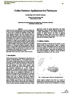
Let the dimension of the data domain be d = 1, and let the training density be (a) ptr (x) = N (x; 0, 1), (b) ptr (x) = 0.5N (x; −5, 1) + 0.5N (x; 5, 1), where N (x; µ, σ 2 ) denotes the Gaussian density with mean µ and variance σ 2 . We draw ntr = 300 training samples and 99 test samples from ptr (x), and we add an outlier sample at x = 5 for the case (a) and at x = 0 for the case (b) in the test set; thus the total number of test samples is nte = 100. The number of basis functions in uLSIF is fixed at b = 100, and the Gaussian width σ and the regularization parameter λ are chosen from a wide range of values based on LOOCV. The data densities as well as the importance values (i.e., the inlier scores) obtained by uLSIF are depicted in Figure 1. The graphs show that the outlier sample has the smallest inlier score among all samples and therefore the outlier can be successfully detected. Since the solution of uLSIF tends to be sparse, it may be natural to have a Gaussian-like curve as the inlier score (see Figure 1 again). 4.3.2
USPS Dataset
USPS is a dataset which contains images of hand-written digits provided by U.S. Postal Service. Each image consists of 256 (= 16 × 16) pixels, each of which takes a value between −1 to +1 representing its color in gray-scale. The class labels attached to the images are integers between 0 and 9 denoting the digits the images represent. Here, we try to find irregular samples in the USPS dataset by uLSIF. To the 256-dimensional image vectors, we append 10 additional dimensions indicating the true class to identify mislabeled images. In uLSIF, we set b = 100 and σ and λ are
∝ p tr(x) 1.2
uLSIF score True outlier
1.6
union of training and test samples as a test set: {xk }nk=1 = ntr te nte {xtr j }j=1 ∪ {xi }i=1 .
∝ p tr(x)
1.4
uLSIF score True outlier
1.2
1
5.1
1
0.8
Kernel Density Estimator (KDE)
0.8
0.6
KDE is a non-parametric technique to estimate a density p(x) from samples {xk }nk=1 . KDE with the Gaussian kernel is expressed as
0.6
0.4
0.4
0.2
0.2
0
0
−2
0
2
(a) N (x; 0, 1)
4
−5
0
(b) 12 (N (x; −5, 1)+N (x; 5, 1))
Figure 1. Illustration of uLSIF-based outlier detection.
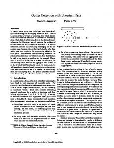
5 0 0 0 Figure 2. Outliers in the USPS test set.
0
4 3 2 3 9 Figure 3. Outliers in the USPS training set. chosen from a wide range of values based on LOOCV. Figure 2 shows the top 5 outlier samples in the original USPS test set (of size 2007) found by uLSIF where their original labels are attached next to the images. This result clearly shows that the proposed method successfully detects outlier samples that are very hard to recognize even by humans. We also consider an inverse scenario: we switch the training and test sets and examine the original USPS training set (of size 7291). Figure 3 depicts the top 5 outliers found by uLSIF, showing that they are relatively ‘good’ samples. This implies that the USPS training set consists only of high-quality samples.
5
pb(x) =
5
Relation to Existing Outlier Detection Methods
In this section, we discuss the relation between the proposed density-ratio based outlier detection approach with existing outlier detection methods. The outlier detection problem we are addressing in this nte paper is to find outliers in the test set {xte i }i=1 based on tr ntr the training set {xj }j=1 consisting only of inliers. On the other hand, the outlier detection problem that the existing methods reviewed here are solving is to find outliers in the test set without the training set. Thus the setting is slightly different. However, the existing methods can also be employed in our setting by simply using the
n X 1 Kσ (x, xk ), nte (2πσ 2 )d/2 k=1
where Kσ (x, x′ ) is the Gaussian kernel (1). The performance of KDE depends on the choice of the kernel width σ, but its value can be objectively determined based on LCV [6]: a subset of {xk }nk=1 is used for density estimation and the rest is used for estimating the likelihood of the held-out samples. Note that this LCV procedure corresponds to choosing σ such that the Kullback-Leibler divergence from p(x) to pb(x) is minimized. The estimated density values could be directly used as an inlier score. A variation of the KDE approach has been studied in the paper [11], where local outliers are detected from multi-modal datasets. However, density estimation is known to suffer from the curse of dimensionality, and therefore the KDE-based outlier detection method may not be reliable in practice1 . In our experiment, we will use a global KDE-based outlier detection method since we do not assume the multi-modality of the datasets.
5.2
One-class Support Vector Machine (OSVM)
SVM is one of the most successful classification algorithms in machine learning. The core idea of SVM is to separate samples in different classes by the maximum margin hyperplane in a kernel-induced feature space. OSVM is an extension of SVM to outlier detection [19]. The basic idea of OSVM is to separate data samples {xk }nk=1 into outliers and inliers by a hyperplane in a Gaussian reproducing kernel Hilbert space. More specifically, the solution of OSVM is given as the solution of the following quadratic programming problem: n 1 X wk wk′ Kσ (xk , xk′ ) {wk }k=1 2 ′
min n
k,k =1 n X
s.t.
k=1 1 The
wk = 1 and 0 ≤ w1 , . . . , wn ≤
1 , νn
density ratio can also be estimated by KDE, i.e., first estimating the training and test densities and then taking the ratio. However, the estimation error tends to be accumulated in this two-step process and our preliminary experiments showed that this is not useful.
where ν (0 ≤ ν ≤ 1) is the maximum fraction of outliers. OSVM inherits the concept of SVM, so it is expected to work well. However, the OSVM solution is dependent on the outlier ratio ν and the Gaussian kernel width σ; choosing these tuning parameter values could be highly subjective in unsupervised outlier detection. This is a critical limitation in practice. Furthermore, inlier scores cannot be directly obtained by OSVM; the distance from the separating hyperplane may be used as an inlier score, but its statistical meaning is rather unclear. A similar algorithm named Support Vector Data Description (SVDD) [23] is known to be equivalent to OSVM if the Gaussian kernel is used.
5.3
Local Outlier Factor (LOF)
The LOF is an outlier score suitable for detecting local outliers apart from dense regions [2]. The LOF value of an example x is defined using the ratio of the average distance from the nearest neighbors as LOFk (x) =
k 1 X lrdk (nearesti (x)) , k i=1 lrdk (x)
where nearesti (x) represents the i-th nearest neighbor of x and lrdk (x) denotes the inverse of the average distance from the k nearest neighbors of x. If x lies around a high density region and its nearest neighbor samples are close to each other in the high density region, lrdk (x) tends to become much smaller than lrdk (nearesti (x)) for every i. In such cases, LOFk (x) has a large value and x is regarded as a local outlier. Although the LOF values seem to be a suitable outlier measure, the performance strongly depends on the choice of the parameter k. To the best of our knowledge, there is no systematic method to select an appropriate value of k. In addition, the computational cost of the LOF scores is expensive since it involves a number of nearest neighbor search procedures.
5.4
Learning from Positive and Unlabeled data
A formulation called learning from positive and unlabeled data has been introduced in the paper [13]: given positive and unlabeled datasets, the goal is to detect positive samples contained in the unlabeled dataset. The assumption behind this formulation is that most of the unlabeled samples are negative (outlier) samples, which is different from the current outlier detection setup. In the paper [12], a modified formulation has been addressed in the context of text data analysis—the unlabeled dataset contains only a small number of negative documents. The key idea is to construct a single representative document of the negative
(outlier) class based on the difference between the distributions of positive and unlabeled documents. Though the problem setup is similar to ours, the method is specialized in text data, i.e., the bag-of-words expression. Since these above methods do not suit general inlierbased outlier detection scenarios, we will not include them in the experiments in Section 6.
5.5
Discussions
In summary, the proposed density-ratio based approach with direct density-ratio estimation would be more advantageous than KDE since it can avoid solving an unnecessarily difficult problem of density estimation. Compared with OSVM and LOF, the density-ratio based approach with LogReg, KLIEP, and uLSIF would be more useful since it is equipped with a model selection procedure. Furthermore, uLSIF is computationally more efficient than OSVM and LOF thanks to the analytic-form solution.
6
Experiments
In this section, we experimentally compare the performance of the proposed and existing algorithms. For all experiments, we used the standard statistical language environment R [17]. We implemented uLSIF, KLIEP, LogReg, KDE, and KMM by ourselves. uLSIF and KLIEP are implemented following the pseudo codes provided in the papers [10, 21, 22]. A package of the L-BFGS-B method called the optim is used in our LogReg implementation, and a quadratic program solver called the ipop contained in the kernlab package is used in our KMM implementation. We use the ksvm function contained in the kernlab package for OSVM and the lofactor function included in dprep package for LOF.
6.1
Benchmark Datasets
We use 12 datasets available from R¨atsch’s Benchmark Repository [18]. Note that they are originally binary classification datasets—here we regard the positive samples as inliers and the negative samples as outliers. All the negative samples are removed from the training set, i.e., the training set only contains inlier samples. In contrast, a fraction ρ of the negative samples are retained in the test set, i.e., the test set includes all inlier samples and some outliers. When evaluating the performance of outlier detection algorithms, it is important to take into account both the detection rate (the amount of true outliers an outlier detection algorithm can find) and the detection accuracy (the amount of true inliers that an outlier detection algorithm misjudges as outliers). Since there is a trade-off between the detection
rate and detection accuracy, we decided to adopt the Area Under the ROC Curve (AUC) as our error metric here. We compare the AUC values of the density-ratio based methods (KMM, LogReg, KLIEP, and uLSIF) and other methods (KDE, OSVM, and LOF). All the tuning parameters included in KDE, LogReg, KLIEP and uLSIF are chosen based on CV from a wide range of values. CV is not available to KMM, OSVM, and LOF; the Gaussian kernel width in KMM and OSVM is set as the median distance between samples, which has been shown to be a useful heuristic2 . The number of basis functions in uLSIF is fixed at b = 100. Note that b can also be optimized by CV, but our preliminary experimental results showed that the performance is not so sensitive to the choice of b and b = 100 seems to be a reasonable choice. For LOF, we test 3 different values for the number of nearest neighbors k. The AUC values as well as the normalized computation time are summarized in Table 1, showing that uLSIF and KLIEP work very well. Though the other methods perform well for some datasets, they also exhibit poor performance in other cases. On the other hand, the performance of uLSIF and KLIEP is relatively stable. In addition, from the viewpoint of computation time, uLSIF is much faster than KLIEP and other methods. Thus, the proposed uLSIFbased method could be a reliable and computationally efficient alternative to existing outlier detection methods.
6.2
Real-world Datasets
Finally, let us consider a real-world failure prediction problem in hard-disk drives equipped with the SelfMonitoring and Reporting Technology (SMART). The SMART system monitors individual drives and stores some attributes (e.g., the number of read errors) as time-series data. We use the SMART dataset provided by a manufacturer [15]. The dataset consists of 369 drives, where 178 drives are labeled as good and 191 drives are labeled as failed. Each drive stores up to the last 300 records that are logged almost every 2 hours. Although each record originally includes 59 attributes, we use only 25 variables chosen based on the feature selection test [15]. The sequence of records are converted into data samples in a sliding-window manner with window size ℓ. In practice, the training set may contain a few “bad” samples. To simulate such realistic situations, we construct the training set by choosing all records of the 178 good drives and adding a small fraction τ of ‘before-fail’ examples taken from the 191 failed drives which are more than 300 hours prior to failure. The test set is made of the records of the good drives and the records of the 191 failed drives 2 We experimentally confirmed that this heuristic works reasonably well in the current experiments.
less than 100 hours prior to failure; the “fail” samples are regarded as outliers in this experiment. First, we perform experiments for the window size ℓ = 5, 10 and evaluate the dependence of the feature dimension on the outlier detection performance. The fraction τ of before-fail examples in the training set is fixed to 0.05. Other settings including the fraction ρ of outliers and b are the same as the previous experiments. The results are summarized in Table 2. Next, we change the fraction of beforefail examples in the training set as τ = 0.05, 0.1, 0.15, 0.2 and evaluate the effect of heterogeneousness of the training set on the outlier detection performance. The fraction ρ of outliers in the test set is fixed to 0.05 and the window size ℓ is fixed to 10. The results are summarized in Table 3. Overall, the density-ratio based methods work very well; among them, uLSIF has the lowest computational cost. The performance of OSVM tends to be degraded as the outlier fraction ρ increases and the performance of KDE rapidly gets worse as the feature dimension ℓ increases. LOF works very well if the number of nearest neighbors k is large. However, a good choice of k may be problem-dependent and there seems no systematic way to determine k appropriately. The computation of LOF is very slow due to extensive nearest neighbor search, and the performance of LOF tends to be degraded if the fraction τ of before-fail examples in the training set is increased. These results indicate that our algorithm using the density ratio is accurate and computationally efficient in realworld failure prediction tasks—in particular, the use of KLIEP and uLSIF seems promising.
7
Concluding Remarks
We cast the inlier-based outlier detection problem as a problem of estimating the ratio of probability densities (i.e., the importance), and proposed a practical outlier detection algorithm based on uLSIF. Our method is equipped with a model selection procedure, which allows us to obtain a purely objective solution. This is a highly valuable feature in ill-defined problems such as outlier detection. Furthermore, the proposed method is computationally very efficient and therefore useful in practice. Through extensive simulations with benchmark and real-world datasets, the usefulness of the proposed approach was demonstrated.
References [1] S. Bickel, M. Br¨uckner, and T. Scheffer. Discriminative learning for differing training and test distributions. In Proceedings of the 24th International Conference on Machine Learning, pages 81–88, 2007. [2] M. M. Breunig, H.-P. Kriegel, R. T. Ng, and J. Sander. LOF: Identifying density-based local outliers. In Proceedings of
Table 1. Mean AUC values over 20 trials for the benchmark datasets. Dataset Name ρ 0.01 banana 0.02 0.05 0.01 b-cancer 0.02 0.05 0.01 diabetes 0.02 0.05 0.01 f-solar 0.02 0.05 0.01 german 0.02 0.05 0.01 heart 0.02 0.05 0.01 satimage 0.02 0.05 0.01 splice 0.02 0.05 0.01 thyroid 0.02 0.05 0.01 titanic 0.02 0.05 0.01 twonorm 0.02 0.05 0.01 waveform 0.02 0.05 Average Comp. time
uLSIF (CV) 0.851 0.858 0.869 0.463 0.463 0.463 0.558 0.558 0.532 0.416 0.426 0.442 0.574 0.574 0.564 0.659 0.659 0.659 0.812 0.829 0.841 0.713 0.754 0.734 0.534 0.534 0.534 0.525 0.496 0.526 0.905 0.896 0.905 0.890 0.901 0.885 0.661 1.00
KLIEP (CV) 0.815 0.824 0.851 0.480 0.480 0.480 0.615 0.615 0.590 0.485 0.456 0.479 0.572 0.572 0.555 0.647 0.647 0.647 0.828 0.847 0.858 0.748 0.765 0.764 0.720 0.720 0.720 0.534 0.498 0.521 0.902 0.889 0.903 0.881 0.890 0.873 0.685 11.7
LogReg (CV) 0.447 0.428 0.435 0.627 0.627 0.627 0.599 0.599 0.636 0.438 0.432 0.432 0.556 0.556 0.540 0.833 0.833 0.833 0.600 0.632 0.715 0.368 0.343 0.377 0.745 0.745 0.745 0.602 0.659 0.644 0.161 0.197 0.396 0.243 0.181 0.236 0.530 5.35
the ACM SIGMOD International Conference on Management of Data, pages 93–104, 2000. [3] R. Fujimaki, T. Yairi, and K. Machida. An approach to spacecraft anomaly detection problem using kernel feature space. In Proceedings of the 11th ACM SIGKDD International Conference on Knowledge Discovery and Data Mining, pages 401–410, 2005. [4] J. Gao, H. Cheng, and P.-N. Tan. Semi-supervised outlier detection. In Proceedings of the 2006 ACM symposium on Applied Computing, pages 635–636, 2006.
KMM (med) 0.578 0.644 0.761 0.576 0.576 0.576 0.574 0.574 0.547 0.494 0.480 0.532 0.529 0.529 0.532 0.623 0.623 0.623 0.813 0.861 0.893 0.541 0.588 0.643 0.681 0.681 0.681 0.502 0.513 0.538 0.439 0.572 0.754 0.477 0.602 0.757 0.608 751
OSVM (med) 0.360 0.412 0.467 0.508 0.506 0.498 0.563 0.563 0.545 0.522 0.550 0.576 0.535 0.535 0.530 0.681 0.678 0.681 0.540 0.548 0.536 0.737 0.744 0.723 0.504 0.505 0.485 0.456 0.526 0.505 0.846 0.821 0.781 0.861 0.817 0.798 0.596 12.4
k=5 0.838 0.813 0.786 0.546 0.521 0.549 0.513 0.526 0.536 0.480 0.442 0.455 0.526 0.553 0.548 0.407 0.428 0.440 0.909 0.785 0.712 0.765 0.761 0.764 0.259 0.259 0.259 0.520 0.492 0.499 0.812 0.803 0.765 0.724 0.690 0.705 0.594
LOF k = 30 0.915 0.918 0.907 0.488 0.445 0.480 0.403 0.453 0.461 0.441 0.406 0.417 0.559 0.549 0.571 0.659 0.668 0.666 0.930 0.919 0.895 0.778 0.793 0.785 0.111 0.111 0.111 0.525 0.503 0.512 0.889 0.892 0.858 0.887 0.887 0.847 0.629 85.5
k = 50 0.919 0.920 0.909 0.463 0.428 0.452 0.390 0.434 0.447 0.385 0.343 0.370 0.552 0.544 0.555 0.739 0.746 0.749 0.896 0.880 0.868 0.768 0.783 0.777 0.071 0.071 0.071 0.525 0.503 0.512 0.897 0.901 0.874 0.889 0.890 0.874 0.622
KDE (CV) 0.934 0.927 0.923 0.400 0.400 0.400 0.425 0.425 0.435 0.378 0.374 0.346 0.561 0.561 0.547 0.638 0.638 0.638 0.916 0.898 0.892 0.845 0.848 0.849 0.256 0.256 0.256 0.461 0.472 0.433 0.875 0.858 0.807 0.861 0.861 0.831 0.623 8.70
[5] J. Gao, H. Chengy, and P.-N. Tan. A novel framework for incorporating labeled examples into anomaly detection. In Proceedings of the 2006 SIAM International Conference on Data Mining, pages 593–597, 2006. [6] W. H¨ardle, M. M¨uller, S. Sperlich, and A. Werwatz. Nonparametric and semiparametric models. Springer Series in Statistics, 2004. [7] V. Hodge and J. Austin. A survey of outlier detection methodologies. Artificial Intelligence Review, 22(2):85– 126, 2004.
Table 2. SMART dataset: mean AUC values when changing the window size ℓ and the outlier ratio ρ Dataset ρ 0.01 5 0.02 0.05 0.01 10 0.02 0.05 Average Comp. time ℓ
uLSIF (CV) 0.894 0.870 0.885 0.868 0.879 0.889 0.881 1.00
KLIEP (CV) 0.842 0.810 0.858 0.805 0.845 0.857 0.836 1.07
LogReg (CV) 0.851 0.862 0.888 0.827 0.852 0.856 0.856 3.11
KMM (med) 0.822 0.813 0.849 0.889 0.894 0.898 0.861 4.36
OSVM (med) 0.919 0.896 0.864 0.812 0.785 0.783 0.843 26.98
k=5 0.854 0.850 0.789 0.880 0.860 0.849 0.847
LOF k = 30 0.937 0.934 0.911 0.925 0.919 0.915 0.924 65.31
k = 50 0.933 0.928 0.923 0.920 0.917 0.916 0.923
KDE (CV) 0.918 0.892 0.883 0.557 0.546 0.619 0.736 2.19
Table 3. SMART dataset: mean AUC values when changing heterogeneousness τ (ρ = 0.05 and ℓ = 10) Dataset τ 0.05 0.10 0.15 0.20 Average Comp. time
uLSIF (CV) 0.889 0.885 0.868 0.870 0.878 1.00
KLIEP (CV) 0.857 0.856 0.814 0.815 0.836 1.19
LogReg (CV) 0.856 0.846 0.785 0.778 0.816 3.78
KMM (med) 0.898 0.890 0.886 0.872 0.887 5.68
[8] J. Huang, A. Smola, A. Gretton, K. Borgwardt, and B. Sch¨olkopf. Correcting sample selection bias by unlabeled data. In Advances in Neural Information Processing Systems, volume 19, 2007. [9] T. Id´e and H. Kashima. Eigenspace-based anomaly detection in computer systems. In Proceedings of the 10th ACM SIGKDD International Conference on Knowledge Discovery and Data Mining, pages 440–449, 2004. [10] T. Kanamori, S. Hido, and M. Sugiyama. Efficient direct density ratio estimation for non-stationarity adaptation and outlier detection. In Advances in Neural Information Processing Systems, 2009, to appear. [11] L. J. Latecki, A. Lazarevic, and D. Pokrajac. Outlier detection with kernel density functions. In Proceedings of the 5th International Conference on Machine Learning and Data Mining in Pattern Recognition, pages 61–75, 2007. [12] X. Li, B. Liu, and S.-K. Ng. Learning to identify unexpected instances in the test set. In Proceedings of the 20th International Joint Conference on Artificial Intelligence, pages 2802–2807, 2007. [13] B. Liu, Y. Dai, X. Li, W. S. Lee, and P. S. Yu. Building text classifiers using positive and unlabeled examples. In Proceedings of the 3rd IEEE International Conference on Data Mining, pages 179–186, 2003. [14] L. M. Manevitz and M. Yousef. One-class SVMs for document classification. Journal of Machine Learning Research, 2:139–154, 2002. [15] J. F. Murray, G. F. Hughes, and K. Kreutz-Delgado. Machine learning methods for predicting failures in hard drives: A multiple-instance application. Journal of Machine Learning Research, 6:783–816, 2005.
OSVM (med) 0.783 0.785 0.784 0.749 0.775 30.83
k=5 0.849 0.846 0.831 0.847 0.843
LOF k = 30 0.915 0.841 0.835 0.866 0.864 74.30
k = 50 0.916 0.914 0.899 0.838 0.892
KDE (CV) 0.619 0.618 0.536 0.540 0.578 2.76
[16] X. Nguyen, M. J. Wainwright, and M. I. Jordan. Estimating divergence functions and the likelihood ratio by penalized convex risk minimization. In Advances in Neural Information Processing Systems 20, pages 1089–1096, 2008. [17] R Development Core Team. R: A language and environment for statistical computing. R Foundation for Statistical Computing, 2005. [18] G. R¨atsch, T. Onoda, and K. R. M¨uller. Soft margins for AdaBoost. Machine Learning, 42(3):287–320, 2001. [19] B. Sch¨olkopf, J. C. Platt, J. Shawe-Taylor, A. J. Smola, and R. C. Williamson. Estimating the support of a highdimensional distribution. Neural Computation, 13(7):1443– 1471, 2001. [20] I. Steinwart. On the influence of the kernel on the consistency of support vector machines. Journal of Machine Learning Research, 2:67–93, 2001. [21] M. Sugiyama, S. Nakajima, H. Kashima, P. von B¨unau, and M. Kawanabe. Direct importance estimation with model selection and its application to covariate shift adaptation. In Advances in Neural Information Processing Systems 20, pages 1433–1440, 2008. [22] M. Sugiyama, T. Suzuki, S. Nakajima, H. Kashima, P. von B¨unau, and M. Kawanabe. Direct importance estimation for covariate shift adaptation. Annals of the Institute of Statistical Mathematics, 60(4), 2008. to appear. [23] D. M. J. Tax and R. P. W. Duin. Support vector data description. Machine Learning, 54(1):45–66, 2004. [24] K. Yamanishi, J.-I. Takeuchi, G. Williams, and P. Milne. Online unsupervised outlier detection using finite mixtures with discounting learning algorithms. Data Mining and Knowledge Discovery, 8(3):275–300, 2004.