Input feature selection for classification problems - Semantic Scholar

Kwak, N. and Choi, C.. Input Feature Selection for Classification Problems. IEEE Trans. Neural Networks, v. 13, no.1, 2002, p. 143-159. IEEE TRANSACTIONS ON NEURAL NETWORKS, VOL. 13, NO. 1, JANUARY 2002

143

Input Feature Selection for Classification Problems Nojun Kwak and Chong-Ho Choi, Member, IEEE

Abstract—Feature selection plays an important role in classifying systems such as neural networks (NNs). We use a set of attributes which are relevant, irrelevant or redundant and from the viewpoint of managing a dataset which can be huge, reducing the number of attributes by selecting only the relevant ones is desirable. In doing so, higher performances with lower computational effort is expected. In this paper, we propose two feature selection algorithms. The limitation of mutual information feature selector (MIFS) is analyzed and a method to overcome this limitation is studied. One of the proposed algorithms makes more considered use of mutual information between input attributes and output classes than the MIFS. What is demonstrated is that the proposed method can provide the performance of the ideal greedy selection algorithm when information is distributed uniformly. The computational load for this algorithm is nearly the same as that of MIFS. In addition, another feature selection algorithm using the Taguchi method is proposed. This is advanced as a solution to the question as to how to identify good features with as few experiments as possible. The proposed algorithms are applied to several classification problems and compared with MIFS. These two algorithms can be combined to complement each other’s limitations. The combined algorithm performed well in several experiments and should prove to be a useful method in selecting features for classification problems. Index Terms—Feature selection, mutual information, neural networks (NNs), orthogonal array, Taguchi method.

I. INTRODUCTION

F

EATURE selection plays an important role in classifying systems such as neural networks (NNs). For the purpose of classification problems, the classifying system has usually been implemented with rules using if-then clauses, which state the conditions of certain attributes and resulting rules [2], [3]. However, it has proven to be a difficult and time consuming method. From the viewpoint of managing large quantities of data, it would still be most useful if irrelevant or redundant attributes could be segregated from relevant and important ones, although the exact governing rules may not be known. In this case, the process of extracting useful information from a large dataset can be greatly facilitated. In this paper, the problem of selecting relevant attributes among the attributes available for the purpose of classification is dealt with. This problem of feature selection has been tackled by several researchers [1], [4]–[10]. One of the most popular methods

Manuscript received December 13, 1999; revised May 4, 2000 and February 21, 2001. This work was supported in part by the Brain Science and Engineering Program of Korea Ministry of Science and Technology and Brain Korea 21 program of Korea Ministry of Education. N. Kwak is with the School of Electrical Engineering, Seoul National University, Seoul 151-744, Korea. C.-H. Choi is with the School of Electrical Engineering, ERC-ACI and ASRI, Seoul National University, Seoul 151-744, Korea. Publisher Item Identifier S 1045-9227(02)00341-7.

for dealing with this problem is the principal component analysis (PCA) method [4]. This method transforms the existing attributes into new ones considered to be crucial in classification. However from the viewpoint of maintaining data, this method is not desirable, as it needs to process all the data when new data is added. The main drawback of this method is that it is not immune from distortion under transformation. Simply scaling some of the attributes can cause serious changes to the results. Recently, the feature selection problem has been dealt with intensely and some solutions have been proposed. One of the most important contributions has been made using the decision tree method. This uncovers relevant attributes one by one iteratively [9]–[12]. Setiono and Lui proposed a feature selection algorithm based on a decision tree by excluding the input features of the NN one by one and retraining the network repeatedly [9]. It has many attractive attributes but it basically requires the process of retraining for almost every combination of input features. To overcome this shortcoming, a fast training algorithm other than the backpropagation (BP) is used, but nevertheless requires a considerable amount of time. The classifier with dynamic pruning (CDP) of Agrawal et al. is also based on the decision tree which makes use of the mutual information between inputs and outputs [10]. It is very efficient in finding rules which map inputs to outputs but as a downside, requires a great deal of memory, because it generates and counts all the possible input–output pairs. Battiti’s mutual information feature selector (MIFS) [1] uses mutual information between inputs and outputs like the CDP. He demonstrated that mutual information can be very useful in feature selection problems and the MIFS can be used in any classifying systems for its simplicity whatever the learning algorithm may be. But the performance can be degraded as a result of large errors in estimating the mutual information. Regarding the topic of selecting appropriate number of features, stepwise regression [13] and Winston’s best-first search [14] are considered as a standard technique. The former uses a statistical partial F-test in deciding whether to add a new feature or to stop regression. The latter searches the space of attribute subsets by greedy hillclimbing augmented with backtracking facility. Since it does not care how the performance of subsets are evaluated, the sucess of the algorithm usually depends on the subset evaluation scheme. This paper investigates the limitation of MIFS using a simple example and proposes an algorithm which can overcome this limitation and improve performance. The Taguchi method [15], [16] to the feature selection problem is also applied. The Taguchi method was devised for robust design of complex systems and has been successfully applied in many manufacturing problems. Recently, Peterson et al. used the Taguchi method to find the NN structure that best fits the given data [17].

1045–9227/02$17.00 © 2002 IEEE

144

IEEE TRANSACTIONS ON NEURAL NETWORKS, VOL. 13, NO. 1, JANUARY 2002

In Section II, the basics of information theory and the Taguchi method are briefly presented with concepts such as entropy, mutual information, and orthogonal array. In Section III, the limitation of MIFS is analyzed and an improved version of MIFS is proposed. In Section IV, we show the limitation of the selection algorithms based on mutual information and how the Taguchi method can be incorporated in such cases. In Section V, the proposed algorithms are applied to several classification problems to show their effectiveness. And finally, conclusions follow in Section VI. In implementing classifying systems, we use NNs, but the proposed methods can be equally well used in other applications. II. PRELIMINARIES

Fig. 1.

In this section we briefly introduce some basic concepts and notations of the information theory and the Taguchi method which are used in the development of the proposed algorithms. A. Entropy and Mutual Information A classifying system such as NNs maps input features onto output classes. In this process, there are relevant features that have important information regarding output, whereas irrelevant ones contain little information regarding output. In solving feature selection problems, we try to find inputs that contain as much information about the output as possible and need tools for measuring the information. Fortunately, Shannon’s information theory provides a way to measure the information of random variables with entropy and mutual information [19], [20]. The entropy is a measure of uncertainty of random variables. If a discrete random variable has alphabets and the probaPr , , the bility density function (pdf) is entropy of is defined as

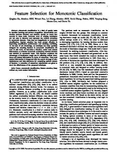
The relation between the mutual information and the entropy.

This, known as the “chain-rule,” implies that the total entropy and is the entropy of plus the reof random variables maining entropy of for a given . The information found commonly in two random variables is of importance in our work and this is defined as the mutual information between two variables (5) If the mutual information between two random variables is large (small), it means two variables are closely (not closely) related. If the mutual information becomes zero, the two random variables are totally unrelated or the two variables are independent. The mutual information and the entropy have the following relation, as shown in Fig. 1:

(1) is 2 and the unit of entropy is the bit. For two Here the base of , discrete random variables and with their joint pdf the joint entropy of and is defined as (2) When certain variables are known and others are not, the remaining uncertainty is measured by the conditional entropy

(6) Until now, definitions of the entropy and the mutual information of discrete random variables have been presented. For many classifying systems the output class can be represented with a discrete variable, while in general terms, the input features are continuous. For continuous random variables, though the differential entropy and mutual information are defined as

(7) (3) The joint entropy and the conditional entropy has the following relation:

(4)

) exit is practically impossible to find pdfs ( actly and to perform integration. Therefore we divide the continuous input feature space into several discrete partitions and calculate the entropy and mutual information using the definitions for discrete cases. The inherent error that exists in the process of conversion from continuous variables to discrete ones is bounded by some constant value which depends only on the number of partitions that divide the continuous space [21].

KWAK AND CHOI: INPUT FEATURE SELECTION FOR CLASSIFICATION PROBLEMS

145

B. The Taguchi Method The Taguchi method, based in part on the Fisher’s experimental methods [22], was applied for the robust design of products by Taguchi in the early 1950s. It developed in popularity first in Japan and later on in the U.S. and Europe [15], [16]. However, relatively few applications of this method in NNs exist [17]. Therefore we introduce this method in more detail. One basic ingredient of the Taguchi method is the orthogonal array (OA) which is used to find important control variables that influence the performance of a product among many candidate variables based on experiments and to assign them appropriate values. First, some control variables that are suspected of influencing the performance of a product are selected and then experiments are performed by changing the values of the control variables systematically. Then, the best combination of the values of the control variables are found. Suppose the experimental result can be represented as a , function of some discretized control variables . The purpose is to control these varii.e., ables and to make the result as close as possible to the desired value. If there are variables and for each control variable there are levels that can be changed, the full factorial method will disclose the best combination of the variables. However, to experiments. To reduce the time condo this, it requires sumed conducting experiments while taking advantage of the performance of the full factorial method, the orthogonal array method was introduced. It is a method of setting up experiments that only requires a fraction of the full factorial combinations. The treatment combinations are chosen to provide sufficient information to determine the factor effects. The orthogonal array ordains the order of experiments in a specific way. An example of the orthogonal array is shown in Table I. In Table I there are seven variables (A to G) and each variable has two levels (1,2). If we use the full factorial method to discover the optimal com) bination of variables, we need to experiment with 128 ( runs, whereas the orthogonal array allows us to experiment with only eight runs. The procedure of using the orthogonal array is quite simple. As shown in the table, in the first run, all the variables are set to level 1 and in the second run variables A to C are set to level 1 and variables D to G are set to level-2 and so on. We can compose numerous OAs by superimposing various Latin squares1 (see [18]) and generally, the OA is represented form. Here represents the number of runs to be in performed, is the number of levels of variables and is the number of variables. The OA in Table I is represented as or simply as . The way to construct an OA and some useful OAs can be found in [16]. In general, to determine the importance of a variable using the experimental results of OA, we use the analysis of the mean (ANOM) method [16]. It simply averages the results performed according to the OA to find the various factor effects. In the OA the orthogonality guarantees that all the levels are tested equally and the influences from other variables are assumed to be almost equal. Therefore the means of different levels of a variable are compared to determine the appropriate level of that variable. 1Each row and column of a Latin square has no duplicate element with equal sum.

TABLE I EXAMPLE OF THE OA

If the variation between the averages for different levels of a certain variable is small, it strongly suggestes that changing the level of that variable has little influence on performance and we can consider that it has a weak relation with the output. If the variation is large, we can assume that the variable influences the output greatly. The OA with ANOM performs ideally when the output can be represented as a linear combination of input variables. It also performs well when the interaction between variables is not so strong. It is widely recognized that if the output is roughly a monotonic function of each inputs, the OA with ANOM can still be successfully used to analyze the performance [16]. III. MUTUAL INFORMATION FEATURE SELECTOR UNDER UNIFORM INFORMATION DISTRIBUTION (MIFS-U) In this section a new algorithm for input feature selection using mutual information is presented. At first, the problem under consideration will be presented. A. The FR

Problem

In the process of selecting input features, it is desirable to reduce the number of input features by excluding irrelevant or redundant features among the ones that are extracted from raw data. This concept is formalized as selecting the most relevant features from a set of features and Battiti named it as a “feature reduction” problem [1]. ]: Given an initial set of features, find the subset [FR features that is “maximally informative” about the with class. As reviewed in the preceding section, the mutual information between two random variables measures the amount of information commonly found in these variables. The problem of selecting input features which contain the relevant information about the output can be solved by computing the mutual information between input features and output classes. If the mutual information between input features and output classes could be problem could be reformulated obtained accurately, the FR as follows. ]: Given an initial set with features and set [FR with features that of all output classes, find the subset , i.e., that maximizes the mutual information minimizes .

146

IEEE TRANSACTIONS ON NEURAL NETWORKS, VOL. 13, NO. 1, JANUARY 2002

Three key strategies for solving this FR problem can be presented for consideration. First, the “generate and test” are generated and their strategy. All the feature subsets are compared. Potentially, this can find the optimal subset but it is almost impossible due to the large number of combinations. Second, there is the “backward elimination” strategy. In this strategy, from the full feature set that contains elements, we eliminate the worst feature one-by-one until elements remain. This method also has many drawbacks in .2 The final strategy is “greedy selection.” computing In this method, starting from the empty set of selected features, we add the best available input feature to the selected feature set one by one until the size of the set reaches . This ideal greedy selection algorithm using mutual information is realized as follows. “initial set of features,” 1) (Initialization) set “empty set.” , 2) (Computation of the MI with the output class) . compute 3) (Selection of the first feature) find the feature that maxi, set , . mizes 4) (Greedy selection) repeat until desired number of features are selected. a) (Computation of the joint MI between variables) , compute . b) (Selection of the next feature) choose the feathat maximizes and set ture , . 5) Output the set containing the selected features. To compute the mutual information we must know the pdfs of variables, but this is difficult in practice, so the best we can do is to use a histogram of the data. In selecting features, if the output classes are composed of classes and we divide the th input feature space into parcells to titions to get the histogram, there must be . In this case, even for a simple problem of compute memories are needed selecting ten important features, if each feature space is divided into ten partitions. Therefore realization of the ideal greedy selection algorithm is practically impossible. To overcome this practical obstacle an alternative has to be devised. method of computing B. MIFS and its Limitation The MIFS algorithm is the same as the ideal greedy selection , algorithm except for Step 4. Instead of calculating the mutual information between a candidate for newly selected feature plus already selected features in and output classes and . To be selected, in , Battiti [1] used only a feature which cannot be predictable from the already selected features in , must be informative regarding the class. In the MIFS, Step 4 in ideal greedy selection algorithm was replaced as follows [1]:

j

2

2The number of memory cells needed to compute H (C S ) is K 5 P which can be very huge, where K is the number of classes, P is the number of partitions for ith input feature space and m is the number or elements in S

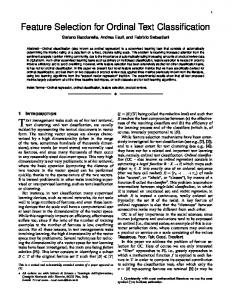
Fig. 2. The relation between input features and output classes.

4) (Greedy selection) repeat until desired number of features are selected. a) (Computation of the MI between variables) for all cou) with , , compute ples of variables ( , if it is not yet available. b) (Selection of the next feature) choose the feature that maximizes ; set , . Here is the redundancy parameter which is used in con, the sidering the redundancy among input features. If mutual information among input features is not taken into consideration and the algorithm selects features in the order of the mutual information between input features and output classes, the redundancy between input features is never reflected. As grows, the mutual informations between input features begin to influence the selection procedure and the redundancy becomes reduced. But in the case where is too large, the algorithm only considers the relation between inputs and does not reflect the input-output relation well. The relation between input features and output classes can be represented as shown in Fig. 2. The ideal greedy feature selection algorithm using the mutual information chooses the feature that maximizes joint mutual information which is the area 2, 3, and 4, represented by the dashed area in (area 2 and 4) is common for all the Fig. 2. Because unselected features in computing the joint mutual informa, the ideal greedy algorithm selects the feature tion that maximizes the area 3 in Fig. 2. On the other hand, the . MIFS selects the feature that maximizes , it corresponds to area 3 subtracted by area 1 in Fig. 2. For Therefore if a feature is closely related to the already selected feature , the area 1 in Fig. 2 is large and this can degrade the performance of MIFS. For this reason, the MIFS does not work well in nonlinear problems such as the following example. Example 1: Each of the random variables and is uniformly distributed on [ 0.5,0.5] and assume that there are three , and . The output belongs to class input features , if if When we take 1000 samples and partition each input feature space into ten, the mutual information between each input feature and the output classes and those between input features are ) shown in Table II. The order of selection by the MIFS ( , and in that order. is ,

KWAK AND CHOI: INPUT FEATURE SELECTION FOR CLASSIFICATION PROBLEMS

TABLE II FEATURE SELECTION BY MIFS FOR EXAMPLE 1

147

TABLE III VALIDATION OF (10) FOR EXAMPLE 1

Here corresponds to area 1 and 4 and corcorreresponds to area 1. So the term means the musponds to area 4 in Fig. 2. The term tual information between the already selected feature and the candidate feature for a given class . If conditioning by the and the class does not change the ratio of the entropy of mutual information between and , i.e., if the following relation holds: As shown in Table II(c) the MIFS selects rather than the as the second choice.3 more important feature This is due to the relatively large and is a good example showing a case where the relations between inputs are weighted too much. The MIFS handles redundancy at the expense of classifying performance.

(10) can be represented as (11)

C. Proposed Algorithm (MIFS-U) A feature selection algorithm that is closer to the ideal one than the MIFS is now proposed. The ideal greedy algorithm tries (area 2, 3, and 4 in Fig. 2) and this can to maximize be rewritten as (8) represents the remaining mutual information Here between the output class and the feature for a given . This is shown as area 3 in Fig. 2, whereas the area 2 plus area 4 repre. Since is common for all the candidate sents features to be selected in the ideal feature selection algorithm, there is no need to compute this. So the ideal greedy algorithm (area now tries to find the feature that maximizes requires as much 3 in Fig. 2). However, calculating . work as calculating with and So we will approximate , which are relatively easy to calculate. The conditional can be represented as mutual information (9)

Y

X

X0Y X0Y Z

3 can be calculated exactly by a linear combination of and . Because the output class can be computed exactly by and , we can say rather than is more informative about the for a given . We trained NNs and compared the classification rates later in Section V. As and are selected and 93.4% expected, the results are 99.8% when when and are selected.

X

X0Y

X

Y

Z

Y

X

X

X 0Y

Using the equation above and (9)

(12) If we assume that each region in Fig. 2 corresponds to its corresponding information, condition (10) is hard to satisfied when information is concentrated on one of the four regions in Fig. 2, , , , or . It is i.e., more likely that the condition (10) holds when information is in Fig. 2. distributed uniformly throughout the region of Because of this, we will refer to the algorithm, which will be proposed shortly, as the MIFS-U. We computed (10) for Example 1 and the values of several pieces of mutual information are shown in Table III. It shows that the relation (10) holds with less than 10% of error. With this formula, we revise Step 4) in the ideal greedy selection algorithm as follows: 4) (Greedy selection) repeat until desired number of features are selected. , compute if it a) (Computation of entropy) is not already available. b) (Computation of the MI between variables) for all cou) with , , compute ples of variables ( , if it is not yet available.

148

IEEE TRANSACTIONS ON NEURAL NETWORKS, VOL. 13, NO. 1, JANUARY 2002

c) (Selection feature

of

the

next feature) choose a that maximizes ; set , . can be computed in the process Here the entropy of computing the mutual information with output class , so there is little change in computational load with respect to the MIFS. In the calculation of mutual informations and entropies, there are two mainly used approaches of partitioning the continuous feature space: equidistance partitioning [1] and equiprobable partitioning [21]. In this paper, we used equiprobable partitioning method as in [1].4 Parameter offers flexibility to the algorithm as in the MIFS. If we set zero, the proposed algorithm chooses features in the order of the mutual information with the output. As grows, it excludes the redundant features more efficiently. In general we in compliance with (12). For all the experiments can set if there is no comment. to be discussed later we set , a second-order In computing mutual information joint probability distribution which can be computed from a and is required. Therefore, joint histogram of variables if there are features and each feature space is divided into partitions to get a histogram, we need memories for each of histograms to use MIFS-U. The computational effort thereas the number of features infore increases in the order of creases for given numbers of examples and partitions. This implies that MIFS-U can be applied to large problems without excessive computational efforts. IV. TAGUCHI METHOD IN FEATURE SELECTION Including the algorithm proposed in the previous section, the greedy algorithms using mutual information for input feature selection problems always select the feature that has the largest mutual information as the most important one. This method generally works well. However, if the algorithm selects a poor feature as the first candidate, the final feature set may give poor performance. This situation may occur if two or more combined features, instead of a dominant one, influence the classification procedure. To cope with this problem, we propose an algorithm using the Taguchi method which can be used together with the greedy algorithms described in the previous section. A. Limitation of the Greedy Selection Algorithms Using Mutual Information Consider the following example for the case where the greedy selection algorithms using mutual information does not work properly. and are Example 2: Each of the random variables uniformly distributed on [ 1,1] and assume that there are three . The output belongs to class input features , and if if 4If the distribution of the values in a variable f is not known a priori, we computed its mean  and standard deviation  and cut the interval [ ;   ] into p equally spaced segments. The points falling outside are assigned to the extreme left (right) segment.

2

02

+

ORDER

OF

SELECTION

FOR

TABLE IV EXAMPLE 2 USING GREEDY SELECTION ALGORITHMS

As can be seen, this is a variation of the typical XOR problem. When we take 1000 samples and partition each input feature space into ten, the mutual information between the input and the output as well as the order of selection using greedy algorithms are shown in Table IV. As in Table IV, both the MIFS and the MIFS-U select as the most important feature rather than or . This phenomenon occurs frequently when we employ the greedy selection algorithms with mutual information. This is difficult to avoid as long as only mutual information is used. In the following section, the Taguchi method is applied to deal with this kind of limitation. B. Input Feature Selection by the Taguchi Method In selecting input features, methods such as training NNs for many different combinations of input features can be contrived, in addition to the methods using mutual information. This kind of method such as Setiono’s [9], however, needs many different runs of training. To reduce the number of trainings, we adopt the orthogonal array as an input feature selection method, which is initially motivated from the idea of reducing the number of experiments in experimental design. The orthogonal array, as mentioned in Section II-B, is used to find the suboptimal solution by changing control variables (input features in this problem) systemically. To adopt the orthogonal array in selecting input features, we must first think of a way to determine the levels of each variable. The input feature selection problem can be considered as a problem of finding the combination of input features that perinput features and forms best in classification. If there are the levels of each input feature are determined by whether the feature is included in the feature set (level 1) or not (level 2), then there are two levels for each variable. Thus, there are different points in the search space and the optimal solution will be one of these points. The next issue to be considered is how close the solution obtained by the orthogonal array method can be to the optimal one. To obtain an optimal solution for this case, the output should be in the form of a linear combination of input features. This is unrealistic. In general, the Taguchi method provides better results when the interactions between control variables are relatively small. We can mitigate this condition if the output, with other input variables fixed, is a monotonic function of each input variable and in this case we can get quite good analysis on the system [16]. In the training of NNs, if a feature is a salient one, in general terms, the performance of training using it is supposed

KWAK AND CHOI: INPUT FEATURE SELECTION FOR CLASSIFICATION PROBLEMS

to be better than when it is not used. That is, for a given selected feature set, the inclusion of one of the remaining features would increase the performance of the classifying system if it were a salient one. Therefore, we can consider the output as a monotonic function of each salient feature, with other variables fixed. Consequently, if the orthogonal array is applied to this problem, good performance with a relatively small number of trainings can be expected. The following is a short explanation of how to apply the Taguchi method to the input feature selection problem (Table V). First we make an orthogonal array and let each column correspond to each input feature. Each row corresponds to one training of the NN with input features set to level 1 or level 2 in that row. After all of the rows are trained, we compare the average performance with a specific feature in the input vector and that without the feature. Then, we choose features which gives better average improvement in performance. In inputs, we need this algorithm when there are trainings.5 As we need experiments, we conclude that if we choose inputs in this way, we can get good input features with a relatively small number of trainings. The computational effort increases linearly with the number of features. Therefore the method can be applied with effect to large problems without excessive computational effort as in MIFS-U. A demonstration as to how to use the orthogonal array for the input feature selection problem will be given with the example of Table V. ) and we used the OA There are three input features ( as shown in Table V(a). of In Table V(b), the first row of OA represents that all the three features are selected as the input features. The NN with these features are trained to give 90% of the classification rate (in this case the performance measure is the classification rate). The second row of the table shows that the network trained solely gives 30% of the classification rate. In this way after all with the four trainings listed in the OA has been finished, the average performance using each feature and without it is calculated. For the average performance using this feature is example, for ) and that without it is 50% ( ) 60% ( and so on. With this average performance, the improvement of the average performance for each feature is evaluated. It is 10% , 20% for , while shows a 40% improvement. This for has the most influence on the performance of the means that network and can be regarded as the most salient feature. So we , , and in that order. selected features For most orthogonal arrays, the first row has a series of 1s and the others have 1s less than half the number of columns. If we use level 1 for the inclusion and level 2 for the exclusion of features, the training corresponding to the first row will always include all the features. Such an unbalance in the number of included features between the runs can degrade the performance of the selection procedure. To avoid this problem, we train the NN all over again with input vectors replacing level 1 (level 2) by level 2 (level 1) in Table V(b). With this additional training, we can select better features.

149

TABLE V EXAMPLE OF INPUT FEATURE SELECTION WITH OA

A relevant question to ask is what if there are hundreds of features that can make the size of OA extremely large. In such cases, we can use the Taguchi method after reducing the features by other selection algorithms such as the greedy selection algorithms described in the previous section and in doing so, better performance can be expected. The feature selection algorithm using the Taguchi method is summarized as follows: Taguchi Method in Feature Selection (TMFS) 1) (Filtering) If there are too many features, reduce the number of features to twice the number we want to select by using some algorithm such as the MIFS-U. 2) (Obtaining the orthogonal array) Obtain the orthogonal array corresponding to the number of features which are filtered in Step 1). . 3) Repeat the following steps with a) (Form an input feature vector for NN) For each row of the OA, form an input feature vector with features whose values are in the OA. b) (Training the NN) For each row, train the NN with the training data and store the performance for the test data. c) (ANOM) Calculate the average performance of each feature for its inclusion and exclusion in the input feature vector. Then, for each feature, evaluate the performance increment for its inclusion case over the exclusion case. 4) (Selecting the input features) For each feature, average and out the two increments in performance for cases in Step 3) and select input features by the order of these averaged terms. V. EXPERIMENTAL RESULTS

5d1e

within.

denotes smallest integer greater than or equal to the number enclosed

In this section we will present some experimental results which show the characteristics of the proposed algorithms.

150

In using the TMFS, to clarify the terminologies, we use the term “method I” when we compose the input feature set with elements corresponding to level 1 and “method II” for that with elements corresponding to level 2. The multilayer perceptrons (MLPs) used have one hidden layer and the BP algorithm is used to train the network. If the target value for an input pattern is 0 (1), the classification is assumed to be correct when the network’s output is below 0.3 (above 0.7). Otherwise, the classification is considered incorrect. In the training of NN, all the classification rates are for the test data except for the experiment A.3) and the meta-parameters of the NNs were set appropriately by performing several experiments. All the inputs were normalized on [0,1]. In the process of TMFS, we could have used different network structures as the number of features vary, but we kept them fixed because most number of features in each run is about half the number of columns for a given OA as described in Section II.

IEEE TRANSACTIONS ON NEURAL NETWORKS, VOL. 13, NO. 1, JANUARY 2002

COMPARISON

OF

MIFS

TABLE VI MIFS-U FOR EXAMPLE 1 (F 1 = X , ; F 1 AND F 2 ARE SALIENT FEATURES)

AND

F2 = X 0 Y , F3 = Y

TABLE VII ORDER OF SELECTION WHEN TMFS IS APPLIED TO THE EXAMPLE OF CASE 1

A. Simple Problems 1) MIFS-U Versus MIFS : For Example 1 in Section III-B, we compared the MIFS-U with the MIFS for several different values of and these results are shown in Table VI. The data consisted of 1000 patterns and the entropies and the mutual information are calculated by dividing each input feature space is a more important into ten partitions. To verify that ) and ( , ) feature than , we trained NNs with ( , as input features, respectively. The correct classification rates on the test data set were 99.8% for the first and 93.4% for the second network. The NNs were trained with sets of 200 training data and the classification rates are on the test data of 800 patterns. Two hidden nodes were used with a learning rate of 2.0 and momentum of 0.1. The number of epochs at the time of termination was 200. The result shows that when using the MIFS with as Battiti suggested [1], the results are unsatisfactory. The reason can be found in the characteristic of the problem. After the first selection of the feature that has the greatest mutual information with the output, the mutual information of other inputs with influences the selection of the second feature too much, as shown in Table II(c). The MIFS-U performs well for all values of including the suggested value 1. 2) TMFS Versus Greedy Selection Algorithms (Case 1) : For Example 2 in Section IV, we compared the greedy selection algorithms and the TMFS. The result of applying the TMFS to Example 2 is illustrated in Table VII. In each training of TMFS, the MLP has two hidden nodes, the learning rate and the momentum are 2.0, 0.1, respectively. We divided the data into sets of 200 training data and 800 test data. The number of training epochs was set to 300. One simulation was conducted for each row in Table VII to output TMFS result. From Table VII we select input features in the order of , and . As shown in Example 2 the greedy selection algorithms, like the MIFS and the MIFS-U, cannot select the correct input features in this problem, while the TMFS solves this problem correctly. 3) TMFS Versus Greedy Selection Algorithms (Case 2): The example we are going to consider was constructed by Elder [23]

as a counterexample to the CART [12], one of the greedy optimization algorithms. The dataset is given as follows [24]:

Here the output is a function of inputs , , and . As one can see from the data, the important features are and , because the . output can be exactly represented as The mutual information between each input feature and , , and , output are respectively. The MIFS and the MIFS-U select as the most is important feature, because the mutual information and . greater than

KWAK AND CHOI: INPUT FEATURE SELECTION FOR CLASSIFICATION PROBLEMS

151

TABLE VIII ORDER OF SELECTION WHEN TMFS IS APPLIED TO THE EXAMPLE OF CASE 2

TABLE IX ORDER OF SELECTION FOR MONK3 DATASET

When we apply the TMFS to this dataset, it identifies and as the salient features. The order of selected features is shown in Table VIII. The MLP has two hidden nodes and the learning rate and the momentum are 2.0 and 0.1, respectively. The terminating number of epochs was 200. One simulation was conducted for each row in Table VIII. In the training and testing, we used whole eight examples. 4) Monk3 Dataset : The monk3 dataset [25] is an artificial one in which robots are defined by different attributes. It has ) among binary classes and six discrete attributes ( which only the second, fourth, and fifth are relevant to the target where concept: and denote logical AND and OR, respectively. We used 1000 patterns in which the attributes are generated randomly and the output classes are decided according to the target concept. For a more realistic situation, we applied the feature selection algorithms to three monk3 datasets, where none, 5% and 10% of data are noise (misclassified), respectively. In the process of TMFS, we divided the data into 200 training data set and 800 test data set. The MLP has four hidden nodes as in [25] and the learning rate and the momentum are 0.01 and 0.9, respectively. The number of trainings was set to 10 000 epochs. One simulation was performed for TMFS. Filtering was orthogonal array was used. In Table IX we not used and a showed the result of feature selection. The bold faced features are relevant ones. The results show that the three algorithms performed well when the monk3 dataset had zero and 5% of noise. For cases with 10% of noise, the MIFS-U performed best while the MIFS last and the TMFS selected it fourth. selected

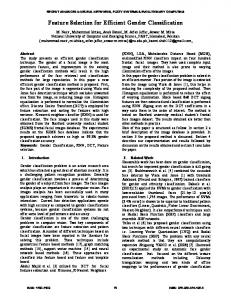
of the house, years house owned, and total amount of the loan. The three classification functions are shown in Table X. We generated 1000 input-output patterns and each input space was divided into ten partitions to compute the entropies and the mutual information. For convenience, we will refer to three datasets generated by using each function in Table X as IBM1, , reIBM2, IBM3, and nine input features as spectively. • MIFS-U Fig. 3 shows the mutual information between each input feature and the output classes for IBM1, IBM2, and IBM3, datasets. In Table XI, we compared the selected features by the MIFS-U , and the MIFS for the three datasets. For MIFS-U with the order of selection was exactly the same as the order of the mutual information with the output shown in Fig. 3. The features used in the classification functions are written in bold face in Table XI. As shown in Table XI, both the MIFS and the MIFS-U selected the desired features for the IBM1 and IBM2 datasets. , was selected as the eighth Note that for IBM2, when important one, while it was selected as the third for both the . This shows that both the MIFS and the MIFS-U with MIFS and the MIFS-U have the ability of effectively eliminating the redundant features. For IBM3 dataset the classification is determined by four features, i.e., salary( ), commission( ), elevel( ), and loan( ) as shown in Table X. So these four features must be chosen as salient features by good feature selectors. Table XI , , and in the first three shows that the MIFS selects is selected at the ninth with . This is an selection, but example of a case where too much weight is put on the mutual information between input features. As noted in Section III the method of excluding redundant features by MIFS may result in poor performance. For IBM3 we see that the MIFS-U selects the four features successfully. Table XII shows the selection results of IBM3 for various values of . Note the change in over in the MIFS case. Even the order of selection for as an for relatively small values of , the MIFS regards

B. IBM Datasets These datasets were generated by Agrawal et al.to test their [10] and Setiono et al.also used it data mining algorithm for testing the performance of their feature selector [9]. Each of the datasets has nine attributes, which are salary, commission, age, education level, make of the car, zipcode of the town, value

152

IEEE TRANSACTIONS ON NEURAL NETWORKS, VOL. 13, NO. 1, JANUARY 2002

TABLE X IBM CLASSIFICATION FUNCTIONS

(a) Fig. 3.

Mutual information between each feature and the output class for IBM datasets.

unimportant feature, while the MIFS-U does not. This shows that the MIFS-U performs consistently better than MIFS for different values of . • TMFS For IBM datasets we also tested the performance of the TMFS. To show the effectiveness of the filtering process, we compared the TMFS with and without the filtering process. . We For the filtering, we used the MIFS-U with filtered four and six features out of nine for IBM1 and IBM2,

respectively. An OA of was used for these datasets. We did not conduct the experiment with filtering step for IBM3 dataset, because the number of the relavant features are four whose double is close to the number of the full features. For all the experiments without the filtering step, we used an OA of . All the input features were assigned to the corresponding columns of the orthogonal array. The MLP has ten hidden nodes and the learning rate and the momentum are 0.01 and 0.9, respectively. The NNs were trained

KWAK AND CHOI: INPUT FEATURE SELECTION FOR CLASSIFICATION PROBLEMS

153

(b)

(c) Fig. 3. (Continued.) Mutual information between each feature and the output class for IBM datasets.

with 500 training data and the performances were evaluated on the remaining test data. The number of epochs in training is 10 000. One simulation is performed for each dataset. Table XIII shows the process of feature selection for the IBM1 dataset with full features. The last two columns in the table denote the classification rates on the test data set using method I and method II, respectively, and the second row from the last shows the difference in the average classification rate between the inclusion and the exclusion of each feature in the

input feature vector, namely the average improvement of the classification rate. The last row shows the order of selection. Fig. 4 shows the average improvement of the classification rates for each input feature by using the TMFS without filtering process. The features are selected by the order of the magnitude of the graph. We show the selection orders of TMFS with and without filtering process in the bottom of the Table XI. and are selected successfully. Also For IBM1 dataset , , , and are for IBM3, we can see that the features

154

TABLE XI FEATURE SELECTION FOR IBM DATASETS. THE BOLD FACED FEATURES ARE THE RELEVANT ONES IN THE CLASSIFICATION

selected successfully. In IBM2 dataset, the important features , , and , while the TMFS without filtering process are , , and . In Fig. 4 we see that is considered selects as the second least important feature. This result shows some resemblance to that of the greedy selection algorithm with (see Fig. 3). We can see in Table XI that this failure is resolved through the filtering process in the algorithm. We can say that the chance of selecting important features by the TMFS are high if the average improvement of correct classification for the input features are high. C. Sonar Target Dataset This dataset was constructed to discriminate between the sonar returns bounced off a metal cylinder and those bounced off a rock and it was used by Battiti to test the MIFSs performance [1]. The raw data is from UC-Irvine machine learning database [26]. It consists of 208 patterns including 104 training and testing patterns each. It has 60 input features and two output classes, metal/rock. As in [1], we normalized the input features to have the values in [0,1] and allotted one node per each output class for the classification. We divided each input feature space into ten partitions to calculate the entropies and mutual information. Unlike the IBM datasets, we do not know which features are important a priori, so we selected three

IEEE TRANSACTIONS ON NEURAL NETWORKS, VOL. 13, NO. 1, JANUARY 2002

TABLE XII ORDER OF FEATURE SELECTION FOR VARIOUS VALUES OF (IBM3)

to 12 features (top 5% to 20%) among the 60 features and trained the NN with the set of training patterns using these input features. We compared the classification rates of MIFS and MIFS-U. Then, we selected features by the TMFS. In the filtering process of the TMFS, we used both the MIFS and the MIFS-U and compared the results. Multilayer perceptrons with one hidden layer were used and the hidden layer had three nodes as in [1]. The conventional BP learning algorithm was used with the momentum of 0.0 and learning rate of 2.0. We trained the network for 300 epochs in all cases as Battiti did [1]. Fig. 5 shows the results of selection by the MIFS and the MIFS-U. In the figure, the x-axis denotes 60 features and the y-axis corresponds to the selection order. The feature that has a value of 60 is selected first, the feature with 59 is selected second, and so on. Using the TMFS, we also selected three to nine features from among twice the number of candidates produced through the for the filtering process. The orthogonal arrays used were for four, for six, and selection of three features, for nine, respectively. In Table XIV, we compare the performances of MIFS, MIFS-U, and TMFS filtered by either MIFS or MIFS-U for the test set. The classification rates for various numbers of selected features are compared. For comparison, we also conducted the stepwise regression [13] and best-first search algorithm [14] with correlation-based subset evaluator [27]. In the stepwise regression, we set confidence level to 0.1 and all the regression steps were set identical to those in [13]. It selected six features and the performance with these were 76.12%. The best-first algorithm reported 75.96% classification rate with 19

KWAK AND CHOI: INPUT FEATURE SELECTION FOR CLASSIFICATION PROBLEMS

155

TABLE XIII FEATURE SELECTION FOR IBM1 USING TMFS (L12 IS USED)

(a) Fig. 4. Average improvement of the classification rates for IBM datasets by TMFS.

features. In the table, all the resultant classification rates are the average values of ten experiments. In the table, we can see that the proposed algorithms produced better performances than the best-first algorithm with smaller number of features. In addition, the results show that the MIFS-U performed better than the MIFS by 10% in classification rate for the three to four selected features. In the other cases, the MIFS-U also worked better. In all cases, the TMFS performed better than the greedy algorithms used in the filtering process. The best performance was achieved when we used the TMFS filtered with the MIFS-U. In all the

cases, the TMFS/MIFS-U algorithm performed better than the TMFS/MIFS. To show the statistical significance of the improvements, we have performed the two-tailed T-test using Table XIV for the following four null hypotheses. • There is no difference between the performances of MIFS and MIFS-U. • There is no difference between the performances of MIFS and TMFS with MIFS. • There is no difference between the performances of MIFS-U and TMFS with MIFS-U.

156

IEEE TRANSACTIONS ON NEURAL NETWORKS, VOL. 13, NO. 1, JANUARY 2002

(b)

(c) Fig. 4. (Continued.) Average improvement of the classification rates for IBM datasets by TMFS.

• There is no difference between the performances of TMFS with MIFS and TMFS with MIFS-U. For each of the above hypotheses, the degree of freedom is , since the average is over ten experiments. For 18 degrees of freedom, the significance levels corresponding 1%, and 5%, are 2.878, and 2.101, respectively. The threshold ratio is computed as in Table XV. Since all the threshold ratios are well over 2.878, all the null hypotheses are rejected at the confidence level of 99%. Thus, we can say that MIFS-U is better

than MIFS, TMFS, with MIFS (MIFS-U) is better than MIFS (MIFS-U) and so on. This suggests that the combined TMFS and MIFS-U algorithm can be used effectively for feature selection problems. D. Ionosphere Dataset This Johns Hopkins University Ionosphere database [26] consists of 34 continuous valued attributes with a binary class. There are 351 instances and we compared the performance of

KWAK AND CHOI: INPUT FEATURE SELECTION FOR CLASSIFICATION PROBLEMS

157

(a)

(b) Fig. 5.

Order of selection for sonar dataset (MIFS and MIFS-U).

the proposed feature selection algorithms with the conventional MIFS with various s, best-first with correlation-based subset evaluator, stepwise regression and One-R feature selector [28]. In training the dataset, we used MLP with three hidden nodes, momentum of 0.1, learning rate of 1.0 and 300 terminating epochs. Table XVI is the result of the experiments. Among 34 features, we selected three to 20 features. Tenfold

cross validation was performed ten times for each experiments. The classification rates are the average of the ten experiments and standard deviations are provided in the parentheses. In performing TMFS, we preselected (filtered) 15 features with OA. MIFS-U and used In the table, we can see that the full 34 features do not produce best performance. Using MIFS-U or TMFS with MIFS-U, we

158

IEEE TRANSACTIONS ON NEURAL NETWORKS, VOL. 13, NO. 1, JANUARY 2002

(c) Fig. 5. (Continued.) Order of selection for sonar dataset (MIFS and MIFS-U). TABLE XIV CLASSIFICATION RATES WITH DIFFERENT NUMBERS OF FEATURES FOR SONAR DATASET (%) (THE NUMBERS IN THE PARENTHESES ARE THE STANDARD DEVIATIONS OF TEN EXPERIMENTS EACH)

TABLE XV THRESHOLD RATIO t FOR THE NULL HYPOTHESES

can get 3% to 4% performance improvement with only 10% of its features. The result shows the proposed algorithm performs better than the conventional feature selection methods especially when the small number of features are selected.

VI. CONCLUSION In this paper, we have proposed two input feature selection algorithms for classification problems. Algorithms, such as the MIFS, based on the information theory have strong advantages because they require relatively small computational effort.

KWAK AND CHOI: INPUT FEATURE SELECTION FOR CLASSIFICATION PROBLEMS

159

TABLE XVI CLASSIFICATION RATES WITH DIFFERENT NUMBERS OF FEATURES FOR IONOSPHERE DATASET (%) (THE NUMBERS IN THE PARENTHESES ARE THE STANDARD DEVIATIONS OF TEN EXPERIMENTS EACH)

But these algorithms handle redundancy at the expense of classifying performance. We have analyzed the limitations of the MIFS and proposed the MIFS-U for overcoming this limitation. The MIFS-U can provide the performance of the ideal greedy selection algorithm when the information is distributed uniformly and its computational complexity is almost the same as that of the MIFS. We have also applied the Taguchi method, which has been successfully used in many experimental design problems, to the feature selection problems and proposed the TMFS. Though it takes more computational effort than the algorithms based on the information theory, it can supplement the greedy selection algorithms. We have tested the TMFS with several examples and the results showed that it can be a valuable tool. When the number of input features are large, combining the MIFS-U with TMFS are expected to deliver a significant improvement in performance, especially when the number of selected input features has to be kept small. Because these methods do not require excessive computational effort, we can also apply these methods to large problems. We have used NNs as the classifying system, but these methods can be applied to other classifying systems as well. REFERENCES [1] R. Battiti, “Using mutual information for selecting features in supervised neural net learning,” IEEE Trans. Neural Networks, vol. 5, July 1994. [2] M.-S. Chen, J. Han, and P. S. Yu, “Data mining: An overview from a database perspective,” IEEE Trans. Knowledge Data Eng., vol. 8, Dec. 1996. [3] T. M. Anwar, H. W. Beck, and S. B. Navathe, “Knowledge mining by imprecise querying: A classification based approach,” in Proc. IEEE 8th Int. Conf. Data Eng., Phoenix, AZ, Feb. 1992. [4] I. T. Joliffe, Principal Component Analysis. New York: SpringerVerlag, 1986. [5] K. L. Priddy et al., “Bayesian selection of important features for feedforward neural networks,” Neurocomput., vol. 5, no. 2 and 3, 1993. [6] L. M. Belue and K. W. Bauer, “Methods of determining input features for multilayer perceptrons,” Neural Comput., vol. 7, no. 2, 1995. [7] J. M. Steppe, K. W. Bauer Jr., and S. K. Rogers, “Integrated feature and architecture selection,” IEEE Trans. Neural Networks, vol. 7, July 1996. [8] Q. Li and D. W. Tufts, “Principal feature classification,” IEEE Trans. Neural Networks, vol. 8, Jan. 1997. [9] R. Setiono and H. Liu, “Neural network feature selector,” IEEE Trans. Neural Networks, vol. 8, May 1997. [10] R. Agrawal, T. Imielinski, and A. Swami, “Database mining: A performance perspective,” IEEE Trans. Knowledge Data Eng., vol. 5, Dec. 1993. [11] R. Quinlan, C4.5: Programs for Machine Learning. San Mateo, CA: Morgan Kaufmann, 1993.

[12] L. Breiman, J. H. Friedman, R. A. Olshen, and C. J. Stone, Classification and Regression Trees. Belmont, CA: Wadsworth, 1984. [13] N. R. Draper and H. Smith, Applied Regression Analysis, 2nd ed. New York: Wiley, 1981. [14] P. H. Winston, Artificial Intelligence, MA: Addison-Wesley, 1992. [15] G. Taguchi, Taguchi on Robust Technology Development. New York: Amer. Soc. Mech. Eng., 1993. [16] W. Y. Fowlkes and C. M. Creveling, Engineering Methods for Robust Product Design. New York: Addison-Wesley, 1995. [17] G. E. P. Peterson et al., “Using Taguchi’s method of experimental design to control errors in layered perceptrons,” IEEE Trans. Neural Networks, vol. 6, July 1995. [18] [Online]. Available: http://www.research.att.com/~njas/oadir/ index.html [19] C. E. Shannon and W. Weaver, The Mathematical Theory of Communication. Urbana, IL: Univ. Illinois Press, 1949. [20] T. M. Cover and J. A. Thomas, Elements of Information Theory. New York: Wiley, 1991. [21] A. M. Fraser and H. L. Swinney, “Independent coordinates for strange attractors from mutual information,” Phys. Rev. A, vol. 33, no. 2, 1986. [22] R. A. Fisher, The Design of Experiments. Edinburgh, U.K.: Oliver and Boyd, 1935. [23] J. F. Elder, “Assisting inductive modeling through visualization,” in Joint Statistical Meeting, San Fransisco, CA, 1993. [24] V. S. Cherkassky and I. F. Mulier, Learning From Data. New York: Wiley, 1998, ch. 5. [25] S. B. Thrun et al., “The MONK’s problem—A performance comparison of different learning algorithms,” Dept. Comput. Sci., Carnegie Mellon Univ., Pittsburgh, PA, Tech. Rep. CMU-CS-91-197, 1991. [26] P. M. Murphy and D. W. Aha, UCI Repository of Machine Learning Databases, 1994. [27] M. A. Hall, “Correlation-Based Feature Subset Selection for Machine Learning,” Ph. D. dissertation, Univ. Waikato, Waikato, New Zealand, 1999. [28] G. Holmes and C. G. Nevill-Manning, “Feature selection via the discovery of simple classification rule,” in Proc. Int. Symp. Intell. Data Anal., Baden-Baden, Germany, 1995.

Nojun Kwak received the B.S. and M.S. degrees from the School of Electrical Engineering and Computer Science, Seoul National University, Seoul, Korea, in 1997 and 1999, respectively. He is currently pursuing the Ph.D. degree at Seoul National University. His research interests include neural networks, machine learning, data mining, image processing, and their applications.

Chong-Ho Choi (S’77–M’78) received the B.S. degree from Seoul National University, Seoul, Korea, in 1970 and the M.S. and Ph.D. degrees from the University of Florida, Gainesville, in 1975 and 1978, respectively. He was a Senior Researcher with the Korea Institute of Technology from 1978 to 1980. He is currently a Professor in the School of Electrical Engineering and Computer Science, Seoul National University. He is also affiliated with the Automation and Systems Research Institute, Seoul National University. His research interests include control theory and network control, neural networks, system identification, and their applications.