Journal of Clean Energy Technologies, Vol. 1, No. 4, October 2013
Input Partitioning Based on Correlation for Neural Network Learning Shujuan Guo, Sheng-Uei Guan, Shang Yang, Wei Fan Li, Lin Fan Zhao, and Jing Hao Song (0.1 or 0.05), it is considered that two variables is correlated to each other. To distinguish correlation level, the mean value of correlation of correlated attributes is calculated and employed as threshold. Any pair of correlated attributes whose correlation is greater than this threshold is considered to have strong correlation. Otherwise, it has weak correlation. The correlation coefficient table shows the correlation between input attributes. The diagonal element is the correlation between an attribute and itself and its value is always 1. The data on both sides of the diagonal is symmetric. For convenience, the table is converted to the form of lower triangular matrix.
Abstract—To improve the performance of neural network (NN), a new approach based on input space partitioning is introduced, i.e. partitioning according to the correlation between input attributes. As a result, the effect of weak correlation and non-correlation is excluded from the crucial stage of training. After partitioning, CBP network is introduced to train different sub-groups. The results from different networks are then integrated. According to the experimental results, improved performance is attained. Index Terms—Correlation, input attributes, neural network, partitioning.
I.
INTRODUCTION
Neural network (NN) is a supervised machine learning approach, which is often employed to solve classification problems. When solving classification problems with conventional NN, the input datasets often have multiple input attributes. Training these attributes together might not lead to the best performance. Sometimes, even poor results might be obtained. It is suggested that there exist positive or negative interaction between different attributes. If attributes with positive effect to each other were trained together, good performance might be attained. In this paper, we assume that the correlation between attributes is relevant to the degree of interaction. Although machine learning is the major approach for solving many practical problems, it has drawbacks such as low accuracy and weak generalization. To tackle these drawbacks, ensemble learning is introduced. It produces good generalization and accuracy by assembling multiple different models into one model, taking advantage of the difference between these models. In this paper, ensemble learning is employed to integrate the results of different sub-networks.
II.
Fig. 1. Input attribute sub-network model
III. CONSTRUCTIVE BACKPROPAGATION NEURAL NETWORK ALGORITHM Constructive Learning Algorithm consists of Dynamic Node Creation method [1], Cascade-Correlation [2] as well as its variations [3]-[5], Constructive Single-Hidden-Layer Network [6] and Constructive Back propagation [7] (CBP) and etc. For our work, CBP is used. IV. SUB-GROUPING MODEL OF INPUT ATTRIBUTE A. Input Attribute Grouping Model All of the input attributes are partitioned into r sub-groups with each sub-group containing at least one attribute:
CORRELATION
In statistics, correlation is defined as the strength and direction of linear relation in between the two random variables. There are several ways in calculating correlation. This paper employs Pearson correlation coefficients. We use P value and significant level (α) to identify whether two attributes are correlated to each other. If P < α
= =∑
) +∑
−
(
…+ = 1+ 2+…+ −1+1 (
Manuscript received January 2, 2013; revised February 23, 2013. This research is supported by the National Natural Science Foundation of China under Grant 61070085. Shujuan Guo, Sheng-Uei Guan and Shang Yang are with the School of Electronic & Information Engineering, Xi’an Jiaotong University, Xi’an, China (e-mail:
[email protected]) Weifan Li, Linfan Zhao and Jinghao Song are with the Dept. of Computer Science and Software Engineering, Xi’an Jiaotong-Liverpool University, Suzhou, China.
DOI: 10.7763/JOCET.2013.V1.76
∑
−
=∑ +…+∑
∑ ∑ +
+ ⋯+
∑
−
) +
)2 −
−
⋯
(
335
−
+∑
−
(
=
)
(1)
Journal of Clean Energy Technologies, Vol. 1, No. 4, October 2013
Especially, E1, E2,…Er are independent from each other. And the sum of them must be less than Eth.
B. Partitioning Algorithm of Input Features To improve the accuracy and efficient of neural network, the input attributes are grouped into several sub-groups. This strategy is designed to place together attributes that have strong correlation based on the basic situation that the input attributes are related to each other. Following is the algorithm description:
B. Sub-Network Model Sub-NN1, sub-NN2,…sub-NNr replace the original network after grouping. These sub-networks are trained by CBP network. The final result is generated by integrating the sub-networks by some ensemble learning method. V.
y List all input attributes pairs in descending order of correlation, group them in turns in this order. y For the two attributes in the same pair, if they weren’t grouped in any existing group, then form a new group with these two attributes. y If the two attributes all have been grouped already, then skip the pair. y If only one of the attributes has been grouped, the other one should be considered if it can be placed into the existing group in the prescribed order. If and only if an incoming attribute has strong correlation with all attributes in the group, it can be placed into this group. Once an attribute is assigned into a group, the other groups should not be considered. Otherwise form a new group for it. y After considering all with strong correlation, treat the remaining attributes as weak correlation with others.
PARTITIONING ALGORITHM BASED ON INPUT ATTRIBUTE
A. Definitions
Change of training time is a sensitive factor which effect CBP neural networks. On the one hand, if training is too short, neural network won’t be able to produce good result. On the other hand, long time training will result in overfitting and poor generalization with overmuch cost. This paper employs validation set to determine the training time [8], [9]. A dataset is divided into three sub dataset: a training set (50%) is used to train the network; a validation set (25%) is used to evaluate the quality of the network and avoid overfitting during the training; finally, a test set (25%) is used to evaluate the resultant network. The dependence on number of the coefficients in formula (1) and output values range can be reduced by using this E. Where, training error E is mean square error percentage [8] ∑
= 100
∑
(
−
)
We compare in the following the application results of this strategy with non-grouping. VI. ENSEMBLE LEARNING
(2)
Bagging [10] and Boosting [11] are most common ensemble learning methods in machine learning. Both Bagging and Boosting extract the training set to train when generate the sequence of predictive functions of sub-learner.. After generating the sequence of predictive functions, both algorithms use voting [12], [13] or weighted average method to integrate and generate the final predictive function. In this work, we adopt input space partitioning instead of training set partitioning. The input space is divided into several sub-sets with sub-learners respectively. Integration is similar to traditional ensemble learning method. In our approach, each sub-group only has a fraction of the original input space, it should be regarded as a relatively weak learner. According to the theory of ensemble learning, the integration of relatively weak learner often produces better result. Network ensemble method [14] is adopted in this paper.
In formula (2), omax and omin represent the maximum and minimum output values in formula (1). After epoch t, Etr (t) is average error of t times repeated trained network. Eva (t) is the corresponding error of validation set and it determines the time to stop training. Also, Ete (t) is the test error and the quality of the network will be evaluated by it. Eopt (t) represents the minimum validation error until epoch t. ( ) = min
(3)
( ′)
The relative increase of validation error over the minimum so far is defined as the generalization loss at epoch t: GL(t) = 100(
( ) ( )
(4)
− 1)
VII. EXPERIMENTAL RESULTS
Training will stop if generalization loss is too high. Otherwise, it will result in overfitting. A training strip of length m [8] is defined as the m times repeated sequence from n+1 to n+m. Especially, n must be divisible by m. During the training strip, Pm (t) measured the training progress. Pm (t) means the difference between average error and the minimum. ( ) = 1000(
∑ ∈
,… ∈
,…
( )
− 1)
UCI machine learning benchmarks are used. A. Diabetes From Table I, attribute relations can be illustrated in Table II. With Table II, sorting in order attribute pairs that are strongly correlated, and the result is: (1,8),(4,5),(4,6),(2,5),(2,6),(3,6),(3,4),(5,6). Applying the partitioning algorithm, we can get: {1,8}{4,5,6,7}{2}{3}. The experiment results are displayed in Tables III and IV.
(5)
336
Journal of Clean Energy Technologies, Vol. 1, No. 4, October 2013 TABLE VI: CANCER INPUT ATTRIBUTE RELATIONS TABLE Strong Correlation Weak Correlation Attribute
TABLE I: DIABETES INPUT ATTRIBUTE CORRELATION COEFFICIENTS TABLE
1
2,3
4,5,6,7,8,9
2
1,3,4,5,6,7,8
9
3
1,2,4,5,6,7,8
9
4
2,3,5,6,7
1,8,9
5
2,3,4,7
1,6,8,9
6
2,3,4,7
1,5,8,9
7
2,3,4,5,6,8
1,9
8
2,3,7
1,4,5,6,9
9
None
Strong correlation: Corrij> .583
B. Cancer From Table V, attribute relations can be illustrated in Table VI. Sorting in order attribute pairs with strong correlation, and the result is: (2,3), (2,7), (2,5), (3,7), (3,5), (3,4), (3,6), (2,8), (2,4), (3,8), (4,7), (6,7), (2,6),(1,3), (4,6), (1,2), (7,8), (4,5), (5,7). The grouping result obtained is: {2,3,7,5,4,9}{6}{8}{1}. The experimental results are presented in Tables VII and VIII.
*. Significantly correlated in level .05 (both sides). **. Significantly correlated in level .01 (both sides). Significantly correlated average: 246 TABLE II: DIABETES INPUT ATTRIBUTE RELATIONS TABLE
TABLE VII: LEARNING RESULTS FOR SUBGROUPS OF CANCER (Unit: %) Subgroup Classification Error {2,3,7,5,4,9} 3.4195 {6} 9.7701 {8} 9.1954 {1} 13.7931
Strong correlation: Corrij> .246 Wake correlation:Corrij< .246
TABLE VIII: EXPERIMENTAL RESULTS OF CANCER DATASET (Unit: %) Error Score Standard Improvement Solution Type Deviation Rate Mean Max Min Relational 1.2644 2.8736 0.5747 0.6876 32.31 grouping 0.6149 -----Non-grouping 1.8678 3.4483 1.1494
TABLE III: LEARNING RESULTS FOR SUBGROUPS OF DIABETES (Unit: %) Subgroup
Classification Error
{1,8} {4,5,6,7} {2}
29.9219 32.5781 23.5677
{3}
36.4583
1,2,3,4,5,6,7,8 Weak correlation: Corrij< .583
TABLE IX: GLASS INPUT ATTRIBUTE CORRELATION COEFFICIENTS TABLE TABLE IV: EXPERIMENTAL RESULTS OF DIABETES DATASET (Unit: %)
TABLE V: CANCER INPUT ATTRIBUTE CORRELATION COEFFICIENTS TABLE
*. Significantly correlated in level .05 (both sides). **. Significantly correlated in level .01 (both sides).Significantly correlated average: .354
C. Glass
From Table IX, attribute relations can be illustrated in Table X: Sorting in order attributes pairs that are strongly correlated, and the result is: (1,7), (4,8), (1,5), (3,4), (3,7), (4,6), (1,4), (2,8), (3,8). The grouping result obtained is: {1,7,9}{4,8,3}{5}{6}{2}. The experimental results are presented in tables XI and XII.
**. Significantly correlated in level .01 (both sides). Significantly correlated average: .583
337
Journal of Clean Energy Technologies, Vol. 1, No. 4, October 2013 TABLE X: GLASS INPUT ATTRIBUTE RELATIONS TABLE Attribute Strong Weak correlation Uncorrelated correlation s
space, the original network is divided into several sub-networks, each containing a fraction of the original input attributes and the whole output space. Every sub-network is trained by a CBP network, and then integrated by ensemble learning. From the experimental results, it can be inferred that this algorithm is effective upon the tested datasets. For further research, changing the ordering of attribute pairs can be considered to further enhance the performance.
1
4,5,7
2,6,8,9
3
2
8
1,3,6,7,9
4,5
3
4,7,8
2
1,5,6,9
4
1,3,6,8
7
2,5,9
5
1
6
2,3,4,7,8,9
6
4
1,2,5,7
3,8,9
7
1,3
2,4,6,9
5,8
8
2,3,4
1
5,6,7,9
[1]
9
None
1,2,7
3,4,5,6,8
[2]
REFERENCES
Strong correlation: Corrij> .354 Weak correlation: Corrij< .354 [3]
TABLE XI: LEARNING RESULTS FOR SUBGROUPS OF GLASS (Unit: %) Subgroup Classification Error {1,7,9} 49.5283 34.4340 {4,8,3} {5} 73.4906 {6} 63.0189 {2} 56.4151
[4] [5] [6] [7]
TABLE XII: EXPERIMENTAL RESULTS OF GLASS DATASET (Unit: %)
[8] [9] [10] [11]
D. Comparison of Experimental Results The final results compared with related work are shown in Table XIII: According to the table, the result of this experiment is fine. However, the generalization of the method has to be validated.
[12] [13] [14] [15]
TABLE XIII: COMPARISON OF RESULTS WITH DIFFERENT METHODS (Unit: %) Dataset Ang[16] ICNN Guan & Liu[15] 23.83 Diabetes 22.0313 22.8125 Cancer 1.2644 1.2069 -----Glass 30.7547 -----35.71
[16]
T. Ash, “Dynamic node creation in backpropagation networks,” Connection Sci., vol. 1, 1989, pp. 365–375. S. E. Fahlman and C. Lebiere, “The cascade-correlation learning architecture,” Advances in Neural Information Processing systems, vol. 2, 1990, San Mateo, CA: Morgan Kaufmann, pp. 524–532; L. Prechelt, “Investigation of the CasCor family of learning algorithms,” Neural Networks, vol. 10, 1997, pp. 85–896. S. Sjogaard, “Generalization in cascade-correlation networks,” in Proc. IEEE Signal Processing Workshop, 1992, pp. 59–68; S. U. Guan and S. Li, “An approach to parallel growing and training of neural networks,” in Proc. 2000 IEEE Int. Symp. Intell. Signal Processing Commun. Syst. (ISPACS2000), Honolulu, HI. D. Y. Yeung, “A neural network approach to constructive induction,” in Proc. 8th Int. Workshop Machine Learning, Evanston, IL, 1991. M. Lehtokangas, “Modeling with constructive backpropagation,” Neural Networks, vol. 12, 1999, pp. 707–716; L. Prechelt, A set of neural network benchmark problems and benchmarking rules, Technical Report 21/94, Department of Informatics, University of Karlsruhe, Germany, 1994. L. Rechelt, “Investigation of the CasCor family of learning algorithms,” Neural Networks, vol.10, no. 5, pp. 885–896, 1997. S. RE, “The strength of weak learnability,” Machine learning, 1990, vol. 5, no. 2, pp. 197-227. B. L. B. Predictors, Machine learning, vol. 24, no. 2, pp. 123-140, 1996, D. Bahler and L. Navarro, Methods for combining heterogeneous sets of classifiers, 2000. T. Dietterich, “Ensemble methods in machine learning,” Multiple classifier systems, 2000, pp. 1-15. M. H. Li, Based on the low interference the integration study method of neural network, Shanxi: Xi’an Jiaotong University, 2012. S. Guan and J. Liu, “Incremental Ordered,” Neural Network Training, vol. 12, 2002. J. Ang, S. Guan, K. Tan et al., “Interference-less neural network training,” Neurocomputing, vol. 71, no. 16-18, pp. 3509-3524, 2008. Sheng-Uei Guan received his M.Sc. & Ph.D. from the University of NorthCarolina at Chapel Hill. He is currently a professor in the computer scienceand software engineering department at Xi'an Jiaotong-Liverpool University(XJTLU). He is also affiliated with Xi’an Jiaotong University as an adjunctfaculty staff. Before joining XJTLU, he was a professor and chair inintelligent systems at Brunel
VIII. CONCLUSION This paper put forward an input space partitioning algorithm on the basis of sorting correlation among attribute pairs. It places attributes with significant correlation in subgroups in order to enhance the performance and precision of network learning. By partitioning the input
University, UK.
338