Inter-Cell Scheduling in Wireless Data Networks - CiteSeerX

Inter-Cell Scheduling in Wireless Data Networks Thomas Bonald† , Sem Borst?,‡ , Alexandre Prouti`ere† France Telecom R&D 38-40 rue du G´en´eral Leclerc, 92794 Issy-les-Moulineaux, France †

Bell Laboratories, Lucent Technologies P.O. Box 636, Murray Hill, NJ 07974-0636, USA ?

‡

CWI, P.O. Box 94079, 1090 GB Amsterdam, The Netherlands

Abstract: Over the past few years, the design and performance of channel-aware scheduling strategies have attracted huge interest. In the present paper we examine a different notion of scheduling, namely coordination of transmissions among base stations, which has received little attention so far. The inter-cell coordination comprises two key elements: (i) interference avoidance; and (ii) load balancing. The interference avoidance involves coordinating the activity phases of interfering base stations so as to increase transmission rates. The load balancing aims at diverting traffic from heavily-loaded cells to lightly-loaded cells. We consider a dynamic scenario where users come and go over time as governed by the arrival and completion of random data transfers, and evaluate the potential capacity gains from inter-cell coordination in terms of the maximum amount of traffic that can be supported for a given spatial traffic pattern. Numerical experiments demonstrate that inter-cell scheduling may provide significant capacity gains, the relative contribution from interference avoidance vs. load balancing depending on the configuration and the degree of load imbalance in the network.

1 Introduction Wireless networks are evolving to support a wide variety of high-speed data applications, in addition to conventional voice services and current low-bandwidth data services such as short messaging. Data applications tend to have drastically different traffic characteristics and QoS requirements than voice connections, calling for fundamentally different resource allocation mechanisms. In particular, wireless circuit-switched voice networks rely on power control algorithms for adjusting the transmit power so as to compensate for the varying channel quality and maintain a fixed transmission rate. Various data applications on the other hand, such as file transfers and Web browsing sessions, do not have a stringent rate requirement and are less sensitive to packetlevel delays. Such elastic applications are well-suited for rate control algorithms which adapt the transmission rate over time to track the fluctuations in the channel quality while transmitting at constant (maximum) power. Adaptive rate control mechanisms offer the possibility to improve the throughput performance by scheduling the data transmissions and exploiting the relative delay tolerance of data users. A particularly attractive approach, in fading environments, is to schedule the transmissions to the various users when their channel conditions are (relatively) favorable, as in the Proportional

Fair algorithm for the CDMA 1xEV-DO system [7, 17]. The design and performance of such channel-aware or opportunistic scheduling algorithms have been extensively studied over the past few years. Most of the studies have focused on the performance at the packet level for a static user population [2, 3, 18, 22, 23], although recently the flow-level performance in a dynamic setting has been analyzed as well [8, 13]. In the present paper we focus on a different notion of scheduling, namely coordination of transmissions among base stations (BS’s), which has received relatively little attention so far. The inter-cell scheduling that we consider comprises two key elements: (i) interference avoidance; and (ii) load balancing. The rationale for interference avoidance stems from the simple fact that the feasible transmission rates are impacted by the amount of interference from surrounding BS’s, so that significantly higher rates may be achieved when neighboring BS’s are switched off. When the increase in the feasible rates is sufficiently large, it may outweigh the sacrifice of transmission resources at the BS’s that are turned off, yielding a net benefit. The above observations are confirmed by the results in [6, 16, 19] which show that such inter-cell scheduling strategies achieve substantial throughput gains in a static scenario with a fixed ensemble of users. As mentioned above, inter-cell coordination is different in nature from opportunistic scheduling. However, the active control of interference is somewhat related in the sense that coordinating the activity phases of interfering BS’s may be interpreted as a form of network-wide opportunistic scheduling by generating favorable channel conditions in a coordinated fashion. Antenna-based incarnations of the latter concept (opportunistic beamforming to artificially induce channel variations) have been explored in [23]. The motivation for load balancing arises from the natural principle that the overall performance may be improved by diverting traffic from heavily-loaded BS’s to lightly-loaded BS’s. This may be achieved by allocating users to BS’s not solely on the basis of signal strength measurements, but taking load considerations into account as well, either average values or instantaneous conditions, see for instance [11, 15]. In the present paper we examine the potential capacity gains from inter-cell coordination in a situation where

users come and go over time as governed by the arrival and completion of random data transfers. Congestion manifests itself in this context by the number of active users competing for access to the transmission resources. In particular, the network may be unstable in the sense that the number of users may grow indefinitely. Thus we introduce as in [12] the notion of network capacity as the maximum amount of traffic compatible with stability for some given spatial traffic pattern. In other words, we focus on quantifying the capacity gains from inter-cell coordination so as to assess the potential benefit. The design of practical distributed scheduling schemes to realize these gains is left as a challenging topic for further research. In the subsequent analysis we focus on a scenario where each user is uniquely attached to a serving BS and each BS, when active, transmits to a single user. Such networks will be simply referred to as ‘TDMA networks’. Numerical experiments demonstrate that intercell scheduling may provide significant capacity gains in this practically interesting case, the relative contribution from interference avoidance vs. load balancing depending on the configuration and the degree of load imbalance in the network. The remainder of the paper is organized as follows. In Section 2 we present a detailed model description and in Section 3 we examine the stability region and introduce the notion of network capacity. These results are applied to ‘TDMA networks’ in Section 4. Section 5 is devoted to the numerical experiments and Section 6 concludes the paper.

2 Model description We consider the downlink of a network of BS’s N = {1, . . . , N } whose transmission resources (power, bandwidth, codes, etc) are shared by a dynamic population of data flows. Flows arrive at random and leave the network once the corresponding data transfer has been completed. Each flow is characterized by its size (in bits) and its data rate that depends on the user’s location, which is assumed to be fixed throughout the entire flow duration. Without loss of generality, we consider a set of classes I = {1, . . . , I} such that flows of any given class have the same size statistics and rate characteristics, as described below. 2.1 Traffic characteristics The traffic model is allowed to be very general. Classi flows arrive as a stationary ergodic process of intensity λi . Let σi be the mean size of class-i flows (in bits). The traffic intensity of class i is then defined by ρi = λi × σi (in bits/s). We denote by ρ = (ρ1 , . . . , ρI ) P the traffic intensity vector, by % = Ii=1 ρi the total traffic intensity, and by pi = ρi /% the proportion of the total traffic intensity generated by class i. Note that the traffic intensity % corresponds to the volume (in bits) that must be transmitted each second in the cell. 2.2 Resource allocation The service capabilities of the network are described by a set of available transmission ‘profiles’ J = {1, . . . , J}. Each of the profiles corresponds to a par-

ticular allocation of the transmission resources among the various classes. At any point in time, one of the available profiles can be selected for operating the network. When profile j is selected, the class-i flows share a data rate Ri,j , which is equal to zero when class i is not served in profile j. Evidently, the set of available profiles and the corresponding service rates strongly depend on the degree of flexibility in deploying the transmission resources. For now, however, we do not make any specific assumptions on the service rates, nor are we concerned how exactly the service rate of a class is shared among the active flows. When profile j is used a fraction ofP the time αj , the resulting service rate of class i is ri = j∈J αj Ri,j . The time allocation α = (α1 , . . . , αJ ) is termed the scheduling strategy. In the following, we P denote by T the set of non-negative vectors α such that j∈J αj = 1. When the time fractions are independent of the network state, the scheduling strategy is referred to as static. The strategy is called adaptive when the time fractions do depend on the network state. The set of achievable rate vectors r = (r1 , . . . , rI ) is referred to as the rate region:     X R = r : ∃α ∈ T , ∀i ∈ I, ri ≤ αj Ri,j .   j∈J

Remark 2.1 The above-described model falls in the general framework of queueing systems with interacting service resources [21, 4, 5, 20].

3 Stability region and network capacity We now determine the stability region of the network, i.e., the set of traffic intensity vectors ρ such that there exists a scheduling strategy for which the network is stable. Next, we will introduce the key notion of network capacity, defined for given traffic proportions of the classes (p1 , . . . , pI ) as the maximum traffic intensity % compatible with stability. The stability region has been characterized in [4]. It coincides with the interior of the rate region R. Proposition 3.1 There exists a scheduling strategy for ˘ with: which the network is stable if and only if ρ ∈ R,     X ˘ = r : ∃α ∈ T , ∀i ∈ I, ri < R αj Ri,j .   j∈J

The necessary condition follows trivially from the observation that the carried traffic vector must belong to the interior of the rate region. The sufficient condition read˘ then there exists ily follows from the fact that if ρ ∈P R, a time allocation α such that ρi < j∈J αj Ri,j for all i ∈ I. Under that static strategy, the network behaves as a set of I independent stable queues. We just observed that for any vector in the stability region there exists a static scheduling strategy α for which the network is stable. For any given static scheduling strategy α, on the other hand, the network P is stable if and only if ρi < ri for all i ∈ I, with ri = j∈J αj Ri,j .

The corresponding stability region is a strict subset of ˘ except in the trivial case where the set J reduces R, to a single transmission profile. Thus, static scheduling strategies are vulnerable and not necesarily desirable from a practical perspective. When the traffic proportions among classes (p1 , . . . , pI ) are fixed, however, there exists a unique static scheduling strategy α that stabilizes the network whenever possible. It is obtained by solving the linear program: X X minimize τj subject to τj ≥ 0, τj Ri,j ≥ pi . j∈J

j∈J

(1) The solution of this linear program τ ∗ corresponds to the minimum amount of time needed to transmit pi bits of class i, for all i ∈ I. Thus the maximum total traffic intensity is 1/τ ∗ , and the fraction of time that profile j is used is αj = τj∗ /τ ∗ . Given some fixed traffic proportions of the various classes (p1 , . . . , pI ), it is natural to define the network capacity as the maximum admissible total traffic intensity %, i.e., the maximum value of C such that the network is stable whenever % < C. By virtue of Proposition 3.1, the network capacity can be expressed as the optimal value of the following optimization problem: maximize C

subject to (p1 , . . . , pI )C ∈ R.

(2)

The optimal solution C ∗ is equal to 1/τ ∗ , where τ ∗ is the solution of the linear program (1). Thus evaluating the network capacity is equivalent to finding the optimal static scheduling strategy.

4 Inter-cell scheduling in TDMA networks In the analysis of the stability region and the network capacity we allowed the set of available profiles to be completely general, providing great flexibility in deploying the transmission resources. In the remainder of the paper we will focus on interference avoidance in a specific scenario where (i) each class is associated with a unique serving BS and (ii) each BS, when active, transmits to a single user at full power. We will fix the traffic proportions of the various classes, and then examine the gain in terms of network capacity resulting from interference avoidance. As noted earlier, for the purpose of evaluating the network capacity we may restrict the attention to the optimal static scheduling strategy as determined by (1), even though such a scheme is vulnerable from a practical perspective. It may in fact be shown that the same capacity gains are achievable through more robust, adaptive strategies, see [9]. 4.1 Transmission profiles for TDMA networks As mentioned above, we assume each class to be associated with a unique serving BS. Let In = {1, . . . , In } be the set of flow classes served by BS n. The i-th class served by BS n is referred to as class ni, i ∈ In . Denote by pni the proportion of the total traffic intensity generated by class ni. We further assumed that each BS, when active, transmits to a single user at full power. Thus, any transmission profile j is determined by a set of active BS’s A and

a set of classes {in ∈ In ; n ∈ A} served by the active BS’s. Denote by Cni,A the ‘feasible’ rate of any class-ni flow when the set of active BS’s is A ⊆ N , i.e., the effective data rate of such a flow when served by BS i and the set of active BS’s is A. By convention, Cni,A = 0 if n 6∈ A. The service rate of class ni when profile j is used is then Rni,j = Cni,A if n ∈ A and i = in , Rni,j = 0 otherwise. 4.2 A two-cell network We first consider the illustrative example of a network with just two BS’s N = {1, 2}. For compactness, denote by Cni,on ≡ Cni,{1,2} and Cni,off ≡ Cni,{n} the feasible rate of class-ni flows when the other BS is on and off, respectively. No interference avoidance In order to determine the capacity gain from interference avoidance, we first evaluate the network capacity in the absence of such a mechanism, i.e., each of the BS’s with at least one active flow transmits at full power, independently of the network state. Such networks have been considered in [10]. In case of two BS’s and a single class per BS, the model corresponds to a coupled-processors system [14]. Let P ni , and define C¯1i = γ2 C1i,on + (1 − γn = i∈In Cρni,on γ2 )C1i,off if γ2 < 1, C¯2i = γ1 C2i,on + (1 − γ1 )C2i,off if γ1 < 1. Assuming that the capacity is fairly shared among active flows, the stability condition then reads: X ρ2i < 1 or γ2 < 1 γ1 < 1 and C¯2i i∈I 2

and

X ρ1i < 1. C¯1i i∈I 1

We derive the network capacity as in Section 3. In case of homogeneous loads, γ ≡ γ1 = γ2 , the stability condition reduces to γ < 1. The network capacity then P equalsni2c, where c denotes the per-cell capacity . c = i∈In Cpni,on

Interference avoidance The network capacity resulting from interference avoidance is given by 1/τ ∗ , with τ ∗ denoting the solution of the linear program (1). In case of two BS’s, this linear program reads as follows: minimize

τ = τon + τ1,off + τ2,off

subject to

Cni,on τni,on + Cni,off τni,off ≥ pni i ∈ In , n = 1, 2 I I2 1 X X τ1i,on = τ2i,on = τon , i=1

I1 X

(3)

i=1

τ1i,off = τ1,off ,

i=1

τni,on , τni,off ≥ 0

I2 X

τ2i,off = τ2,off

i=1

i ∈ In , n = 1, 2,

with τni,on and τni,off representing the amount of time that class ni is served at BS n while the other BS is on and off, respectively. To solve the above linear program, observe that classes with a large ratio Cni,off /Cni,on enjoy significantly higher rates when the other BS is switched off.

Thus, it is advantageous to serve such classes when the other BS is inactive, and serve the classes with a smaller ratio when both BS’s are active. This is confirmed by the next proposition. Without loss of generality, we assume that the flow classes are indexed in such a way that: Cn1,off Cn2,off CnIn ,off ≤ ≤ ... ≤ , Cn1,on Cn2,on CnIn ,on

n = 1, 2. (4)

Proposition 4.1 There exist a solution of (3) and in ∈ {1, . . . , In + 1}, n = 1, 2, such that the following two properties hold: (i) τni,off = 0 for all i < in , and (ii) τni,on = 0 for all i > in . In view of space limitations, we omit the proof details (see [9]). It is worth observing that all classes are served in a single profile, except for classes i1 and i2 . In symmetric conditions I1 = I2 , p1i = p2i , C1i,on = C2i,on and C1i,off = C2i,off , classes i1 and i2 are served in a single profile as well. The indices in and the variables τnin ,on , τnin ,off may be determined through a simple linear search. 4.3 Symmetric networks We have characterized the optimal scheduling strategy for two-cell networks using the class ordering (4). For networks with more than two cells, classes cannot be ordered in such a way and the optimal scheduling strategy becomes very difficult to characterize. We now define a class of symmetric networks for which the network capacity can be easily evaluated. We consider a network with a finite number of BS’s N = {1, . . . , N }. The approach has a straightforward generalization for an infinite number of BS’s, as shown in the examples of Section 5. We implicitly consider modulo-N indices so that BS 0 coincides with BS N . Definition 1 (Symmetric network) We say that a network is symmetric if the BS’s serve equivalent sets of classes I0 ≡ I1 = . . . = IN and these classes have the same rate and traffic characteristics in the sense that Cni,A = C0i,A−n , ρni = ρ0i for all i ∈ I0 , A ⊆ N , n ∈ A. Thus all cells are equivalent for a symmetric network. In the following, we consider a reference BS, say BS 0, and simply write Ci,A ≡ C0i,A , ρi ≡ ρ0i , pi ≡ p0i . No interference avoidance In the absence of interference avoidance, the stability condition can be easily derived due to theP fact that all cells are equally loaded [10]. i < 1. We obtain the network It simply reads i∈I0 Cρi,N capacity as N c, where c denotes the per-cell capacity without interference avoidance: !−1 X pi . c= Ci,N i∈I0

Interference avoidance In order to evaluate the capacity gain from interference avoidance, we make the additional assumption that the admissible transmission profiles are symmetric in the sense of the definitions below.

This assumption ensures that the optimal static scheduling strategy has a simple structure. We verified in the examples of Section 5 that asymmetric transmission profiles do not further improve the network capacity. Definition 2 (Symmetric set of BS’s) We say that a set A ⊆ N containing the reference BS is symmetric if there exists a permutation σ of I0 such that for all i ∈ I0 and k ∈ Z: Ci,A = Cσk (i),A−nk ,

ρi = ρσk (i) ,

(5)

where {nk , k ∈ Z} denotes the successive elements of A, with n0 = 0. We refer to {σ k (i), k ∈ Z} as the set of classes ‘associated’ with i. Definition 3 (A base of symmetric sets of BS’s) We say that the sets Al ⊆ N , l ∈ L, constitute a base of symmetric sets of BS’s if there exists a permutation σ of I0 such that (5) is satisfied for all sets Al , l ∈ L. Consider the transmission profiles generated by the sets of active BS’s {Al − n, l ∈ L, n ∈ N }, where the sets Al ⊆ N , l ∈ L, constitute a base of symmetric sets of BS’s. The network capacity can be evaluated using the following algorithm: For each class i ∈ I0 : ∗ 1. Evaluate Ci,l = maxn∈Al Ci,Al −n for each l ∈ L; ∗ , where dl denotes 2. Evaluate Ci∗ = maxl∈L dl × Ci,l the density of the set Al , i.e., the number of elements of Al divided by N .

Proposition 4.2 The network capacity is equal to N c∗ , where c∗ denotes the per-cell capacity: !−1 X pi ∗ c = . Ci∗ i∈I0

Proof. For any i ∈ I0 and l ∈ L, each active BS in the set Al can serve either class i or a class associated with i ∗ . By symmetry, the optimal at the maximum rate Ci,l scheduler uses the sets of active BS’s Al −n, n ∈ N , the same fraction of time. Since each BS is active a fraction of time dl , we deduce that the set of classes associated with i can be fairly served at the maximum rate dl × ∗ Ci,l . Since all classes associated with i have the same traffic intensity, an optimal scheduling strategy consists in serving these classes in a single transmission profile l, ∗ . The corresponding rate is that that maximizes dl × Ci,l ∗ Ci and the minimum time required to transmit pi bits of class i is given by pi /Ci∗ . We deduce that the minimum time required to transmit pi bits of class i for all i ∈ I0 P is given by: τ ∗ = i∈I0 Cpi∗ . 2 i

5 Numerical experiments

We now apply the previous results to evaluate the potential capacity gain due to interference avoidance in TDMA networks with canonical topologies (some other network topologies are considered in [9]). We first specify the propagation model. Unless stated otherwise, we assume a uniform traffic distribution across the entire network.

SNRx,A =

P Γ(|x − y0 |) P , N0 + P n∈A,n6=0 Γ(|x − yn |)

where P denotes the common transmit power of the BS’s, N0 is the background noise level and Γ is the path loss. For the numerical results, we take values representative of 3G wireless networks: P = 40 dBm, N0 = −100 dBm, Γ(r) = −130 − 35 log10 (r) dBm with r in kilometers. The above model is valid for non-directional antennas, which will be the default assumption. For directional antennas, the path loss Γ is multiplied by a function H(θ) representing the antenna gain in direction θ, the angle to the center of the beam [1]. 5.2 Coordinating two BS’s We first consider the case of two BS’s, separated by a distance 2R and serving users located on the segment between these BS’s. Each user is served by the closest BS. Classes are indexed by the distance r to the BS, r ≤ R. We denote by Cr,on and Cr,off the feasible rate of a user at distance r of the BS when the other BS is on and off, respectively. In view of Proposition 4.1, the optimal static scheduler serves users at distance r when the opposite BS is on if and only if r < r ∗ , where r∗ is defined by Cr∗ ,on = Cr∗ ,off /2 (see Figure 1). BS 1

BS 2 R

r*

active BS inactive BS service zones

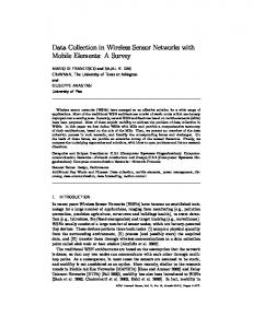
Figure 1: Optimal static scheduling strategy for a twocell symmetric network, R = 0.5 km. The cell capacity is then given by: c∗ = R ∗ R R dr −1 r dr . + 2 0 Cr,on r ∗ Cr,off Figure 2 compares the cell capacity obtained with and without interference avoidance. Now assume traffic is not uniformly distributed, but proportional to the distance to BS 1, so the total traffic load in cell 2 is three times that in cell 1. Besides the cell capacity obtained with and without interference avoidance, we are interested in the impact of load balancing where the cell radii R1 , R2 , with R1 + R2 = 2R, are set

Network capacity (bit/s/Hz)

10

With inter-cell scheduling Without inter-cell scheduling

8 6 4 2 0

0

0.5

1

1.5

2

2.5

3

Cell radius (km) 10 Network capacity (bit/s/Hz)

5.1 Radio environment We consider a continuous setting where the feasible rate of a user located at x is Cx,A when the set of active BS’s is A. We assume that the feasible rate depends on the signal-to-noise ratio (SNR) through the Shannon formula Cx,A = W log2 (1 + SNRx,A ), where W represents the bandwidth and SNRx,A is the SNR of a user located at x when the set of active BS’s is A. The Shannon formula provides a reasonable approximation of most real systems, up to a multiplicative constant. Let yn be the location of BS n. For any x in the cell of the reference BS, say BS 0, we get for isotropic radio propagation:

Both Inter-cell sched. only Load balancing only Nothing

8 6 4 2 0

0

0.5

1

1.5 2 Cell radius (km)

2.5

3

Figure 2: Capacity of a two-cell symmetric (left) or asymetric (right) network.

to equalize the cell loads: Z R1 Z R1 +R2 rdr rdr = . C C r,on r,on 0 R1 The corresponding cell capacity with and without interference avoidance can be derived from the results of §4.2. We observe in Figure 2 that load balancing increases the capacity of large cells where interference has a limited effect. On the other hand, load balancing is inefficient for small cells where interference is strong, and can even have a negative impact in this case. This is due to the fact that load balancing tends to maximize the use of the transmission resources, that is to use all BS’s at the same time, which in turn maximizes interference. This example highlights the fact that load balancing and interference avoidance are somewhat contradictory schemes. While load balancing tends to make all BS’s active to maximize the use of their transmission resources, interference avoidance aims at forcing some BS’s to be idle to limit the impact of interference on edge users. Thus, while load balancing is most efficient in sparse, noise-limited networks, interference avoidance is most efficient in dense, interference-limited networks. 5.3 Coordinating three BS’s Assume now that we wish to coordinate three BS’s. These BS’s are serving 3 facing sectors in an infinite tri-sectorized hexagonal network as depicted in Figure 3. User classes are indexed by (r, θ), r representing the distance to the BS and θ the angle to the center of the beam. A base of symmetric sets of BS’s is given by A1 = {1, 2, 3}, A2 = {1, 2}, A3 = {1}, with respective densities d1 = 1, d2 = 2/3, d3 = 1/3, and permutation

BS −1

BS 0

BS 1

R < 0.5 km 6

With Inter-cell Scheduling Without Inter-cell Scheduling

5 Cell capacity (bit/s/Hz)

σ(r, θ) = (r, −θ). For the sake of simplicity, we assume that all the BS’s except the three considered BS’s are always active. Figure 3 compares the cell capacity obtained with and without interference avoidance. The capacity gain may be as high as 33% for dense networks, a high value given the limited degree of coordination between the BS’s. This observation is especially relevant, since deployment scenarios are projected to evolve towards micro- and pico-cellular structures in areas where capacity matters the most.

4 3 2 1 0

R < 0.5 km 3.5

With inter-cell scheduling Without inter-cell scheduling

Cell capacity (bit/s/Hz)

3

0

0.5

1

1.5 2 Cell radius (km)

2.5

3

Figure 4: Optimal static scheduling strategy (left) and capacity (right) of a linear network.

2.5 2 1.5 1 0.5 0

0

0.5

1 1.5 2 Cell radius (km)

2.5

3

strategy uses two transmission profiles only: that where all BS’s are active and that where the closest interfering BS is turned off, corresponding to the star set 1. The optimal scheduling strategy is again roughly the same for sufficiently small cells and represented in Figure 6.

Figure 3: Optimal static scheduling strategy (left) and capacity (right) of a tri-sectorized hexagonal network.

Figure 7 gives the cell capacity with and without interference avoidance. The capacity gain may be as high as 25% for dense networks.

5.4 Linear networks Consider now an infinite linear network as depicted in Figure 4. Two successive BS’s are separated by a distance 2R. This is a symmetric network with classes indexed by r ∈ (−R, R). The sets A1j = {jk, k ∈ Z}, j ≥ 1, and A2j = {jk, jk + 1, k ∈ Z}, j ≥ 3, form a base of symmetric sets of active BS’s with respective densities d1j = 1/j, d2j = 2/j and permutation σ(r) = −r. It turns out that the optimal static scheduling strategy uses two transmission profiles only: that where all BS’s are active, corresponding to the set A11 , and that where the closest interfering BS is turned off, corresponding to the set A23 . A class r is served when all BS’s are ∗ on if and only if r < r ∗ , with r∗ such that Cr,A = 11 ∗ ∗ 2/3 × Cr,A23 . We observed that the ratio r /R is almost constant and approximately equal to 0.54 for sufficiently small cells, R < 0.5 km say. 5.5 Hexagonal networks Finally, we consider an infinite hexagonal network. This is a symmetric network with classes indexed by (r, θ) as in §5.3. If infinite, the symmetric set is either the whole network, a ‘stripe’ set or one of the three ‘star’ sets depicted in Figure 5, where the stripe set of highest density is also represented. The permutation defining the base of symmetric sets is σ(r, θ) = (r, θ + π/3). Again, it turns out that the optimal static scheduling

6 Conclusion We have evaluated the potential capacity gains from inter-cell scheduling in a dynamic setting, and specifically focused on interference avoidance in ‘TDMA networks’. Numerical experiments indicate that interference avoidance yields the largest gains in dense, interference-limited networks, ranging from 25 to 50%, depending on the network topology. This finding is particulary relevant, because deployment scenarios are anticipated to move towards micro- and pico-cellular networks in areas where traffic load is high and capacity is critical. In sparse, noise-limited networks, the gains from interference avoidance alone are far smaller, but load balancing does help increase capacity in case of heterogeneous loads. Thus, the relative efficacy of interference avoidance vs. load balancing critically depends on the network configuration. Another key observation is that, in all considered examples, the optimal capacity is attained by the use of two transmission profiles only: that where all BS are on, and that where only the first interfering BS is switched off. This suggests that a limited degree of coordination is sufficient in practice to achieve the expected capacity gains. The design of the corresponding distributed scheduling schemes opens research perspectives of considerable practical interest.

Star set 1

Star set 2

Cell capacity (bit/s/Hz)

2

With inter-cell scheduling Without inter-cell scheduling

1.6 1.2 0.8 0.4 0

0

0.5

1

1.5

2

2.5

3

Cell radius (km)

Figure 7: Capacity of a hexagonal network. Star set 3

Stripe set

Figure 5: Star and stripe sets of respective densities 6/7, 3/4, 2/3, 2/3 and the corresponding potential service zones.

[9] T. Bonald, S.C. Borst, A. Prouti`ere (2004). Inter-cell scheduling in wireless data networks. CWI report. [10] T. Bonald, S.C. Borst, N. Hegde, A. Prouti`ere (2004). Wireless data performance in multi-cell scenarios. In: Proc. ACM Sigmetrics / Performance 2004. [11] T. Bonald, M. Jonckheere, A. Prouti`ere (2004). Insensitive load balancing. In: Proc. ACM Sigmetrics / Performance 2004. [12] T. Bonald, A. Prouti`ere (2003). Wireless downlink data channels: User performance and cell dimensioning. In: Proc. ACM Mobicom 2003, 339–352.

All BSs on

Star set 1

R < 0.5 km

Figure 6: Optimal static scheduling strategy for a hexagonal network.

REFERENCES

[13] S.C. Borst (2003). User-level performance of channelaware scheduling algorithms in wireless data networks. In: Proc. Infocom 2003. [14] J.W. Cohen, O.J. Boxma (1983). Boundary Value Problems in Queueing System Analysis. (North-Holland, Amsterdam). [15] S. Das, H. Viswanathan, G. Rittenhouse (2003). Dynamic load balancing through coordinated scheduling in packet data systems. In: Proc. Infocom 2003.

[1] 3GPP (2002). Spatial Channel Model Text Description SCM 077. http://www.3gpp.org.

[16] J.M. Holtzman, S. Ramakrishna (1998). A scheme for throughput maximization in a dual-class CDMA system. IEEE J. Sel. Areas Commun. 40, 830–844.

[2] R. Agrawal, A. Bedekar, R.J. La, V. Subramanian (2001). Class and channel condition based weighted proportional fair scheduler. In: Teletraffic Engineering in the Internet Era, Proc. ITC-17, 553–565.

[17] A. Jalali, R. Padovani, R. Pankaj (2000). Data throughput of CDMA-HDR a high efficiency-high data rate personal communication wireless system. In: Proc. IEEE VTC 2000 Spring Conf., 1854–1858.

[3] D.M. Andrews, K. Kumaran, K. Ramanan, A.L. Stolyar, R. Vijayakumar, P.A. Whiting (2004). Scheduling in a queueing system with asynchronously varying service rates. Prob. Eng. Inf. Sc. 18, 191–217.

[18] X. Liu, E.K.P. Chong, N.B. Shroff (2003). A framework for opportunistic scheduling in wireless networks. Comp. Netw. 41, 451–474.

[4] M. Armony (1999). Queueing Networks with Interacting Service Resources. Ph.D. thesis, Stanford University. [5] N. Bambos, G. Michailidis (2004). Queueing and scheduling in random environments. Adv. Appl. Prob. 36, 293–317. [6] A. Bedekar, S.C. Borst, K. Ramanan, P.A. Whiting, E.M. Yeh (1999). Downlink scheduling in CDMA data networks. In: Proc. Globecom ’99, 2653–2657. [7] P. Bender, P. Black, M. Grob, R. Padovani, N. Sindhushayana, A. Viterbi (2000). CDMA/HDR: a bandwidth-efficient high-speed wireless data service for nomadic users. IEEE Commun. Mag. 38 (7), 70–77. [8] T. Bonald, S.C. Borst, A. Prouti`ere (2004). How mobility impacts the flow-level performance of wireless data systems. In: Proc. IEEE Infocom 2004.

[19] S. Ramakrishna (1998). Optimal Scheduling of CDMA Systems. Ph.D. thesis, WINLAB, Rutgers University. [20] A.L. Stolyar (2004). On the asymptotic optimality of the gradient scheduling algorithm for multi-user throughput allocation. Oper. Res., to appear. [21] L. Tassiulas, A. Ephremides (1992). Stability properties of constrained queueing systems and scheduling policies for maximum throughput in multi-hop radio networks. IEEE Trans. Aut. Control 37, 1936–1938. [22] V. Tsibonis, L. Georgiadis, L. Tassiulas (2003). Exploiting wireless channel state information for throughput maximization. In: Proc. Infocom 2003. [23] V. Viswanath, D.N.C. Tse, R. Laroia (2002). Opportunistic beamforming using dumb antennas. IEEE Trans. Inf. Theory 48, 1277–1294.