Hans-Peter Seidel. Max-Planck-Institut für Informatik. Saarbrücken, Germany. Abstract. This paper presents a rendering method for translucent objects, in which ...
Volume xx (200y), Number z, pp. 1–11
Interactive Rendering of Translucent Objects Hendrik P.A. Lensch
Michael Goesele
Marcus A. Magnor
Philippe Bekaert
Jochen Lang
Jan Kautz
Hans-Peter Seidel
Max-Planck-Institut für Informatik Saarbrücken, Germany
Abstract This paper presents a rendering method for translucent objects, in which view point and illumination can be modified at interactive rates. In a preprocessing step, the impulse response to incoming light impinging at each surface point is computed and stored in two different ways: The local effect on close-by surface points is modeled as a per-texel filter kernel that is applied to a texture map representing the incident illumination. The global response (i.e. light shining through the object) is stored as vertex-to-vertex throughput factors for the triangle mesh of the object. During rendering, the illumination map for the object is computed according to the current lighting situation and then filtered by the precomputed kernels. The illumination map is also used to derive the incident illumination on the vertices which is distributed via the vertex-to-vertex throughput factors to the other vertices. The final image is obtained by combining the local and global response. We demonstrate the performance of our method for several models. Categories and Subject Descriptors (according to ACM CCS): I.3.3 [Computer Graphics]: Picture/Image Generation Display Algorithms I.3.7 [Computer Graphics]: Three-Dimensional Graphics and Realism Color Color, Shading, Shadowing and Texture I.3.7 [Computer Graphics]: Three-Dimensional Graphics and Realism Color Radiosity
1. Introduction On the appropriate scale, the visual appearance of most natural as well as synthetic substances is profoundly affected by light entering the material and being scattered inside 9 . Examples of materials whose macroscopic appearance depends on the contribution from subsurface scattered light include biological tissue (skin, leaves, fruits), certain rocks and minerals (calcite, fluorite, silicates), and many other common substances (snow, wax, paper, certain plastics, rubber, lacquer). Depending on the scale of display, conventional, surface-based reflection functions may only unconvincingly mimic the natural visual impression of such materials (see Figure 1). Previous rendering algorithms handling subsurface scattering do not nearly allow interactive image synthesis (see Section 2 for an overview). However, light particles traveling through an optically dense medium undergo frequent scattering events causing severe blurring of incident illumination. The rendering method proposed in this paper takes advantage of this smoothing property of highly scattering submitted to COMPUTER GRAPHICS Forum (1/2003).
Figure 1: A back lit marble horse sculpture. Left: using a traditional surface based light reflection model. Right: taking into account subsurface scattering of light. Translucency effects are very clear in particular at the ears and the legs. The sculpture measures about 5cm head to tail. This paper presents a rendering method which convincingly reproduces translucency effects as shown in the right image, under dynamic viewing and illumination conditions and at interactive rates.
2
Lensch et al. / Interactive Rendering of Translucent Objects
media by factoring the light impulse response on the surface of a translucent object into a high frequency local part and a low frequency global part. We show that the impulse response can be precomputed efficiently, stored compactly and processed rapidly in order to allow interactive rendering of translucency effects on rigid objects at interactive rates under dynamic viewing and lighting conditions.
���
� � 1 � Ft η � ωi Rd xi � xo Ft η � ωo π
� α e � σtr dr zr 1 � σtr dr 4π dr3
xi � ωi ; xo � ωo �
�
Rd xi � xo �
Usually in global illumination, one assumes that a scattered light particle leaves a lit surface at the location of incidence itself. The relation between the intensity of light scattered at x into an outgoing direction ωo and the intensity of incident illumination at x received from a direction ωi is given by the BRDF (bi-directional reflectance distribution function) fr x � ωi � ωo � . However, local light scattering is only a valid assumption for a metal surface or for a smooth boundary between non-scattering media. In other cases, a light particle hitting a surface at a first location xi from direction ωi may emerge at a different surface location xo .
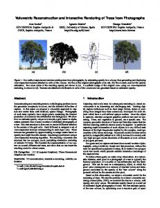
Non-local light scattering at a surface can however also be modeled explicitly, by means of the BSSRDF (bi-directional subsurface scattering reflectance distribution function) � xi � ωi ; xo � ωo � . BSSRDF models have been presented for single 6 and multiple 11 subsurface light scattering in homogeneous materials. These models can be used in a ray tracer, much in the same way as traditional BRDF models. The most prominent difference is that they require two surface locations rather than one. However, these BSSRDF models are much more complex than typical BRDF models (see for instance Figure 2), so that rendering times for common image resolutions still are in the order of seconds to minutes per frame.
dv
��
� �
A
Fdr
D
dr
The algorithm in this paper draws upon previous work in the areas of global illumination, real time local shading with complex BRDFs and database approaches for reflectance.
�
xr
xo � , with xr
�
xi � zr � Ni
1 � 3σt
��
σt
3σa σt
σs
σa � σs
;
α
σs � σt
reduced scattering coefficient (given)
relative refraction index (given)
σa
absorption coefficient (given)
η
Ft η � ω �
Ni
Fresnel transmittance factor
xi � xo
ωi � ωo
σtr dv
dv3
xv � xo � , with xv xi � zv � Ni 1 � Fdr 1 � Fdr 1 � 440 0 � 710 � η2 � η � 0 � 668 � 0 � 0636η
σtr
�
e�
zr � 4AD
zv
2. Previous Work
zv 1 � σtr dv
1 � σt
zr
This phenomenon can be simulated with a number of algorithms that have been proposed for global illumination in the presence of participating media, including finite element methods 21 � 1 � 23 , path tracing 6 , bi-directional path tracing 15 , and photon mapping 10 � 4 , or by a diffusion simulation 26 . Also, the propagation of electromagnetic radiation in scattering media is a well-studied topic outside of computer graphics in fields such as medical imaging, atmosphere and ocean research and neutron transport 9 � 25 . Methods for global illumination are often instances of methods used in these other fields. In optically dense media, such methods can be quite expensive, with typical image rendering times in the range from 10 minutes to several hours for static illumination and viewing parameters.
�
�
in- and out-scattering location (given)
in- and out-scattering direction (given) surface normal at xi (given)
1 0.1 0.01 0.001 0.0001 RED 1e−05 1e−06 1e−07
GREEN
0
2
4
6
8
10
12
14
16
BLUE 18
20
Figure 2: The BSSRDF model (from 11 ) used in this paper. Constants for some materials are also found in 11 . The graphs show the diffuse reflectance due to subsurface scattering Rd for a measured sample of marble with σs� =(2.19,2.62,3.00) ����� , σa =(0.0021,0.0041,0.0071) ����� and η=1.5. Rd r � indicates the radiosity at a distance r in a plane, due to unit incident power at the origin. Subsurface scattering is significant up to a distance of several millimeters in marble. The graphs also explain the strong color filtering effects observed at larger distances. � ��� RGB color triplet
Real-time rendering of objects with complex BRDFs has been done with a variety of techniques 2 � 8 � 13 � 12 . These techniques assume point light sources or distant illumination submitted to COMPUTER GRAPHICS Forum (1/2003).
Lensch et al. / Interactive Rendering of Translucent Objects
(environment maps) and usually do not allow spatial variation of the BRDF. None of these techniques can be applied to subsurface scattering for translucent objects, since the influence on incident light is not local anymore. Recent work on interactive global illumination of objects 24 , including self-shadowing and interreflections, can probably be extended to subsurface scattering. But this method assumes low-frequency distant illumination, whereas our method allows high-frequency localized illumination.
� or surface
16 5
Image-based techniques like light fields light field 18 � 28 represent the appearance of objects such that they can be interactively displayed for different views. The outgoing radiance is recorded and stored in a sort of database which then can be efficiently queried for assembling new views. Light fields can represent the outgoing radiance of an object which exhibits subsurface scattering under fixed illumination. Relighting of the object requires to additionally record the dependency on the incident illumination. Reflection fields 3 parameterize the incident illumination by its direction only. Although different illumination can be simulated by use of different environment maps, it is not possible for example to cast a shadow line onto the object. The directional dependency is not sufficient to represent local variation of the illumination on the object’s surface. Our approach for the representation of translucent objects takes the spatial variation of incident illumination into account while the directional dependency is not stored explicitly. This approach will be motivated in the following section. 3. Background and Motivation In order to compute the shade of a translucent object at a surface point xo , observed from a direction ωo , the following integral needs to be solved: L!
xo � ωo �#"%$
$
L'
S Ω & xi
� �
xi � ωi � � xi � ωi ; xo � ωo � dωi dxi (
S denotes the surface of the object and Ω ) xi � is the hemisphere of directions on the outside of the surface at xi . Note that the BSSRDF � , which represents the outgoing radiance at xo into direction ωo due to incident radiance at xi coming from direction ωi , is an eight-dimensional function, so that naive precomputation and storage approaches are not feasible in all practical cases. Previous subsurface scattering studies 6 � 11 however reveal * that: subsurface scattering can be accurately modeled as a sum
* of a single scattering term and a multiple scattering term;
single scattering accounts for at most a few percent of the outgoing radiance in materials with high scattering albedo, like marble, milk, skin, etc. . . — we will ignore * single scattering in this work; multiple scattering diffuses incident illumination: any relation between directions of incidence and exitance is lost. submitted to COMPUTER GRAPHICS Forum (1/2003).
3
As a result, subsurface scattering in highly scattering materials can be represented to an accuracy of a few percent by a four-dimensional diffuse subsurface reflectance function Rd xi � xo � , which relates scattered radiosity at a point xo with differential incident flux at xi : L!
xo � ωo �+" B xo �+" $ E xi �+",$
1 Ft η � ωo � B xo � π S
(1)
E xi � Rd xi � xo � dxi L'
Ω & xi
� �
(2)
xi � ωi � Ft η � ωi �.- Ni / ωi - dωi (3)
The Fresnel transmittance factors Ft indicate what fraction of the flux or radiosity is transmitted at a surface boundary. The Fresnel factor in Equation 3 indicates what fraction of incident light enters the translucent object. In (1), it models what fraction of light coming from underneath re-appears in the environment. The remainder re-enters the object, for instance due to total internal reflection if the object has a higher refraction index than its surrounding. A fast approximation of Fresnel factors has been proposed in 22 . The factor 1 0 π in (1) converts radiosity into exitant radiance. The diffuse subsurface scattering reflectance Rd in (2) plays a somewhat similar role as the radiosity integral kernel G x � y � in the radiosity integral Equation B x �1" G x � y �1"
Be x �32 ρ x �4$
S
G x � y � B y � dy
(4)
- Nx / ωxy -5- Ny / ωxy - vis x � y �( π6 x 7 y6 2
where B x � denotes the radiosity at x, Be x � the self-emitted radiosity, ρ x � the reflectivity, ωxy the direction of a line connecting x and y and vis x � y � is the visibility predicate. Factors like G x � y � in radiosity and Rd xi � xo � in our case, are usually called (differential) throughput factors. The main idea of this paper is to discretize Equation (2), much in the same way as the the radiosity integral equation (4) is discretized in Galerkin radiosity methods 7� 29 . The throughput factors that result from discretization of the radiosity equation are better known as form factors. Note however that form factors in radiosity encode purely geometric information about a scene to be rendered and that they do not directly allow to re-render a scene under dynamic lighting conditions. The subsurface scattering reflectance Rd xi � xo � encodes besides geometric information also the volumetric material properties anywhere in the object relevant for light transport from xi to xo : it is the Green’s function (impulseresponse, global reflectance distribution function 14 ) of the volumetric rendering equation inside the object. In radiosity, the Green’s function does in general not result in practical relighting algorithms due to its high storage cost. The primary goal of this paper is to demonstrate that explicit representation of the Green’s function however is practical for dynamic relighting of translucent objects. This is because
4
Lensch et al. / Interactive Rendering of Translucent Objects
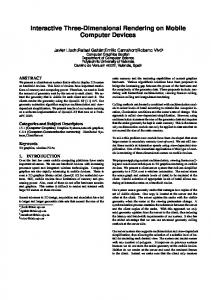
Figure 3: Work flow during rendering: first, incident illumination is computed and projected into the texture atlas. The resulting illumination map is processed in two ways. The global response (upper branch) is computed by projecting the illumination to the mesh vertices and multiplying the vertex irradiance vector with a vertex-to-vertex throughput factor matrix. The local response (lower branch) is computed by filtering the incident illumination map with spatially varying 7 8 7 texel-to-texel filter kernels. Finally the global and the local response are combined.
Rd is in general a much smoother function than the Green’s function for radiosity. In this paper, we will use the diffuse sub-surface scattering reflectance model from 11 (see Figure 2). This model has been derived for scattering at a planar boundary surface between homogeneous materials. It is in principle not valid for curved surfaces and neither for heterogeneous materials, although using it in such cases often yields plausible results. This paper however focuses on the feasibility of storing and using the Green’s function for interactive rendering of translucent materials. A proper treatment of curved surfaces and heterogeneous materials requires a more sophisticated preprocessing than shown here, and is the topic of future work. However, it does not affect the rendering algorithm itself proposed in this paper.
2. We project the irradiance E x � (Equation 3) onto the chosen basis: the coefficients Ei in E˜ x ��" ∑i Ei ψi x ��9 E x � , are found by calculating scalar products of E x � with dual ˜ i x� : basis functions ψ
$ E x � ψ˜ i x � dx
Ei "
(5)
S
The dual basis functions are the unique set of linear combinations of the primary basis functions ψ x � that fulfill the following orthonormality relations:
$ ψi x � ψ˜ j x � dx " δi j ( S
δi j denotes Kroneckers delta function (1 if i " j, 0 otherwise); 3. Equation 2 is transformed into a matrix-vector multiplication: Bj "
4. Outline
∑ Ei Fi j
(6)
i
Our method is based on a discrete version of the integral expression in Equation 2 at which we arrive with a Garlekin type approach. In this approach we employ two different sets of basis functions arriving at two different discretization. One set of basis functions are hat functions placed at object vertices in order to model subsurface scattering at large distances (smooth global part). The other set of basis functions are piecewise constant corresponding to the texels in a texture atlas (discussed below) in the immediate neighborhood of a point, in order to accurately model Rd at small scattering distances (detailed local part). Each of the two discretizations proceed as follows:
4. The radiosity B y � at surface position y is reconstructed as
1. We fix a set of spatial basis functions ψi x � . The basis functions we use are discussed below;
Two discrete representations of the same problem are of course redundant. We apply such a double representation to
with throughput factors Fi j "%$
$ ψi x � Rd x � y � ψ˜ j y � dydx
(7)
S S
B y �:9
∑ B jψ j j
y� (
(8)
Equation 1 shows how radiosity is converted into outgoing radiance for a particular direction.
submitted to COMPUTER GRAPHICS Forum (1/2003).
Lensch et al. / Interactive Rendering of Translucent Objects
5
ing simplification we try to obtain equilateral triangles of similar size.
Figure 4: Example of a texture atlas for the bird model. Inner triangles are drawn in green, border triangles are marked in red.
exploit the advantages of each, however appropriate blending will be necessary for correct results. The work flow for rendering an image is illustrated in Figure 3. Our method has to address the following sub-problems, which are discussed in detail below: * Preprocessing: generation of a texture atlas for the input model; computation of throughput factors from each texel to a 9 8 9 texel neighborhood (detailed local response); computation of weights for distributing the illumination in each texture atlas texel to the nearest triangle vertices as well as for reconstructing the illumination from the nearest triangle vertices and computation of vertex-to-vertex throughput factors (smooth global response); computation * of factors for blending the local and global response; At rendering time: computation of the irradiance in each texture atlas texel (incident illumination map); distribution of the irradiance in each texel to triangle mesh vertex irradiance and application of the precomputed vertex-tovertex throughput factors in order to obtain the scattered radiosity at each vertex (global response); convolution of the incident illumination map with the precomputed texture filter kernels (local response); blending of local and global responses using the precomputed blending factors. 5. Preprocessing The preprocessing phase of the proposed algorithm consists of two steps – the generation of a texture atlas for the input model and the calculation of the local and global light distribution for light hitting an object at a single point (Green’s functions). 5.1. Geometry Preprocessing All rendering results presented here are based on triangle models which are reduced to less then 20000 triangles. Dursubmitted to COMPUTER GRAPHICS Forum (1/2003).
To obtain a 2D parameterization of the object surface, we generate a texture atlas. The atlas is generated by first splitting the triangular mesh of the model into different partial meshes and orthographically projecting each partial mesh onto a suitable plane. The angle between the normals of the projected triangles and the plane normal are kept small to avoid distortion and ensure best sampling rate. Starting with a random triangle, we add an adjacent triangle to a partial mesh if the deviation of the triangle’s normal compared to the average normal of the partial mesh is below some threshold, e.g. 30 degrees. We also add to each partial mesh a border formed by adjacent triangles. The width of the border is required to be at least 3 texels to provide sufficient support for applying the 7 8 7 filter kernels to the core of the partial mesh. The border triangles may be distorted in order to fulfill this constraint. All projected partial textures are rotated to ensure that the area of their axis-aligned bounding box is minimal 27 � 20 . A generic packing algorithm generates a dense packing of the bounding boxes into a square texture of predefined size. The algorithm is able to scale the size of the bounding boxes using a global scaling factor in order to ensure dense packing. Figure 4 shows an example texture atlas for the bird model. 5.2. Global response Subsurface scattering at larger distances tends to be very smooth and amenable to representation by means of vertexto-vertex throughput factors using linear interpolation of vertex radiosities. Linear interpolation of vertex colors is well-known in graphics under the name of Gouraud interpolation. On a triangle mesh, it corresponds to representing a color function by its coefficients w.r.t. the following basis functions: ψg1 x �;" β1 x �
;
ψg2 x � v . The basis functions are � � 1 on the part S u � v � of the model surface projected in a single texture atlas texel u � v � and they are 0 everywhere else. There is one such basis function per non-empty texture atlas ˜ l u > v are piecewise contexel. The dual basis functions in ψ � � stant in the same way, except that they take a value 1 0 A u � v � instead of 1 on S u � v � . A u � v � is the area of S u � v � and is computed as a side result of texture atlas generation. By Equation 5, the irradiance coefficients E l u � v � correspond to the average irradiance on S u � v � . We will approximate them by the value at the center point in the texel. The texel-to-texel throughput factor (7) between texel u � v � and s � t � is approximated as K u > v s � t �?" � � A u � v � Rd xc u � v � � xc s � t �@� with Rd being evaluated at the surface points xc corresponding to the center of the texels. These texel-to-texel throughput factors can be viewed as non-constant irradiance texture filter kernels. Equation 6 then corresponds to a convolution of the irradiance texture. The convolved (blurred) texture shows the locally scattered radiosity Bl y � . 5.4. Blending Local and Global Response The global and the local response cannot be simply added to obtain the correct result. In the regions of direct illumination, both contributions will add up to approximately twice the correct result. However, the radiosity Bg calculated in
Figure 5: a) Ideal impulse response. b) Local response modeled by the filtering kernel (red) c) Linear interpolation of the global response resulting from distributing the irradiance and evaluating the form factor matrix F. d) Optimized global and local response: The diagonal of F0 is set to zero, the weights for Bdi (green dots) are optimized to interpolate the boundary of the filter kernel (blue dots), the blue area is subtracted from the filter kernel.
Section 5.2 will have the largest interpolation error near the point of light incidence while Bl (Section 5.3) returns the more accurate response for points close to direct illumination (see Figure 5). Bl is actually only available for those points. Our choice is to keep the texel accurate filter kernel for the local radiosity since it represents the best local response of our model. Thus, we somehow have to reduce the influence of the low-frequency part at small scattering distances and must ensure smooth blending between the local and global response where the influence of the local response ends. The global radiosity Bg due to direct illumination corresponds to the diagonal of the form factor matrix F. The diagonal entries are set to zero yielding F0 . To obtain smooth blending we introduce a new radiosity vector Bdi which is directly derived from the illumination map in a way described below. Using this new radiosity vector, the combined radiosity response will be obtained as Bl x �32 Bd x �32 Bg0 x �
B x �A" Bgj 0
"
∑ Eig Fi0j
(9)
i
For each texel u � v � of the illumination map, we have to determine its optimal contribution wi u � v � to the direct radiosity Bdi of the three vertices vi of the enclosing triangle. Our approach is to minimize the difference between the global radiosity and the correct radiosity for each texel s � t � on the boundary Γ of its filter kernel K u > v s � t � . The correct � � radiosity at Γ is found by calculating a larger filter kernel 9B 9 K u > v s � t � . Notice that the influence of the 7 8 7 kernel on � � Γ of the 9 8 9 kernel is exactly zero. Stated mathematically, submitted to COMPUTER GRAPHICS Forum (1/2003).
Lensch et al. / Interactive Rendering of Translucent Objects
the problem is to find wν u � v � so that ∑ s> t � D� C
Γ
frame buffer and stored. In Figure 3a) and b) the illumination on the object and the corresponding illumination map derived using the texture atlas are shown.
9B 9 g0 E K� u > v � s � t � E u � v � 7 B xc s � t �F�
7 E u � v� /
3
∑ ψgν
νG 1
x u � v �@� wν u � v �IH
7
2
is minimal. xc s � t � is the surface point corresponding to the g g center of texel s � t � and Bg0 x �;" ∑ν ψν x � Bν0 . The sum is g over the vertices ν of the triangle containing x, and Bν0 is given in Equation 9. After correcting the global response, we also have to change the filter kernels. The interpolated values of the global response have to be subtracted from each kernel, corresponding to the blue area in Figure 5. This optimization has to be done for every texel. It is performed as a preprocessing step and takes just a few minutes. The irradiance at each texel is now distributed to two differg ˜ g and to ent vectors: to Ei using the dual basis functions ψ d the Bi using the weights w described in this section. 6. Rendering After preprocessing, the rendering is straightforward. In order to render a translucent object interactively, we first compute an illumination map and then split the computation into two branches. The first one derives the irradiance at each vertex from the illumination map and computes the smooth global response. The second branch evaluates the local response by filtering the illumination map. Both branches can be executed in parallel on a dual processor machine. Finally, the global and the local response are combined.
Once the irradiance at each texel u � v � is computed, we can integrate it to obtain the irradiance for each vertex. In order to distribute the texel irradiance correctly to vertex irradiance, we follow Equation 5. The vertex irradiance Eig is given as g
Ei "
∑ ψ˜ i
g
�
u> v
�
u � v� E u � v� A u � v� �
(10)
the sum over all texels in the illumination map times the value at the current texel of the dual basis function corresponding to the vertex, times the area A u � v � of the model surface S u � v � covered in the texel. As a result, the illumination at each texel is distributed to exactly three different ˜ gi u � v � A u � v � are precomputed into vertices. The weights ψ an image of the same resolution as the texture atlas. The same distribution mechanism is also applied to obtain the second radiosity vector Bdi (Section 5.4). This time, the weights wi u � v � are used instead of the dual basis function. Distributing the illumination map to two vectors instead of just one does not significantly influence rendering performance. 6.2. Low Frequency Reconstruction Given the irradiance at the vertices, the low frequency or global response is calculated with the throughput factors of Section 5.2. The resulting radiosity Bgi at the vertices based on the transfer functions matrix F is then found by g
Bj "
∑ Ei Fi j ( g
(11)
i
6.1. Computing the Illumination For an illuminated object, we need to convert its illumination from object space into texture space since the precomputed filter works in texture space. Furthermore, we have to integrate over the illumination map in order to compute the irradiance at the vertices. For the conversion to texture space we use the parameterization of the object given by the texture atlas. The illumination map can be created easily by rendering the object by not using its 3D vertex positions but its 2D texture coordinates from the texture atlas. This flattens the object according to the atlas and the result is a texture containing the illumination. Some care has to be taken that the lighting is computed correctly even though the geometry is projected into 2D. We do this by computing the lighting in a vertex shader 17 using the original 3D vertex position and normal. Furthermore, we include a Fresnel term in the lighting calculations for which we use Schlick’s approximation 22 , which can be computed in the vertex shader as well. The rendered illumination map is then read back from the submitted to COMPUTER GRAPHICS Forum (1/2003).
As previously discussed, the radiosity at a particular point x on a triangle is interpolated using the barycentric basis g ψν x � with respect to the vertices of the triangle. Bg x �#"
3
∑ ψν
νG 1
g
g
x � Bν
(12)
Depending on the size of the model and the scattering parameters, the entries in the matrix may drop to very small values. In these cases a full N 8 N matrix times vector multiplication may be more costly than ignoring form factors below 10 J 5 using just a sparse matrix. In our experiments the overhead of representing a sparse matrix paid off if 40 percent of the form factors could be ignored. If desired, surface appearance detail can be added by means of a surface texture Tρ which modulates the radiosity. Tρ represents the overall reflectance at each texel. Since the form factor matrix F already computes the radiosity at the vertices correctly, we have to ensure that those values are not changed by the texture. Therefore we divide the vertex
8
Lensch et al. / Interactive Rendering of Translucent Objects
radiosity by its corresponding texture value prior to multiplication with the texture: BTi " Bgi 0 Tρ vi �
(13)
The complete low-frequency response is then given by Bg x �