Proceedings of the Fourth IASTED International Conference SIGNAL AND IMAGE PROCESSING August 12-14, 2002, Kaua’i, Hawaii, USA
Interactive Shape Preserving Filtering and Visualization of Volumetric Data Arnold Meijster Centre for High Performance Computing & Visualization University of Groningen P.O. Box 800, 9700 AV, Groningen, The Netherlands email:
[email protected] ABSTRACT This paper presents a method for combined interactive filtering and visualization of volumetric data. The user can set the filter parameters of a shape preserving class of morphological filters, called connected filters, efficiently. The filters work by computing some attribute describing the shape or size for each connected component, and then deciding which to keep based on some threshold. We use a method in which the computation of attributes and connected component analysis is separated from the decision stage of the filtering process. After performing the first stage as initialization, we can perform the (much faster) decision stage many times with different threshold values, allowing interactive filtering and visualization of the results. The results indicate that filtering can be performed at about 5 frames per second on a 2563 data set using a Pentium 4 at 1.9 GHz.
Figure 1. Decomposition of binary image of nuts and bolts of different sizes into different shape classes: (left) original image; (middle) filter with criterion “number of holes > 0”; (right) difference between (left) and (middle).
for each connected component, and then deciding which to keep based on, e.g., some threshold or window on these parameter values. An example is shown in Fig. 1, in which the nuts are separated from the bolts based on the number of holes. In grey scale, attribute filters can be implemented simplistically by thresholding the image at each grey level, applying a binary filter to each, and recombining them. Faster algorithms have been developed [1], but in the case of volumetric data, filtering is still too slow to be interactive in many cases. For example, filtering of a 2563 data set for vessel enhancement may take 12 s even on a Pentium 4 at 1.9GHz with 800 MHz RDRAM. This is a serious drawback when optimal threshold settings are being determined for the filtering process. In this paper, we use a method first proposed by Salembier et al. [2], in which the computation of attributes and connected component analysis (stage 1) is separated from the decision of the filtering process (stage 2). After performing the first stage as initialization, we can then perform the (much faster) decision stage many times with different threshold values, allowing interactive filtering and visualization of the results.
KEY WORDS shape filters, volume visualization, interactive filtering
1
Introduction
In this paper, we present a method for combined filtering and visualization of volumetric data in such a way that the user can set the filter parameters efficiently, allowing filtering at interactive rates. We use a shape preserving class of morphological filter called connected filter. Connected filters have received much attention in recent years, in algorithm development [1, 2], and applications [3, 4]. Connected filters are shape preserving, because they never introduce new edges in images. A subclass of these are attribute filters, the first of which were area openings and closings, which remove image detail smaller than a particular area [5]. These in turn were extended to attribute openings which accept or reject image details based on any of a wide range of size parameters [6]. They also put forward the idea of attribute thinnings, which allow image filtering based on shape, rather than size criteria. This idea has been formalized to so called shape filters [7], which have been applied to the problem of vessel enhancement in angiographic volume data sets [4]. In the binary case, attribute filters work by computing some parameter (or attribute) describing the shape or size 359-165
Michel A. Westenberg and Michael H. F. Wilkinson Institute of Mathematics and Computing Science University of Groningen P.O. Box 800, 9700 AV, Groningen, The Netherlands email: {michel, michael}@cs.rug.nl
2
Filtering using Max-Trees
An efficient implementation of attribute filters relies on computing both the hierarchy of connected components in the data set, and some attribute for each component to 640
use as a filter criterion. A Max-Tree representation of the dataset was introduced by Salembier et al. [2] as a more versatile structure to separate the filtering process from the computation of connected components and attributes. The building of this tree structure is called the construction phase, while its use for filtering is called the filtering phase. In this section we will briefly discuss this data representation, and how it can be used to perform filtering. Let M ⊆ Rn be some image domain (n = 2 for images, n = 3 for volumes), and f : M → R the grey scale image (volume) under study. Implicitly we assume the existence of some neighborhood graph (i.e. a grid) on M. A Max-Tree is a tree where the nodes represent sets of flat zones or connected components of f . A set F ⊂ M is called a flat zone or connected component if for all p, q ∈ F there exists a path from p to q along which the function value is constant, and the set M is maximal in size. The threshold set Xh (f ) of image f is the set of points that remain after thresholding at level h, i.e. Xh (f ) = {x ∈ M|f (x) ≥ h}.
P30 P20 P21 P10 P00
C30 ? C20 C21 @ R 0 @ C1 ? C00
20 8 6 50 70
Figure 2. The peak components of a grey level image X (left), the corresponding attributes (middle) and the MaxTree (right)
P10 P00
Min P30 P10 P00
Direct
(1)
P30 P20 P10 P00
Max P20 P10 P00
Subtractive
Figure 3. Result after filtering the signal in Fig. 2 with four different decision rules, using λ = 10 as the attribute threshold
A peak component at a grey level h is a connected component of the threshold set Xh (f ). The number of these peak components is finite and can thus be enumerated. We introduce the notation Phk to denote the kth peak component at level h. Max-Tree nodes are connected components, and therefore there exists a unique mapping from Max-Tree nodes to peak components. We use the notation Chk to denote the node that consists of the subset of Phk with grey level h. The root node represents the set of pixels belonging to the background, that is the set of pixels with the lowest intensity in the image. The Max-Tree is a rooted tree: each node has a pointer to its parent, i.e. the nodes corresponding to the components with the highest intensity are the leaves (see Fig. 2). Hence the name Max-Tree: the leaves correspond to the regional maxima. This means that the Max-Tree can be used for filters that process peak components, i.e. starting from the regional maxima. Conversely, a tree in which the leaves correspond to the minima is called a Min-Tree and can be used for filters that process valley components, i.e. starting from the regional minima. During the construction phase, the Max-Tree is built from the flat zones of the image. After this, the tree is processed during the filtering phase. This filtering removes flat zones based on some property. These properties are defined by an attribute value T (Phk ) of a node Chk , from an ordered universe (typically R or Z) on which an order ≤ exists. Given a threshold value λ from this universe, the algorithm decides whether to preserve, or remove a node. Two classes of strategies exist:
• non-pruning strategies, in which the parent pointers of children of Chk are updated to point at the oldest “surviving” ancestor of Chk . Salembier describes four different rules for the algorithm to filter the tree: the Min, the Max, the Viterbi, and the Direct decision. The first three are pruning strategies. In addition, Wilkinson and Urbach [7] introduced another non-pruning strategy, called the Subtractive decision. The decisions of these rules are as follows: Min A node Chk is removed if T (Phk ) < λ or if one of its ancestors is removed. Max A node Chk is removed if T (Phk ) < λ and all of its descendant nodes are removed as well. Viterbi The removal and preservation of nodes is considered as an optimization problem. For each leaf node the path with the lowest cost to the root node is taken, where a cost is assigned to each transition. In this paper we do not consider this rule. For details see [2]. Direct A node Chk is removed if T (Phk ) < λ; its pixels are lowered in grey level to the highest ancestor which meets the criterion, its descendants are unaffected. Subtractive As above, but the descendants are lowered by the same amount as Chk itself.
• pruning strategies, which remove all descendants of Chk , if Chk is removed
Figure 2 shows the peak components of a 1-D discrete signal, their attribute values, and the corresponding 641
Max-Tree. The results of applying the Min, Max, Direct and Subtractive methods on this image with λ = 10 are shown in Fig. 3. Which of these rules is the most appropriate depends mainly on the application. Consider an image with just three nested peak components P31 ⊂ P21 ⊂ P11 at intensity levels 3, 2, and 1, respectively. Furthermore let T (P31 ) ≥ λ, T (P21 ) < λ, and T (P11 ) ≥ λ. No pruning strategy can simultaneously retain P31 and P11 , while removing P21 . Using the direct rule, the difference f − φTλ (f ), where φTλ (f ) is the filtered
Table 1. CPU times in seconds for non-interactive (building) and interactive (decision) phases of the Max-Tree algorithm for 3-D angiograms.
f − φTλ (f )
size
greylevels
building
decision
vessels
3
256
256
12.10
0.218
angio
2
1324
8.30
0.746
256 × 124
function using criterion T and threshold λ, will consist of a zero background with one or more connected regions at intensity level 1, consisting of those pixels of P21 which have intensity level 2, i.e. the members of C21 (which need not be connected). In general, a peak component of this image may satisfy the criterion. In the subtractive case, the difference image consists of only those peak components which do not satisfy the criterion. An example of these properties is shown in Fig. 4. The attribute used is I/A2 which is the moment of inertia divided by the square of the area. For a given object, the moment of inertia is minimal for a circle, and increases rapidly as the object becomes more elongated. In the case of the subtractive rule, the filtered image φTλ (f ) contains only elongated structures, and f − φTλ (f ) contains only compact structures.
Original image f
φTλ (f )
volume
φTλ (f − φTλ (f ))
Min
Max
3
Application to visualization
Salembier et al. [2] noted that the building phase of a MaxTree filter algorithm is by far the most costly. Therefore, given the fact that the Max-Tree algorithm is one of the fastest connected filter algorithms available, we assumed that the decision rule stage alone should work an order of magnitude faster than even the fastest method available [1]. For interactive filtering purposes, this would allow us to build the Max-Tree once, and use it repeatedly for filtering the image with different threshold levels. The speed gain was determined by comparing the time necessary to build the Max-Tree to the decision phase on different volume data sets. The results are shown in Table 1. The results indicate that, given fast rendering hardware, almost 5 frames per second can be reached on the 2563 data set on a Pentium 4 at 1.9 GHz, with 512 MB RDRAM. The smaller data set with larger number of grey levels gave slower timings, probably due to cache trashing. Figure 5 shows an example of an interactively filtered magnetic resonance angiogram volume data set, visualized by maximum intensity projection. The shape filter attribute used was I/V 5/3 , with I the moment of inertia and V the volume. This attribute is a purely shape dependent number, i.e. it is scaling invariant, which has a minimum value for a sphere and increases rapidly with elongation (see [4] for more details). The images show that by increasing the threshold parameter λ, more and more structures that are
Dir.
Sub.
Figure 4. Grey-scale decomposition of image using I/A2 > λ thinning with λ = 1.1 using two pruning (max and min) and two non-pruning filtering strategies. From left to right: filtered image φTλ (f ), difference image f − φTλ (f ) and filtered difference image φTλ (f − φTλ (f )) are shown for all four methods (the latter two columns have been contrast enhanced for clarity). The min filter removes the small bars within the larger circles from the image, whereas the max pruning strategy leaves the large circles in the filtered image. Of the non-pruning rules, the direct method has the problem that the difference image contains non-compact details, as can be seen by re-filtering with φTλ (third column)
642
not elongated disappear: for low threshold settings, only background noise is affected, and for a high threshold, only thin and very long structures remain. The user was supplied with a simple GUI containing a slider to set the threshold value λ. Since the filtering stage takes less than a second on datasets of this size, the user can interactively choose a threshold and view the result. For the particular example shown in Fig. 5, such interactive filtering can be of great assistance to a radiologist when dealing with noisy angiographic volume data.
4
[7] E. R. Urbach and M. H. F. Wilkinson. Shape-only granulometries and grey-scale shape filters. In Proceedings of the ISMM2002, in press.
Conclusion
In this paper, we have proposed a method for interactive filtering of volume data sets based on a class of shape preserving filters. We have briefly introduced such filters and how they can be implemented efficiently using Max-Trees. The Max-Tree approach splits the filtering task in two stages. The first stage is a construction of a tree, while the second stage performs actual filtering using this tree. Building the tree takes several seconds for small volumes, and up to 40 seconds for large volumes (i.e. 5123 ). However, after the construction of the tree, we have shown that a volume can be filtered in fractions of a second, allowing interactive filtering and visualization, even on standard commodity hardware like PCs.
References [1] A. Meijster and M. H. F. Wilkinson. A comparison of algorithms for connected set openings and closings. IEEE Trans. Patt. Anal. Mach. Intell., 24(4), 2002. in press. [2] P. Salembier, A. Oliveras, and L. Garrido. Antiextensive connected operators for image and sequence processing. IEEE Transactions on Image Processing, 7:555–570, 1998. [3] A. Sofou, C. Tzafestas, and P. Maragos. Segmentation of soilsection images using connected operators. In Int. Conf. Image Proc. 2001, pages 1087–1090, 2001. [4] M. H. F. Wilkinson and M. A. Westenberg. Shape preserving filament enhancement filtering. In W. J. Niessen and M. A. Viergever, editors, Medical Image Computing and Computer-Assisted Intervention, volume 2208 of Lecture Notes in Computer Science, pages 770–777, 2001.
Figure 5. Magnetic resonance angiogram volume data set (size 2563 ) filtered interactively with an attribute thinning as shape filter. The attribute used was I/V 5/3 , with I the moment of inertia, and V the volume of a peak component; the top left-hand image is the original, in the others the attribute threshold was 0.5, 1.0, 1.5, 2.0, 2.5, 3.0 and 4.0, respectively. This attribute is a shape dependent number that expresses elongation. Visualization was done by maximum intensity projection.
[5] F. Cheng and A. N. Venetsanopoulos. An adaptive morphological filter for image processing. IEEE Trans. Image Proc., 1:533–539, 1992. [6] E. J. Breen and R. Jones. Attribute openings, thinnings and granulometries. Computer Vision and Image Understanding, 64(3):377–389, 1996. 643