Evans, Lamont-Doherty Earth Observatory, greatly ... Dan Cayan and Larry Riddle at Scripps Institution .... A. Leetmaa, R. Reynolds, R. Jenne, and D. Joseph,.
Citation: Dettinger, M.D., Battisti, D.S., Garreaud, R.D., McCabe, G.J., and Bitz, C.M., 2001, Interhemispheric effects of interannual and decadal ENSO-like appear asina chapter in climate variations on theToAmericas, V. Markgraf (ed.), Interhemispheric Present and climate Past Interhemispheric linkages: Present Climate and PastLinkages Climates in in the the Americas Americas and Their their Societal Societal Effects Effects: Academic Press, 1-16. (V. Markgraf, ed., Academic Pess)
----------------------------------
INTERHEMISPHERIC EFFECTS OF INTERANNUAL AND DECADAL ENSO-LIKE CLIMATE VARIATIONS ON THE AMERICAS Michael D. Dettinger1, David S. Battisti2, McCabe, G.J.3, Cecilia M. Bitz4, and Rene D. Garreaud2 1
U.S. Geological Survey, Scripps Institution of Oceanography, 9500 Gilman Drive, La Jolla, CA 92093-0224 USA 2 Department of Atmospheric Sciences, University of Washington, Seattle, WA 98195-1640 USA 3 U.S. Geological Survey, Lakewood, Colorado USA 4 Quaternary Research Center, University of Washington, Seattle, Washington USA
Abstract Interannual El Niño/Southern Oscillation (ENSO) and decadal ENSO-like climate variations of the Pacific Ocean basin are important contributors to the year-to-year (and longer) variations of the climate of North and South America. Analysis of historical observations of global sea-surface temperatures, global 500 mb pressure surfaces, and western hemisphere hydroclimatic variations that are linearly associated with the ENSO-like climate variations yields striking cross-equatorial symmetries as well as qualitative similarities between the climatic expressions of the interannual and decadal processes. These similarities are impressive because, at present, the mechanisms that are believed to drive the two time scales of ENSO-like variability include several candidates that are quite dissimilar in terms of physical processes and locations. Despite potentially different source mechanisms, both interannual and decadal ENSO-like climate variations yield wetter subtropics (when the ENSO-like indices are in positive, El Niño-like phases) and drier midlatitudes and tropics (overall) over the Americas, in response to equatorward shifts in westerly winds and storm tracks in both hemispheres. The similarities of their continental-surface climate expressions may impede separation of the two ENSO-like processes in paleoclimatic reconstructions.
Resumen Variaciones asociadas con El Niño/Oscilación Sur (ENSO) a escala de tiempo de caracter interanual y decadal en el Océano Pacífico, resultan contribudores importantes del clima de Norte y Sur America. Analisis de los registros historicos de la temperatura de superficie del mar (SSTs), del campo global de nivel de la superficie a 500 mb, y de variaciones hidroclimáticas en el Hemisferio Occidental asociadas en forma lineal con variaciones de origen ENSO, exhiben simetrias marcadas en ambos hemisferios en la mayoria de sus expresiones de variabilidad climatica, en ambas escalas—interanual y decadal. Estas similaridades son notables, porque, al presente, los mecanismos que se creen responsables por las variaciones climaticas en estas dos escalas de variación temporal, vinculadas con fluctuaciones generadas por el fenomeno ENSO, incluyen varios candidatos, los cuales son asociados con distintos procesos físicos y zonas geográficas de acción. No obstante estos mecanismos potentialmente distintos, variaciones climaticas de escala interanual y decadal resultan en el desarrollo de condiciones mas lluviosas que lo normal en las regiones subtropicales (durante la fase calida del ENSO), y condiciones mas seca que lo normal en las latitudes medias y en los tropicos en general sobre el continente Americano. Esto ocurre en repuesta a los cambios de vientos de superficie en la zona ecuadorial de Pacifico, y cambios de las trajectorias de tormentas en ambos hemisferios. La similaridad de las expresiones climaticas en superficies en ambos hemisferios y escalas temporales, si acaso hará mas dificil la separación de las señales de indole paleoclimaticas de estas de variación del sistema ENSO. 1
Introduction A climatologist who specializes in modern climate variations was immediately struck, upon attending a workshop of the PoleEquator-Pole (PEP 1) Paleoclimate of the Americas Program, by the need to reconcile the various past climate reconstructions with climatic processes and conditions that we can recognize from instrumental climate variations. Some past-climate variations are recognizable; many are not. Indeed, on interannual and decadal timescales, the number of “typical” patterns of historical climate variation is limited. In the present climate, three climatic phenomena dominate climate variations in the Americas on interannual to decadal timescales. Best known is the El Niño/Southern Oscillation (ENSO) phenomenon, which dominates global climate variations on interannual timescales ranging (mostly) from 3 to 6 years; many climate studies have described this quasi-regular phenomenon of tropical air–sea interactions centered in the equatorial Pacific and its teleconnections to many parts of the globe (see reviews in Diaz and Markgraf 1992; Allan et al. 1996; Wallace et al. 1997). Less well characterized are decadal (10- to 50-year timescales) climate processes centered in the Pacific and in the Atlantic Ocean basins. On timescales longer than interannual, the dominant climate phenomenon in the Pacific Ocean and overlying atmosphere has an ENSO-like spatial distribution (Zhang et al. 1997, hereafter ZWB) of surface temperatures and atmospheric circulations and, as will be shown here, interhemispheric climate effects on the Americas. The physical processes responsible for this decadal ENSO-like variability remain uncertain but are tied to well-documented pan-Pacific changes in the atmosphere and ocean in the 1950s and mid1970s (Ebbesmeyer et al. 1991). Finally, decadal variability in the climate of the Atlantic basin also has a basin-wide signature
(Deser and Blackmon 1993; Hurrell 1995; Enfield and Mestas-Nuñez, 2000, this volume), but is somewhat distant from the cordillera of the Americas and thus will not be addressed here. In this chapter, modern interannual and decadal climate variations of the Pacific basin will be outlined and their interhemispheric climatic effects on the Pacific Ocean and the Americas will be compared. Several indices may be used to describe the historical variations of the ENSO and decadal ENSOlike phenomena, but often it is difficult to be sure that the two phenomena have been separated so that none of the climatic effects are attributed twice. Thus, a new set of uncorrelated indices for the two processes will be developed and used, alongside a pair of indices that have been used in the literature, to characterize oceanic, atmospheric, and landsurface climate variations associated with the ENSO-like phenomena. The construction of indices, and datasets that will be compared to those indices, will be described in the next section of this chapter. In subsequent sections, oceanic, atmospheric, and continental conditions that are linearly related to the interannual and decadal phenomena will be delineated by simple correlation and regression analyses. In the final two sections, the results will be discussed and conclusions summarized. Data and definitions Interannual and decadal climate variations in the Pacific Ocean basin can be traced through any of literally dozens of physical and biological indices (e.g., Ebbesmeyer et al. 1991). In this chapter, two sets of indices based on sea-surface temperature (SST) patterns of global scale will be used to depict the North Pacific climate and its effects on the Americas. Two indices developed by ZWB—the Cool Tongue (CT) index and the Global Residual (GR) index—will be discussed for the most
2
part but, for completeness, a second pair of indices based on a linear combination of some more commonly available time series— Southern Oscillation Index (SOI), the CT index, and the Pacific (inter)Decadal Oscillation (PDO) index—also will be considered. The origins and significance of these various indices are discussed below. Global SSTs were analyzed by ZWB using linear regressions and principal component (PC) analyses in order to separate interannual ENSO-related SST variations from other interannual and decadal variations and to describe those other SST variations.
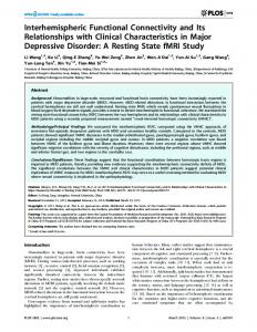
Interannual ENSO-related SST variations were characterized by the CT index, which is the average of SST anomalies from 6°N to 6°S, 180° to 90°W, an index previously used by Deser and Wallace (1990). This region is the locus of cool SSTs in the eastern equatorial Pacific, where the El Niño process has its clearest surface expression. Monthly mean SST anomalies on a 5° x 5° grid, from an updated version of the global United Kingdom Meteorological Office Historical Sea Surface Temperature Dataset (HSSTD; Folland and Parker 1990, 1995), were used to form this series (Fig. 1a), and then the CT series was
(a) Interannual, tropical indices
Dimensionless
4
CT INDEX TROPICAL PC INDEX
2 0 −2 −4 1910
1930
1950
1970
1990
(b) Decadal, extratropical indices
Dimensionless
4 GR INDEX N. PACIFIC PC INDEX
2 0 −2 −4 1910
1930
1950
1970
1990
Y Figure 1. (a) Unfiltered Cool-Tongue (CT) index and rotated “tropical” PC index, of dominantly interannual El Niño-Southern Oscillation (ENSO) variability in the tropical Pacific, and (b) Global Residual (GR) index and rotated “North Pacific” PC index, of dominantly decadal ENSO-like variability in the Pacific Ocean basin. The indices are described in the text. CT and GR indices are identical to those of Zhang et al. (1997).
3
high-pass filtered to remove variations with periods longer than 6 years, forming a strictly interannual series called CT*. The entire SST dataset then was regressed against the CT* time series, and the best linear fits at each grid point were subtracted from the grid-point SSTs to arrive at time series of residuals. By construction, these residuals are uncorrelated with the CT* series. A PC analysis of these residual series yielded a leading mode of “nonENSO” SST variation that was, surprisingly, very ENSO-like in its spatial patterns. This leading mode is called the GR index by ZWB and represents the decadal ENSO-like variations of the global and, especially, the Pacific SSTs (Fig. 1b). Although CT* and GR
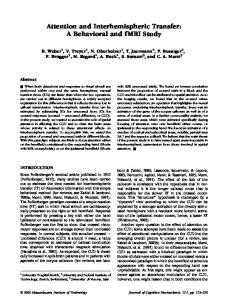
are not correlated, CT and GR are (r = -0.55). In this chapter, the interannual and decadal climate variations in the Pacific basin will be characterized in terms of these same CT and GR series; CT, rather than CT*, is used because it is more similar to such commonly used ENSO indices as the unfiltered SST indices along the equatorial Pacific in so-called Niño-3 and Niño-4 regions (e.g., Allan et al. 1996) than is the band-pass filtered CT*. The differing timescales of the CT and GR series can be demonstrated by spectral analysis. Shown in Figure 2 are multitaper power spectra (Percival and Walden 1993; Lees and Park 1995) of the two series. The CT spectrum (solid curve) indicates variance
Multitaper power spectra of CT and GR indices 1000 PC indices
Power
1000 100
100
10 0.0
0.4
Power
0.2
10
CT GR 1 0.0
0.1
0.2
0.3
0.4
Frequency, in cycles/year Figure 2. Multitaper power spectra of the Cool Tongue (CT) and Global Residual (GR) climate indices. The inset is a plot of the corresponding power spectra of rotated PC series: “tropical” PCs (solid curve) and “North Pacific” PCs (dashed curve). In the CT and GR spectra, at lowest frequencies, powers greater than about 80 to 200 exceed 95% confidence levels—not shown here—in comparisons to red noise (Mann and Lees 1996); at highest frequencies, power greater than about 30 reaches 95% confidence levels.
4
spanning a broad range of frequencies centered near 0.2 cycles/yr, corresponding to a period of 5 years. In contrast, GR has a spectrum that increases rather steadily from high frequencies to low, with a local maximum near 0.16 cycles/ yr. Thus GR is dominated by low-frequency variations with timescales between about 6 years and several decades; CT is dominated by interannual variations in the 3- to 7-year range. Recall that the CT series used here has not been temporally filtered; therefore, the interannual dominance of CT shown reflects the true mix of frequencies in the tropical Pacific ENSO variations. The GR index is derived as a residual from an interannually filtered CT* series (and its reflection in global SSTs) and thus, as a measurement of North Pacific climate variation, is biased by design toward the more decadal parts of Pacific climate variability. Alternative approaches and indices for characterizing the interannual and decadal modes of Pacific climate variation have been developed in the literature. Enfield and Mestas-Nunez (2000, this volume) used complex empirical-orthogonal function (EOF) analyses of global SSTs to arrive at similar modes. Mantua et al. (1997) used the CT index and a PDO index to describe essentially the same variability. The PDO index is defined, by Mantua et al. (1997), as the first PC of monthly SSTs, from the HSSTD, poleward of 20°N in the Pacific basin, initially calculated from anomalies for the period 1900-93. This index has a strong decadal character much like the GR index (and is correlated with GR at r = +0.74) but has not had any ENSO variability explicitly removed; indeed, its correlation with the CT series is r = +0.38. The PDO was intended to reflect the decadal variability of the North Pacific in a simple index but has a substantial expression throughout the tropical and South Pacific (see Fig. 3d here or Fig. 2a of Mantua et al. 1997). Tropical ENSO variability historically— e.g., Troup (1965) and most more recent
references—has been indexed by the SOI and SST anomalies in selected equatorial regions. The SOI is usually defined as the difference between standardized monthly departures of sea-level pressure (SLP) from their normal seasonal cycles at Tahiti and Darwin, Australia. When SLPs are low in the eastern tropical Pacific near Tahiti and high in the western tropical Pacific near Darwin (when SOI is negative), the tropical easterly winds become weak and the resulting slackening of equatorial upwelling of cool deep water in the eastern equatorial Pacific, together with a relaxation of warm waters from the western Pacific into the usually cool eastern Pacific, leads to warmer than normal SSTs in the eastern equatorial Pacific. These episodes of warm equatorial SSTs in the central and eastern Pacific have far-reaching climatic consequences and have traditionally been called El Niños. When the SLP anomalies are reversed (high at Tahiti and low at Darwin) and the SOI has a positive value, the tropical easterlies strengthen and the eastern equatorial Pacific cools anomalously in episodes that recently have been called La Niñas, to emphasize their contrasts with El Niños. Thus, the SOI index is an atmospheric measure of ENSO processes that complements, but largely reflects, the CT index, with which it is highly anticorrelated (r = -0.73). The PDO index is, in part, due to ENSO, as indicated by the correlation between PDO and SOI indices (r = -0.51). Although the CT and GR indices of ZWB will be the focus of much of the remaining discussion, it was also useful to develop yet another pair of indices for interannual and decadal ENSO-like variations, a pair of indices that—by design—are entirely uncorrelated with each other but which are not derived from any explicit temporal filtering. In order to develop these new indices, three commonly used climate indices—SOI, CT, and PDO— were joined in a simple trivariate PC analysis. The two most influential of the resulting
5
Table 1: Principal component loadings for Varimax-rotated factors of October-September, 191588, average indices of Pacific climate variability. Index
Tropical PC
North Pacific PC
SOI
-0.85
-0.38
CT
+0.95
+0.10
PDO
+0.21
+0.97
components were weighted heavily on (a) SOI and CT, the tropical indices, and (b) the PDO, the extratropical index, respectively. The benefit of this PC analysis was that, by construction, it yielded statistically uncorrelated series that described the tropical and extratropical variations, without arbitrary filtering of either. The two components were then rotated by the Varimax methodology (Richman 1986), although this only served to reduce the amount of mixing between PDO or the tropical indices in the PCs (nudging the loadings toward even more one-sided weighting of one or the other sets in each case). The two resulting, still uncorrelated, rotated PC series (dotted curves, Figs. 1a and 1b) will be called the tropical PC and the North Pacific PC here, respectively, although it is clear from later results that the “North Pacific” PC reflects pan-Pacific climate variations that may yet have their roots in the tropics. The weights of SOI, CT, and PDO in each PC are given in Table 1. When the more commonly used Niño-3 SST average, from 5°S-5°N, 150°W-90°W, is substituted for CT in this calculation, the amount of mixing between indices that is required to arrive at uncorrelated tropical and North Pacific climate indices is even smaller. The power spectra of the resulting PC series are shown as an inset to Figure 2, and are similar in character to the spectra of CT and GR, with the tropical PC naturally echoing CT’s interannual character and the North Pacific PC following GR’s strong decadal
dominance. Indeed, although no temporal filtering was applied when deriving these PCs, the North Pacific PC has narrower spectral peaks than does the GR series, concentrated near the periods greater than 25 years and near 7 years, and the tropical PC has power concentrated in a more clearly defined interannual frequency range—0.16 to 0.3 cycles/yr (3- to 7-years)—than does CT. Indeed, the tropical PC is virtually identical to ZWB’s CT*, the Cool Tongue index filtered to remove variability longer than 6 years. The oceanic and atmospheric patterns that accompany the interannual ENSO and the ENSO-like climate variations indexed by the CT and GR series, and by the tropical and North Pacific PCs, will be described in the next two sections by regressions of various atmospheric fields, and correlations of SST fields, with the series. In a subsequent section, the climatic consequences of the variability at the surface of the Americas will be described by similar methods. Sea-surface temperature variations are depicted from the HSSTD set used in developing the CT and GR indices. Atmospheric forms of the variations are depicted in terms of the recently released reanalyzed global-atmospheric fields of 500 mbar height anomalies from 1958-96 on a 2.5°x2.5° grid (Kalnay et al. 1996), from the National Centers for Environmental Prediction and National Center for Atmospheric Research (NCAR). The reanalyzed fields provide global coverage but are of questionable reliability at high latitudes where observations are
6
particularly sparse and can be problematic along major coastlines where there are particularly steep “gradients” in the density of observations; overall, however, the fields provide the best available, global depiction of atmospheric conditions in the last 40 years. Also considered is a transformation of the 500 mbar fields that represents monthly variations in high-frequency storminess. As described by Bitz and Battisti (1999), daily 500 mbar height anomalies at each grid point were band-pass filtered to isolate variability with timescales between 2 and 8 days; the monthly root mean square of these high-frequency fluctuations were then used to map changes in monthly mean storminess. In the Northern Hemisphere, these analyses will be extended back to the first half of the Twentieth Century by applying the same analysis of high-frequency variations to 5°x5°-gridded daily Northern Hemisphere sea-level pressure fields from NCAR (Trenberth and Paolino 1980). The continental effects of the ENSO-like climate variations are depicted in terms of surface air temperatures, precipitation, and streamflow in North and South America. Temperatures from an updated version of the monthly, 5°x5°-gridded temperature anomaly set of Jones et al. (1986a,b; Carbon Dioxide Analysis Center [CDIAC] at Oak Ridge National Laboratory product NDP020), from 1904–90, and land-precipitation anomalies on a similar grid from Eischeid et al. (1991, 1995), for the same time period, are analyzed. Attendant streamflow variations are analyzed in the monthly records catalogued in a Western Hemisphere subset of the global streamflow set compiled by Dettinger and Diaz (submitted); this subset includes long-term monthly streamflow records at 248 sites in the Americas. The series were drawn from among the U.S. Geological Survey’s Hydroclimatic Data Network for United States streamflow (Slack and Landwehr, 1992; updated subsequently to 1995 by L. Riddle, Scripps Institution of Oceanography) and from several
public-domain international sources, and, as much as possible, are free from overwhelming human influences. Also included in the present analyses are 13 proprietary Brazilian flow series provided by Jose Marengo, Instituto Nacional de Pesquisas Espacias, courtesy of Eletrobras and Eletronorte in Brazil. The results presented here are comparisons between climate index, SST, atmosphericcirculation pattern, precipitation, surface-air temperature, and streamflow anomalies averaged over “water years” that begin October 1 and end September 30. The decision to everywhere analyze the (northern water year) October-September averages is arbitrary because seasons reverse across the Equator and thus are not strictly comparable. No single definition of annual averages will be best suited everywhere; however, Dettinger et al. (2000) have shown that persistence of interannual teleconnections across the Americas is sufficiently long to allow useful interpretation of climatic and hydrologic responses within such a “water year.” Decadal variations also are expected to yield slowly varying teleconnections that can be studied within this “water year.” Sea-surface temperature variations Both pairs of climate indices used here to characterize interannual and decadal ENSOlike variability—CT/GR and the tropical/North Pacific PCs—are derived from SSTs. Thus, initially, the global SST variations associated with the indices will be outlined. The patterns of SST associated with the CT and GR series are indicated by correlations mapped in Figures 3a-b; positive correlations indicate regions where the ocean is, on average, warmer when the index is more positive and cooler when the index is more negative. As expected from the preceding descriptions of the indices, the CT index is more (positively) correlated with SSTs in the tropical Pacific than is the GR index. Conversely, the GR
7
(a) CT versus SSTs
(c) Tropical PC versus SSTs 20
0
60 N
60 N 00
0 0
20
00
60
40
60 20
-20
40 -20
0
0
-20
20
30 N
20 0
40
00 40
0
30 S
40 20
20
60
0
20
40
0
00
-20
-20 0 2
20
20
30 N
0 60
30 S
-2 0
60 S
60 S 120 E
180
120 W
60 W
0
0
60 E
(b) GR versus SSTs
40
0
0
20
20
40
0
0
-2
40
40 -20
0
0
20
20
0
30 S
0
-20
20
40 20
0
20
0
00
20
00
-20
-40
0 0
60 W
0
60 N
20
40
-40
00
30 N
120 W
-2 0
0 0
20 -20
180
(d) North Pacific PC versus SSTs
00
60 N
120 E
-6 -200 00
0
30 N 0
20
20
60 E
-20
0
0 20
00
-2
30 S
0 0
60 S
60 S 0
60 E
120 E
180
120 W
60 W
0
0
60 E
120 E
180
120 W
60 W
0
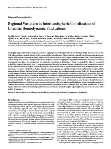
Figure 3. Correlation coefficients between annual-averaged sea surface temperatures (SSTs) and (a) Cool Tongue (CT) index (1903-90), (b) Global Residual (GR) index (1903-90), (c) rotated tropical PC index (1914-90), and (d) North Pacific PC index (1914-90). The contour interval is 0.2, dashed where negative. Correlations greater than +0.2, or less than -0.2, pass a two-tail student-t test of being different from zero at 95% significance levels.
index is more (negatively) correlated with SSTs of the North Pacific. Extratropical SSTs in the southern Pacific are about equally correlated to the two indices. Both indices are modestly correlated with SSTs in the tropical Indian Ocean. Despite the differences in emphasis between the CT and GR correlations, the two most remarkable aspects of the SST patterns associated with the two indices are (1) the symmetry of each correlation pattern about the Equator in the Pacific basin, and (2) the overall similarity between the CT and GR patterns. This similarity led ZWB to describe the decadal variations that dominate the GR index as “decadal ENSO-like variability” and motivated this study. The strong crossequatorial symmetries of the SST patterns are reflected in strong symmetries of atmospheric circulations and hydroclimatic responses analyzed in subsequent sections of this
chapter. The rotated tropical and North Pacific PC indices are correlated to SSTs in patterns (Figs. 3c-d) that are similar to CT and GR, respectively. However, SST correlations with the tropical PCs emphasize the tropical Pacific SSTs (relative to extratropical SSTs) even more than do the CT SST correlations. Seasurface temperature correlations with the North Pacific PCs emphasize the North Pacific temperatures even more than does GR. Once again, southern SSTs are about equally correlated with the two PC series. Thus the two pairs of Pacific climate indices correspond to similar patterns of SST variation. The CT corresponds largely to ENSO variations by its very definition; the tropical PC emphasizes those variations as an outgrowth of the parsimony provided by all PC analyses. As representations of ENSO
8
variations in the tropical Pacific, the CT and tropical PC series have dominantly interannual timescales (Fig. 2). The GR and, even more so, the North Pacific PC series capture variations that are not correlated with CT variations; that are dominantly decadal (although neither has been limited to that timescale; Fig. 2); and that are similar to SST patterns in the world oceans associated with ENSO. How the interannual and decadal climate indices can be related to such similar SST patterns, while having such different (and, in the case of the PCs, entirely uncorrelated) temporal variations, is something of a mystery, but these similarities will be echoed in the atmospheric expressions of the time series as well as in their hydroclimatic expressions over the Americas. Miller and Schneider (1998) recently listed six categories of mechanisms that may contribute to the decadal timescales of SST variations in the North Pacific: • Stochastic atmospheric forcing with a low-frequency SST response (e.g., Barsugli and Battisti 1998) • Decadal tropical forcing of midlatitude SSTs (e.g., Trenberth 1990, Graham 1994) • Decadal midlatitude ocean– atmosphere interactions of ocean gyre strength and wind stress curls (e.g., Latif and Barnett 1994, and, as a North Atlantic analog, Deser and Blackmon 1993) • Tropical–extratropical interactions through subduction of midlatitude (atmospherically forced) SST anomalies into the subsurface ocean to provide source waters of upwelling in the El Niño region of the tropical Pacific (e.g., Gu and Philander 1997) • Slow oceanic-wave teleconnections from the tropics to the extratropical oceans (e.g., Jacobs et al. 1994) • Intrinsic decadal vacillation of
midlatitude ocean currents (e.g., Jiang et al. 1995) To this list, we would add the slow vestiges of irregular interannual ocean–atmosphere climate variations. Aperiodic variations on interannual scales will yield decadal components upon averaging to decadal timescales, and those “decadal” variations will necessarily be similar in appearance to the interannual climate processes. Some combination of these mechanisms, then, presumably generates decadal Pacific SST variations that, in turn, influence and even drive parts of the global climate system with clear, if irregular, decadal timescales. Notably, the present analysis demonstrates remarkable interhemispheric symmetries in expressions of the decadal climate variations associated with the “North Pacific” modes. This interhemispheric symmetry may provide clues as to which of the processes listed above is most likely to be dominant; e.g., those that would be expected to yield strong symmetries about the equator. Resolution of the question of which mechanisms dominate is, however, beyond the scope of the present analysis and will require a careful combination of ocean– atmosphere modeling with careful analyses of the details of global atmospheric and oceanic observations over the last 50 years. Atmospheric associations Superposed on these SST patterns, and interacting with them, are the atmospheric counterparts (and consequences) of the CT and GR SST variations. Regression coefficients relating 500 mb height anomalies (deviations of the heights of 500 mbar pressure surfaces in the atmosphere from their long-term seasonal averages) to the CT and GR series are shown in Figures 4a and 4c. Note that regression coefficients are related to correlation coefficients by
9
(a) CT versus 500-mb heights 0
0 5
0
-15
-5
10
-5
0
5
-1
30 N
0
-10 0 5
5 5
-5
60 N
-1
0
5
5
10 5
-5
60 N
(c) GR versus 500-mb heights
-5
-5
30 N
0
0 5
5 0
0
-5
-5
0
5
30 S
0
30 S
5
-1 0
60 S
5
60 S
180
120 W
60 W
0
0
60 E
(b) CT versus 500-mb storms
0
0
120 E
180
-1.5
120 W
.5
0
-1
0
60 E
-2
60 W
0
0
0.5
30 N
60 E
0 00
0 30 S
.5
00 -0.5
1 0.5
0
-0
0
0
0
0
0 -0.5
0.5
60 N
-0
30 S
.5
-0
0 0
0 0 0.5 1
0
-1
00 00
60 S
60 W
00 1
00
0
0
5
-0.
1 0.5 00
00
-0.5
0-1
0.5
30 N
120 W
(d) GR versus 500-mb storms
-0.5
00
0
180
00
0
-0.5
60 N
120 E
00
120 E
0. 5
60 E
0
0
-1
60 S
0
120 E
180
120 W
60 W
0
Figure 4. Regression coefficients relating (a) 500 mb height anomalies to Cool Tongue (CT) index, (b) 500 mb storminess to CT index, (c) 500 mb height anomalies to Global Residual (GR) index, and (d) 500 mb storminess to GR index. The contour intervals in (a) and (c) are 5 m per climate-index standard deviation, and in (b) and (d) are 0.5 m per climate-index standard deviation. Storminess in panels (b) and (d) is measured by monthly standard deviation of band-pass (3-10 days) filtered 500 mb height anomalies.
β = r σ500 / σclim, where β is a regression coefficient, r is the corresponding correlation coefficient, σ500 is the local standard deviation of 500 mb height anomalies, and σclim is the standard deviation of the climate index. Hence, these maps can be interpreted as the typical atmospheric anomaly that accompanies a modest excursion (1 standard deviation) of the climate index. Negative coefficients relate the 500 mb height anomalies and CT over vast Siberian and North Pacific regions, whereas a northwestsoutheast slanted dipole of positive and negative coefficients is indicated over the South Pacific (Fig. 4a). The negative coefficients correspond to lower than normal 500 mb heights when CT is positive (El
Niños). The broad region of negative coefficients over the North Pacific corresponds to an average 500 mb height decline of as much as 20 m for a 1 standard deviation rise in CT. Positive CTs (El Niños) are associated with deeper than normal Aleutian Lows, and the resulting steep north-south coefficient gradients near 35°N 160°W in Figure 4a correspond to anomalously strong 500 mb height gradients, and anomalously strong westerly winds, when CT is positive. Anomalies in atmospheric circulations associated with positive CT values (El Niños) thus bring storms and precipitation to the southwestern and southeastern parts of North America. The circulation pattern associated with positive CTs also results in enhanced midlatitude blocking and the diversion of
10
storms away from northwestern North America. The effects of these circulation changes on North American climate and hydrology will be discussed in the next section. The dipole of positive and negative coefficients over the southeast Pacific in Figure 4b corresponds to diversions of low pressure systems and attendant storms toward the subtropical belt of South America when CT is positive (El Niños), in a rough parallel to the changes in circulation in the northern hemisphere. Observations of 500 mb heights in the far south are rare enough, however, so that the coefficients may reflect dynamic consistency requirements of the reanalysis process (Kalnay et al. 1996) more than an observed feature of atmosphere. Anomalously strong westerly winds are associated with positive CT along a belt extending from the southern ocean near the international date line to the southern Archipielago de los Chonos of Chile. These patterns have been described as the Pacific South American pattern, a primary mode of Southern Hemisphere atmospheric variability (Mo and Ghil 1987, Kidson 1988, Mo and Higgins 1998, Garreaud and Battisti, 1999). Together, the low-pressure bands (of negative coefficients) associated with positive CT in the Northern and Southern Hemispheres reflect the extratropical extensions of the SOI seesaw of pressures. The Southern Oscillation pattern is not well represented at 500 mb in the tropics (Fig. 4a), but along 30°N and 30°S it appears as the equatorward increase in coefficients (toward positive values in the tropics). In the tropical eastern Pacific, the increase in height at 500 mb is mirrored as a decrease in pressure in the lower troposphere and a slackening of easterly trade winds during El Niños. The relations between CT and midlevel winds and low-pressure systems are inferred from regression coefficients mapped in Figure 4a. Corresponding relations between CT and
storminess can be inferred from regression coefficients relating monthly standard deviations of high-frequency 500 mb height anomalies to CT, as in Figure 4b. Positive values in Figure 4b correspond to regions in which 500 mb heights are more variable, on 3to 10-day timescales, than normal when CT is positive; regions with negative values are less variable and less stormy. Positive CTs (El Niños) are associated with less than normal storminess across Siberia, Alaska, northwestern Canada, and the northwestern United States. By this measure, the southwestern United States is more stormy than normal during El Niños, but the Eastern Pacific storm track, near 35°N 160°W, is clearly enhanced, is extended farther eastward over the southern United States, and is displaced farther south than normal. Storminess may also be enhanced during El Niños over northeastern Canada. A similar analysis (not shown here) of monthly standard deviations of high-frequency SLP variability in the Northern Hemisphere (where daily SLP records span the entire twentieth century) indicates that the associations of SLP-based storminess with CT closely parallels those in the northern half of Figure 4b both before and after the 1950s (the period encompassing the bulk of available 500 mb height observations). In the Southern Hemisphere, positive CTs (El Niños) are associated with greater storminess over the central Pacific along the band from 30° to 50°S. Between South America and the date line, storminess appears to be diverted northward from midlatitudes Less (40° to 60°S) towards about 30°S. storminess is indicated over southern Argentina. The atmospheric expressions of GR are broadly similar to CT’s influences, but—as with SSTs—with different spatial emphases. In Figure 4c, notice that regression coefficients relating 500 mb height anomalies to GR are dominated by negative coefficients over the North Pacific and a weaker north-south dipole
11
of negative and positive coefficients over the South Pacific. The negative coefficients over the North Pacific are very similar to coefficients associated with CT. However, the less similar circulation anomalies over North America indicate that the circulations associated with CT are more zonal than those associated with GR. In the Southern Hemisphere, the dipole of coefficients is much less intense, implying relatively less expression of GR than CT in Southern Hemisphere 500 mb heights and winds. Storminess patterns associated with GR loosely parallel those associated with CT, but variations of GR (Fig. 4d) seem to yield storminess anomalies that are more focused over the North Pacific and the Pacific Northwest, with a much weaker expression over the southern United States than is associated with CT. In the midlatitude Pacific of both hemispheres, the relationship between storminess anomalies and the average 500 mb height anomalies during ENSO variations is similar to the relationship between storminess anomalies and the average 500 mb heights during the decadal ENSO-like variability: A decrease (increase) in storminess is found on the poleward (equatorward) flank of the negative midlatitude height anomaly in the central Pacific (e.g., on the flanks of the Aleutian Low) when the indices are positive. The Northern Hemisphere storminess patterns associated with GR (Fig. 4d) also are reflected in correlations of pre-1950s GR values with SLP-based storminess indices from that earlier period (not shown). Taken together, the panels of Figure 4 suggest qualitative similarities in the atmospheric expression of interannual ENSO variability (CT) and decadal ENSO-like variability (GR). These atmospheric similarities, and the SST similarities discussed previously, will be related to their similar hydroclimatic effects in the Americas in the next section. Overall, the atmospheric expressions of both CT and GR (as well as
tropical and North Pacific PC indices—not shown here) are remarkably symmetric about the Equator, especially over the Pacific Ocean: positive CT and positive GR variations are associated with equatorward diversions of westerlies, low-pressure systems, and storms from the midlatitude Pacific basins toward subtropical latitudes. These cross-equatorial symmetries may reflect tropical roots for both CT and GR (and for the tropical and North Pacific PCs). Thus strong interhemispheric symmetries of ENSO-like variations of Pacific climate are likely to produce strong interhemispheric climate variations along the entire length of the North and South American cordillera on both interannual and decadal timescales.
Climatic effects in the Americas Most of the paleoclimatic records of climate variability studied as parts of PEP-I are proxies for either near-surface temperature variations or precipitation/soil-moisture variations over the Americas. The interannual and decadal ENSO-like climate variations depicted in the previous sections play important roles in determining those variations, roles that will be delineated below. Annual-scale temperature, precipitation, and streamflow variations associated with CT and GR are illustrated in Figure 5, which shows regression coefficients relating deviations of October-September averages of precipitation and temperatures from normal to CT (Figs. 5a and 5c) and GR (Figs. 5d and 5f), respectively. Also shown are correlation coefficients between streamflow and CT (Fig. 5b) and GR (Fig. 5e). Correlations are indicated by circles with radii proportional to the coefficients. Sizing the circles with radii proportional to correlation (and regression) coefficients makes the area of the circles proportional to the fraction of variance that is associated with the climate index at each site.
12
Cool-Tongue index, 1904-90 (a) Precipitation
(b) Streamflow
(c) Temperature
60 N
60 N
30 N
30 N
0 30 S
0 B = -10mm/mon Dry
r = -0.3 Dry
30 S
B = -0.2C Cool
60 S
60 S 135 W
90 W
45 W
135 W
90 W
45 W
135 W
90 W
45 W
Global-Residual index, 1904-90 (d) Precipitation
(e) Streamflow
(f) Temperature
60 N
60 N
30 N
30 N
0 30 S
0 B = +10mm/mon Wet
r = +0.3 Wet
30 S
B = +0.2C Warm
60 S
60 S 135 W
90 W
45 W
135 W
90 W
45 W
135 W
90 W
45 W
Figure 5. Regression coefficients—B—relating Cool Tongue (CT) index to October-September (a) precipitation, 1904-90, and (c) surface-air temperatures, 1904-90; and correlation coefficients—r—between CT and (b) streamflows, periods of record ranging as long as 1904-1990 but commonly on order of 40 years. Panels (d)-(f) are same as (a)-(c) but for Global Residual (GR) index. Radii of circles are proportional to magnitude of regression and correlation coefficients; black for positive relations, white for negative. Circles inset near 30°S, 135°W, indicate scale of influences: B is regression coefficient and r is correlation coefficient (r=0.3 is significantly different from zero at 95% confidence level for average length of streamflow records).
Precipitation and streamflow Strong spatial similarities between CT- and GR-forced patterns of precipitation are immediately obvious from a comparison of Figures 5a and 5d. Streamflow variations with CT and GR also are similar (Figs. 5b and 5e) and mostly reflect, and even amplify (Dettinger et al. 2000), basin-scale
precipitation variations. Both CT and GR are positively correlated with precipitation and streamflow in the southwestern United States, Central America, and in Paraguay, Uruguay, and northern Argentina. Both CT and GR are negatively correlated with precipitation and streamflow in much of northwestern North America, in the tropical parts of South America, east of the Andes, and possibly—
13
although data are particularly sparse there—in southernmost South America. Composite averages (not shown here) of precipitation and streamflow during negative and positive phases of CT and GR indicate that drier than normal conditions in tropical South America and in the northwestern United States are more extreme during positive phases of both CT and GR, and contribute more to the regression relations shown in Figure 5 than do wet conditions during negative CTs and GRs. Positive values of both CT and GR also contribute more (wetness) to the regression relations for the southwestern United States and ParaguayUruguay-Argentina than do negative phases. Negative phases may be more important contributors to the regression relations in the northeastern United States. Dettinger et al. (1998) and Cayan et al. (1998) also found clear similarities between ENSO and decadal precipitation patterns over western North America. In the midlatitudes of the Northern Hemisphere, the precipitation and streamflow patterns shown in Figure 5 reflect the equatorward shifts in midlatitude westerlies and storm track associated with positive values of CT and GR that were indicated in Figure 4 and discussed in the preceding section. When CT is positive, more storms, precipitation, and streamflow occur in the southern United States and, across the equator, in Paraguay-Uruguay; the northwestern United States and much of western Canada States experiences less stormy, drier and warmer conditions. The patterns of precipitation, streamflow, SST, and circulation anomalies over the Americas associated with CT and GR are remarkably similar. However, there are notable differences in spatial emphasis. Precipitation and streamflow anomalies in the tropical parts of South America and in the subtropical bands across North and South America are larger and more consistent (spatially) in the CT responses than in the GR responses (Figs. 5a-b and Figs. 5d-e). Precipitation and, especially, streamflow
responses to GR are larger in northwestern North America, Mexico, and Central America than are the corresponding CT responses. Again, we are struck by the remarkable interhemispheric symmetries of ENSO-like climate variations in the western Americas. As expected from their close ties to CT and GR, regression coefficients relating the rotated PC series (tropical PC and North Pacific PC) to precipitation and streamflow (Figs. 6a-b and 6d-e) are similar to the corresponding patterns for CT and GR. The precipitation and streamflow patterns associated with the two PC series are also remarkably similar to each other, even though the two PCs are uncorrelated time series; the pattern correlation between the precipitation coefficients in Figures 6a and 6d is +0.41 and the pattern correlation between streamflow correlations in Figures 6b and 6e is +0.42. Furthermore, three-fourths of the correlations have the same signs in Figure 6b and 6e. As with CT and GR, positive tropical PC and North Pacific PC excursions are associated with wetter than normal southwestern United States and Paraguay-Uruguay-Patagonia, and drier than normal tropical South America, northwestern North America, and southernmost South America. As with CT and GR, the decadal North Pacific PC is more strongly expressed in northwestern North American precipitation and streamflow variations (and perhaps in southernmost South America) than is the tropical PC, whereas precipitation and streamflow in most other regions more strongly express the tropical PC series. These parallels and connections can also be identified by computing the leading PCs of streamflow and precipitation in the Americas and then correlating the variations of those leading modes with global SSTs (Dettinger et al. 2000) to obtain SST correlation patterns that closely resemble the combined ENSO and decadal ENSO-like SST patterns studied here.
14
Tropical PC index, 1915-88 (a) Precipitation
(b) Streamflow
(c) Temperature
60 N
60 N
30 N
30 N
0 30 S
0 B = -10mm/mon Dry
r = -0.3 Dry
30 S
B = -0.2C Cool
60 S
60 S 135 W
90 W
45 W
135 W
90 W
45 W
135 W
90 W
45 W
North-Pacific PC index, 1915-88 (d) Precipitation
(e) Streamflow
(f) Temperature
60 N
60 N
30 N
30 N
0 30 S
0 B = +10mm/mon Wet
r = +0.3 Wet
30 S
B = +0.2C Warm
60 S
60 S 135 W
90 W
45 W
135 W
90 W
45 W
135 W
90 W
45 W
Figure 6. Same as Figure 5, but for the tropical PC index (a-c) and North Pacific PC index (d-f), 1915-88, respectively.
Surface air temperature Positive CT and GR indices are associated with warmer than normal surface conditions in much of the Americas. The patterns indicated for CT temperatures (Fig. 5c) and GR temperatures (Fig. 5f), however, are not as similar as are the precipitation patterns discussed previously. Positive CTs (El Niños) are associated with warm temperatures in Canada, the western United States, Central America, much of tropical South America (on both sides of the Andes), Paraguay-Uruguay-
Patagonia, and southeasternmost Brazil (see also Diaz and Kiladis 1992). El Niños bring cool temperatures in the southeastern United States and in the eastern Amazon basin. Positive GRs are associated with warmer than normal conditions in northwestern North America and cooler than normal conditions across southeastern and eastern North America. Temperature conditions elsewhere are not as closely related to the GR index as they are to CT. These temperature relations are largely echoed in regression coefficients for the tropical and North Pacific PCs (Figs. 6c, f).
15
As was the case with CT and GR, the spatial patterns of temperature relations with the two PC series are not as similar as are the relations for precipitation and streamflow; the pattern correlation between Figures 6c and 6f is only +0.16. These temperature responses to CT and GR are as expected from the atmospheric circulation changes associated with the two indices. When positive, both CT and GR tend to route anomalously southerly winds over western North America as circulations become more zonal over much of the North Pacific. The winds then tend to be anomalously northward near the west coast of North America from northern Mexico to Alaska (Fig. 4a). Warmer than normal American tropics derive from warmer SSTs and drier conditions in tropical South America (Diaz and Kiladis 1992). In subtropical South America, poleward deviations of the westerlies also result in warmer temperatures overall. Cooler temperatures in the southeastern United States with positive CTs and along the entire eastern United States are consistent with more storminess and anomalously northerly winds there, respectively, as indicated by the details of the 500 mb height regression coefficients shown in Figures 4a and 4b.
Discussion The interannual and decadal ENSO-like variations of the Pacific climate system described here make important contributions to modern climatic and hydrologic variations of the Americas. For example, the numbers of temperature, precipitation, and streamflow series in which various amounts of variance are attributable to a combination of the tropical and North Pacific PCs are summarized in Table 2. Because the PC series are uncorrelated, the percentage of a series variance attributable to them is simply the sum of the square of their respective correlations with the series. More than 30% of the variance is explained by various combinations of the two PC series in over a quarter of all the weather series considered here; almost a third of the temperature series and a fifth of the streamflow series owe half or more of their year-to-year variance to the interannual and decadal ENSOlike climate variations. Perhaps the most important implication of these strong dependences upon the interannual and decadal ENSO-like climate variations is that strong interhemispheric symmetries are to be expected in, at least, temperature, precipitation, and streamflow variations. Other forms of climate variation (e.g., North Atlantic
. Table 2: Percentages of temperature, precipitation, and streamflow series, from sites indicated in Figure 5, with more than threshold fractions of variance explained by the combination of the tropical and North Pacific PC series. Fractions of variance Variance threshold fraction
> 0.2
> 0.3
> 0.4
> 0.5
Temperature
58
42
38
30
Precipitation
35
27
25
14
Streamflow
39
35
30
21
16
climate oscillations) may be distinguishable from the ENSO-like variations simply by their equatorially asymmetric influences on the Americas. Given the important role of these ENSOlike climate variations, a capacity to recognize their variations in paleoclimatic proxies is desirable; reconstructions of these ENSO-like climate variations could form a groundwork for assessing the stability and long-term contributions of the Pacific climate system to the modern climate of the Americas. Given the possibly quite different mechanisms that underlie the interannual and decadal ENSOlike variations, it also would be desirable to reconstruct their separate contributions in paleoclimatic proxies. Separate reconstructions would help us to understand how stable and reliable these important contributors are to modern climate within their differing timescales, in the face of natural and humaninduced climate changes. The interannual and decadal ENSO-like climate variations are influential over large areas of the PEP 1 region, and both affect temperatures, precipitation, streamflow, and (presumably) soil moisture—all of which may be amenable to a variety of paleoclimatic reconstructions. At the same time, however, the interannual and decadal ENSO-like variations may yield spatial patterns of variation of proxies that are difficult to separate from each other. If the analyses of instrumental records presented in previous sections are any indication, it will be difficult to use paleoclimate proxies to distinguish between the two forms of Pacific climate variability from patterns of temperature and, especially, precipitation proxies alone. Indeed, PC analyses of precipitation and streamflow in the Americas (Dettinger et al. 2000) similarly found that interannual and decadal hydroclimatic variations associated with ENSO-like atmospheric forcings could not be separated orthogonally, whereas other, less influential combinations of ENSO-like and
North Atlantic climate variability could be. Perhaps, whether ENSO related or decadal in nature, the similar SST patterns associated with the ENSO-like variations cause such rapid and similar responses from the atmosphere that the particular processes that determine those SST variations matter little to their atmospheric and continental outcomes (e.g., Deser and Blackmon 1993). In that case, it may be exceedingly difficult to be certain which of the ENSO-like climate forces are providing the interannual or decadal fluctuations in North and South American proxies. We have limited this analysis to instrumental records, which span roughly 100 years; careful scrutiny of multiple-series, spatial networks of paleoclimate proxies to determine how commonly the interhemispheric ENSO-like pattern recurs and over what timescales it is present clearly is warranted. The changes in atmospheric circulations and continental climate associated with the ENSO-like climate variations represent temporary reorganizations of distributions of heat and water on global scales. Because of this large scale and because of the strong similarities between the influences of ENSO and decadal ENSO-like climate variations on the Americas, these climate variations also have important effects on the geochemical makeup of the atmosphere. Overall, the positive (El Niño-like) CT and GR forcings are associated with drier tropical conditions in the Americas and mostly wetter extratropical conditions (Figs. 5a-b and 5d-e), along with mostly warmer temperatures (Figs. 5c and 5f); these responses are part of a global pattern of drier tropical lands during El Niño-like periods (Dettinger et al. 2000). On interannual timescales, these influences affect vegetation and surface fluxes of CO2 in ways that are observable on global scales (Siegenthaler 1990; Keeling et al. 1995; Dettinger and Ghil 1998). The strong similarities of effects of interannual ENSO and decadal ENSO-like
17
climate influences in the Americas (and elsewhere) suggest that similar ENSO-like variations of global CO2 concentrations may occur on decadal timescales. Finally, the similarities between the influences of ENSO and decadal ENSO-like climate variations on the Americas, together with their differing timescales, ensures that sometimes CT and GR—and their respective precipitation, streamflow, and temperature patterns—share the same signs and sometime they are in opposition. When the signs of the indices agree, the precipitation, streamflow, and temperature patterns in Figures 5 and 6 can be expected to reinforce each other; when the indices disagree, the patterns may interfere and reduce the overall precipitation, streamflow, and temperature responses. Constructive and destructive influences such as these have been documented by Gershunov and Barnett (1998) and Gershunov et al. (1999) over the United States and results presented here indicate that similar influences can be expected in many other regions of North and South America. Conclusions During the twentieth century, three phenomena have dominated climate variations in the Americas on interannual and decadal timescales. The ENSO phenomenon dominates global climate variations on interannual timescales, and ENSO-like variations over the Pacific Ocean basin and North Atlantic climate variations dominate climate variations on decadal timescales. In this chapter, historical oceanic and atmospheric patterns of climate variability associated with ENSO and ENSOlike variations of the Pacific basin are analyzed and their influences on the temperatures, precipitation, and hydrology of the Americas are compared. Several climate indices that reflect the ENSO interannual and ENSO-like decadal climate variations have been developed in the
literature, including the SOI, Niño-3 temperatures, and the CT index for the tropical ENSO variations, and the PDO index and socalled GR index for decadal ENSO-like variability. In this chapter, another pair of indices is developed on the basis of a PC analysis of SOI, CT, and PDO; the resulting PC series are closely related to CT and GR, but they were not formed by application of explicit temporal filters to separate ENSO and decadal ENSO-like variations (as was GR). By construction, the PC series are completely uncorrelated with each other, to prevent double counting of climate variations when their respective contributions to regional climate variations are compared. The CT and tropical PC indices are two expressions of the tropically based, dominantly interannual climate variations associated with ENSO. Compared to the interannual ENSO signal, the GR and North Pacific PC indices are dominantly decadal and are expressed most fully in the subtropics and midlatitudes of both hemispheres in the Pacific basin. A number of different mechanisms have been described in the literature to explain the decadal character of the extratropical Pacific SST variations— some directly related to ENSO and others not—and no single one of these explanations is preferred by the scientific community at this time; see the section on Sea-Surface Temperatures earlier in this chapter for some examples of the alternatives under consideration. At the 500 mbar level in the atmosphere (about 5 km above sea level), positive phases of the CT and GR, and their counterpart PC series, are associated with anomalously low heights (pressures) over the North Pacific at the climatological position of the Aleutian Low, stronger westerly winds, and southward diversion of westerlies and storminess across the North Pacific basin. In the tropics, CT is associated with the entire suite of ENSO teleconnections and atmospheric changes; GR is not expressed so clearly in the tropics (as
18
gauged by SSTs there). In the Southern Hemisphere, positive CT and GR, and PCs, are associated with a dipole of 500 mb height anomalies that also shifts westerlies and storminess equatorward. The spatial patterns of 500 mb height anomalies associated with CT and GR are remarkably similar, reflecting the qualitative similarities in SST patterns associated with the indices, despite their differing time series. The patterns of atmospheric circulation changes associated with the indices also are remarkably symmetric about the Equator in the Pacific sector. Over North and South America, the similarities of the spatial distributions of climatic forcings associated with the interannual and decadal ENSO-like variations of the Pacific basin result in similar precipitation and streamflow patterns that are basically symmetric about the Equator in the western Americas, on both interannual and decadal timescales. The interannual and decadal ENSO-like patterns of precipitation and streamflow also are similar to each other overall, although more differences arise when the precipitation associations with the tropical PC and North Pacific PC (which are by design completely uncorrelated) rather than with CT and GR (which are share some variability) are considered. Surface air temperature patterns associated with the ENSO-like climate forcings may be somewhat less spatially similar from timescale to timescale. Wetter than normal conditions accompany positive phases of CT (El Niños) and GR in the subtropical belts of both continents; drier than normal conditions accompany them in much of tropical South America (east of the Andes) and in the midlatitudes of the northwestern United States and perhaps in southernmost South America. At the hemispheric scale, positive phases of the CT (El Niños) and GR indices historically have resulted in more consistent and stronger precipitation and streamflow responses in the Americas than have negative
phases, except in the same midlatitude belts of the two continents. Temperatures in the Americas have tended to be warmer overall during positive phases of both CT and GR, except across the southeastern United States, eastern United States (for GR), and parts of the Amazon basin. Together the interannual and decadal ENSO-like climate variations are related to more than half the year-to-year variance in one-third to one-fifth of the temperature and streamflow series analyzed here. Present understanding of the processes leaves open the possibility that the interannual and decadal SST variations derive from very different physical processes with different timescales and different vulnerabilities to long-term natural and human-induced changes. The atmospheric variations and climatic consequences for the Americas that are associated with the interannual and decadal SST variations may derive from quick physical responses to overall SST variation that depend relatively little upon which SST process is dominant. Even if the atmosphere and continents prove to be slavish in their responses to SST variations, regardless of the source of those variations, the climatic consequences still would reflect the different vulnerabilities to change of the various SST processes. Thus, improved understanding of the processes represented by CT and GR should be a high priority for present-climate, paleoclimate, and climate-change researchers. It is unfortunate, then, that the strong spatial similarities between the hydroclimatic outcomes of historical ENSO-like climate variations will probably impede most efforts to reconstruct, separately, these two dominant modes of climate variation in the Pacific basin by paleoclimatic proxies from the Americas. The results presented here, however, compare ENSO-like SST and climate variations; other modes of SST and climate variation may be important in many locales and may be easier to distinguish from ENSO and ENSO-like
19
behavior of the global climate system. Finally, because this analysis is restricted to variations during the last century, the amplitude of the SST variations at work is only a few degrees large. Extrapolation to the larger SST anomalies of past climates would be speculative and, indeed, even the close spatial similarities of ENSO and decadal ENSO-like climate variations found here may break down under larger SST forcings or under changing mean temperature conditions of the distant past. Acknowledgments We are very grateful to Vera Markgraf for organizing and shepherding the PEP-I Workshop in Merida, Venezuela; it was a remarkably informative and useful week. Discussions with Dave Enfield, of the National Oceanic and Atmospheric Administration (NOAA) and the Atlantic Oceanographic and Meteorological Laboratory; Jose Marengo, Instituto Nacional de Pesquisas Espacias; and Henry Diaz, NOAA Climate Diagnostics Center, contributed to the ideas developed here. Comments by Dan Cayan, Scripps Institution of Oceanography, and Michael Evans, Lamont-Doherty Earth Observatory, greatly improved this chapter. Access to streamflow, precipitation, and temperature data provided by Dan Cayan and Larry Riddle at Scripps Institution of Oceanography; to Brazilian streamflow series made available by Jose Marengo, courtesy of Eletrobras and Eletronorte; and to 1948-1958 daily 500 mbar height fields by Wayne Higgins of the NOAA Climate Prediction Center made parts of this analysis possible. In addition to National Science Foundation’s funding for the workshop as a whole, MDD’s efforts were supported by the U.S. Geological Survey’s Global Change Hydrology Program and DSB’s efforts were supported by grants from NOAA’s Office of Global Programs.
References Allan, R., J. Lindesay, and D. Parker, 1996: El Niño, Southern Oscillation and Climate Variability. Collingwood, Australia: CSIRO Publishing, 405 p. Barsugli, J.J., and D.S. Battisti, 1998: The basic effects of atmospheric-ocean thermal coupling on midlatitude variability. Journal of the Atmospheric Sciences,
55:477-493. Bitz, C.M., and D.S. Battisti, 1999: Interannual to decadal variability and the glacier mass balance in Washington, Western Canada, and Alaska. Journal of Climate, 12:3181-3196. Cayan, D.R., M.D. Dettinger, H.F. Diaz, and N. Graham, 1998: Decadal variability of precipitation over western North America. Journal of Climate, 11:3148-3166. Deser, C., and M. Blackmon, 1993: Surface climate variations over the North Atlantic Ocean during winter: 1900-1989. Journal of Climate, 6:1743-1753. Deser, C., and J.M. Wallace, 1990: Large-scale atmospheric circulation features of warm and cold episodes in the tropical Pacific. Journal of Climate, 3:1254-1281. Dettinger, M.D., and H.F. Diaz, submitted: Global characteristics of streamflow seasonality and variability. Journal of Hydrometeorology. Dettinger, M.D., and M. Ghil, 1998: Seasonal and interannual variations of atmospheric CO2 and climate. Tellus, 50B:1-24. Dettinger, M.D., D.R. Cayan, H.F. Diaz, and D. Meko, 1998: North-south precipitation patterns in western North America on interannual-to-decadal time scales: Journal of Climate, 11:3095-3111. Dettinger, M.D., D.R. Cayan, G.J. McCabe, and J.A. Marengo, 2000: Multiscale hydrologic variability associated with El Niño/Southern Oscillation. In Diaz, H.F., and V. Markgraf (eds.), El Niño and the Southern Oscillation--Multiscale Variability, Global and Regional Impacts. Cambridge: Cambridge University Press, 113-146. Diaz, H.F., and G.N. Kiladis, 1992: Atmospheric teleconnections associated with the extreme phases of the Southern Oscillation. In Diaz, H.F. and V. Markgraf (eds.), El Niño: Historical and paleoclimatic aspects of the Southern Oscillation. Cambridge: Cambridge University Press, 7-28. Diaz, H.F., and V. Markgraf (eds.), 1992: El Niño: Historical and paleoclimatic aspects of the Southern Oscillation. Cambridge: Cambridge University Press, 476 p. Ebbesmeyer, C.C., D.R. Cayan, D.R. McClain, F.H. Nichols, D.H. Peterson, and K.T. Redmond, 1991: 1976 step in the Pacific climate: Forty environmental changes between 1968-75 and 1977-84. Proceedings of the 7th Annual Pacific Climate (PACLIM) Workshop, California Department of Water Resources, 115-126. Eischeid, J.K., C.B. Baker, T.R. Karl, and H.F. Diaz, 1995: The quality control of long-term climatological data using objective data analysis. Journal of Applied Meteorology, 34:2787-2795.
20
Eischeid, J.K., H.F. Diaz, R.S. Bradley, and J.D. Jones, 1991: A comprehensive precipitation data set for global land areas. DOE/ER-69017T-H1, TR051, 81 p. Enfield, D.B., and A.M. Mestas-Nunez, 2000: Interannual to multidecadal climate variability and its relationship to global sea-surface temperatures. In Markgraf, V. (ed.), Present and Past Interhemispheric Climate Linkages in the Americas and Their Societal Effects. San Diego: Academic Press, this volume. Folland, C.K., and D.E. Parker, 1990: Observed variations of sea surface temperature. In Schlesinger, M.E. (ed.), Climate-Ocean Interaction. New York: Kluwer, 21-52. Folland, C.K., and D.E. Parker, 1995: Correction of instrumental biases in historical sea surface temperature data. Quarterly Journal of the Royal Meteorological Society, 121:319-367. Garreaud, R.D., and D.S. Battisti, 1999: Interannual and interdecadal variability in the southern Hemisphere. Journal of Climate, 12:2113-2123. Gershunov, A., and T.P. Barnett, 1998: Interdecadal modulation of ENSO teleconnections. Bulletin of the American Meteorological Society, 79:2715-2725. Gershunov, A., T.P. Barnett, and D.R. Cayan, 1999: North Pacific interdecadal oscillation seen as factor in ENSO-related North American climate anomalies. Eos (Transactions of the American Geophysical Union), 80:25, 29, 30. Graham, N.E., 1994: Decadal scale variability in the 1970’s and 1980’s: Observations and model results. Climate Dynamics, 10:135-162. Gu, D.F., and S.G.H. Philander, 1997: Interdecadal climate fluctuations that depend on exchanges between the tropics and extratropics. Science, 275:805-807. Hurrell, J. W., 1995: Decadal trends in the North Atlantic Oscillation: Regional temperatures and precipitation. Science, 269:676-679. Jacobs, G.A., H.E. Hurlburt, J.C. Kindle, E.J. Metzger, J.L. Mitchell, W.J. Teague, and A.J. Wallcraft, 1994: Decadal-scale trans-Pacific propagation and warming effects of an El Niño anomaly. Nature, 370:360-363. Jiang, S., F.F. Jin, and M. Ghil, 1995: Multiple equilibria, periodic and aperiodic solutions in a winddriven, double-gyre, shallow-water model. Journal of Physical Oceanography, 25:764-786. Jones, P.D., S.C.B. Raper, R.S. Bradley, H.F. Diaz, P.M. Kelly, and T.M.L. Wigley, 1986a: Northern Hemisphere surface air temperature variations: 18511984. Journal of Climate and Applied Meteorology, 25:161-179. Jones, P.D., S.C.B. Raper, and T.M.L. Wigley, 1986b: Southern Hemisphere surface air temperature variations: 1851-1984. Journal of Climate and Applied
Meteorology, 25:1213-1230. Kalnay, E., M. Kanamitzu, R. Kistler, W. Collins, D. Deaven, L. Gandin, M. Iredelli, S. Saha, G. White, J. Woolen, Y. Zhu, M. Chelliah, W. Ebisuzaki, W. Higgins, J. Janowiak, K. Mo, C. Ropelewski, J. Wang, A. Leetmaa, R. Reynolds, R. Jenne, and D. Joseph, 1996: The NCEP/NCAR Reanalysis Project. Bulletin of the American Meteorological Society, 77:437-471. Keeling, C.D., T.P. Whorf, M. Wahlen, and J. van der Plicht, 1995: Interannual extremes in the rate of rise of atmospheric carbon dioxide since 1980. Nature, 375:666-670. Kidson, J.W., 1988: Interannual variations in the Southern Hemisphere circulation. Journal of Climate, 1:1177-1198. Latif, M., and T.P. Barnett, 1994: Causes of decadal climate variability over the North Pacific and North America. Science, 266:634-637. Lees, J., and J. Park, 1995: Multiple-taper spectral analysis: A stand-alone C subroutine. Computers and Geosciences, 21:199-236. Mann, M.E., and J.M. Lees, 1996: Robust estimation of background noise and signal detection in climatic time series. Climatic Change, 33:409-445. Mantua, N.J., S.R. Hare, Y. Zhang, J.M. Wallace, and R.C. Francis, 1997: A Pacific interdecadal climate oscillation with impacts on salmon production. Bulletin of the American Meteorological Society, 78:1069-1079. Miller, A.J., and N. Schneider, 1998: Interpreting the observed patterns of Pacific Ocean decadal variations. In G. Holloway, P. Muller, and D. Henderson (eds.), Biotic Impacts of Extratropical Climate Variability in the Pacific. Proceedings of the Aha Huliko’a Hawaiian Winter Workshop, University of Hawaii at Manoa, 1927. Mo, K.C., and M. Ghil, 1987: Statistics and dynamics of persistent anomalies. Journal of the Atmospheric Sciences, 44:877-901. Mo, K.C., and R.W. Higgins, 1998: The Pacific South American modes and the tropical intraseasonal oscillation. Monthly Weather Review, 126:1581-1596. Percival, D.B., and A.T. Walden, 1993: Spectral analysis for physical applications—Multitaper and conventional univariate techniques. Cambridge: Cambridge University Press, 580 p. Richman, M.B., 1986: Rotation of principal components. International Journal of Climatology, 6:293-335. Siegnthaler, U., 1990: El Niño and atmospheric CO2. Nature, 345:295-296. Slack, J. R., and J.M. Landwehr, 1992: Hydro-climatic data network (HCDN): A U.S. Geological Survey streamflow data set for the United States for the study
21
of climate variations, 1874-1988. U.S. Geological Survey Open-File Report 92-129, 193 p. Trenberth, K.E., 1990: Recent observed interdecadal climate changes in the Northern Hemisphere. Bulletin of the American Meteorological Society, 71:988-993. Trenberth, K.E., and D.A. Paolino, 1980: The northern hemisphere sea-level pressure data set trends, errors, and discontinuities. Monthly Weather Review, 108:855-872. Troup, A. J., 1965: The ‘southern oscillation’. Quarterly Journal of the Royal Meteorological Society, 91: 490506. Wallace, J.M., E.M. Rasmusson, T.P. Mitchell, V.E. Kousky, E.S. Sarachik, and H. Storch, 1997: On the structure and evolution of ENSO-related climate variability in the tropical Pacific: Lessons from TOGA. Journal of Geophysical Research, 103:1424114259. Zhang, Y., J.M. Wallace, and D.S. Battisti, 1997: ENSOlike interdecadal variability: 1900-93. Journal of Climate, 10:1004-1020.
22