Manuscript preparation was supported by the Owen-Coates Fund of the Geology ... 1993, Edwards aquifer storage assessment, Kinney County to Hays County ...
82
Karst Modeling
Halihan, Sharp and Mace
Karst Waters Institute Special Publication 5
\
INTERPRETING FLOW USING PERMEABILITY AT MULTIPLE SCALES Todd Halihana, John M. Sharp, Jr. 0 , and Robert E. Mace!' aDepartment of Geological Sciences, The University of Texas at Austin, Mail Code C1100 Austin, TX 78712 bBureau ofEconomic Geology, The University of Texas at Austin, University Station, Box X Austin, TX 78713 Abstract Two difficulties that karst aquifers can present are permeability that varies with the scale ofmeasurement (up to nine orders of magnitude), and permeability that is so high that standard pump tests obtain no measurable drawdown. Though it is difficult to quantify, permeability is the most sensitive parameter for either laminar or turbulent groundwater equations and must be accurately estimated. Permeability data at the small-scale (laboratory and outcrop) were used to reproduce permeabilities measured at the well- and regional-scales in the San Antonio segment of the Edwards aquifer. These calculations provided an understanding of how features observed at the small-scale affect permeability measurements at larger scales. Conversely, these calculations can be performed on the well- and regional-scale to estimate what small-scale features are influencing the aquifer.ln this paper, equations and techniques are presented to help answer questions such as: ( 1) How can small-scale data be combined to determine an effective well- or regional-scale permeability? (2) What size high-permeability features are influencing an aquifer on the well- or regional-scale? (3) Is the flow in an aquifer Darcian? (4) What velocities should be expected in an aquifer?
effect. There are also short sections explaining the concept of permeability combination modeling and its application to the San Antonio segment of the Edwards aquifer. Finally, equations are presented with examples to aid in understanding how standard hydrogeologic measurements of permeability are affected by the high-permeability features present in karst aquifers for matrix, fracture, and conduit combinations.
Permeability scale effect Kiraly (1975) first mentioned the scale effect in karst aquifers of Switzerland, in which permeability continually increased from the small- to the regional-scale (Figure I). He hypothesized that the increase from small- to well-scale was caused by fractures, and that the largest permeabilities on the regional-scale were caused by karstic conduits. Quinlan and others ( 1992) compiled over 1800 dye traces from 25 countries, and concluded that average flow velocity values continually increased with scale. Extending the work of Brace (1984). Clauser (1992) noted that permeability increased approximately three orders of magnitude from the small-scale to the well-scale in crystalline rocks. However. Clauser suggested that the permeability offractured media measured on the well-scale would not continue to increase when measured on the regional-scale. Other authors have also suggested that if a
Introduction This paper is broken up into sections that may be digested separately. There are various combinations of highpermeability features, and usually someone is interested in certain combinations. Unfortunately, this format may make the paper as a whole somewhat segmented. A longer discussion of how these techniques may be applied to answer specific questions in a fractured karst aquifer can be found in Halihan et al. (in press). The averaging and inversion techniques presented are useful "back of the envelope" calculations which can be used to estimate the effects and dimensions of high-permeability features in karst aquifers. Some definitions are provided for those who are not familiar with karst hydrogeology (Appendix A), and a section is devoted to explaining the permeability scale
PERMEABILITY SCALES •laboratory permeability · core or chip samples •fracture measurements •conduit measurements
•specific capacity tests •drawdown tests
•packer tests
+- small-seal~ +---
welf·scale---t>
•regional modeling •hydrograph analysis
•cave maps
+--
regional-scale-+
Figure 1: Permeability or intrinsic permeability measurements made on different scales. Over this range, aquifer permeability measurements can vary over nine orders of magnitude (Halihan et al., in press). The figure does not include micro-scale measurements of permeability performed in thin sections.
\
Halihan, Sharp and Mace
Karst Modeling Karst Waters institute Special Publication 5
sufficiently large volume of rock was selected, a single, representative value for permeability could be determined (Long and others, 1982; Odling, 1997). Rovey (1994) examined carbonate aquifer permeability with variogram models; he found that for fractured unkarstified carbonates, a range could be determined in which the permeability reached a constant value. But for mature, well-developed karst aquifers, he suggested that permeability increased to "practical infmity ." Halihan eta!. (in press) tested Kiraly's (1975) hypothesis using a permeability database for the San Antonio segment of the Edwards aquifer of central Texas and found that Kiraly's hypothesis was applicable for that aquifer.
10 1
10~
Regional-scale
N
____.
.........
3 studies
10"9
83
~_..
1
o·2 til
E
E
>.
10 5
§ 10·12
.0
:::-
:~
u::>
E
-o c:
a..
u
~
0
10 ·8
10 ·15
Small-scale permeability distributions Small-scale permeabilities in carbonate aquifers have a few common trends. Published matrix permeabilities tend to lie in the range of 5x 1o·" to 5xl 0• 13 m 2 for limestone and dolomite (Freeze and Cherry, 1979). These values can extend from below 1o-l? m2' where they become difficult to measure, up to values of I o·'' m 2, which may include some small solutional voids or fractures (Hovorka et al., 1993; Hovorka et al., 1995) (Figure 2). The permeability of the matrix is often log-normally distributed (Halihan et al., in press), as it is for many lithologies. Fracture permeabilities are highly variable in aquifers. However, the distribution of apertures is generally assumed to follow a log-normal or power-law distribution (Bianchi and Snow, 1969; Barton and Zoback, 1992; Marrett, 1996). When the log-normal or power-law distribution is modified to permeability using the cubic Jaw (Lamb, 1932), generally a single fracture or a small number of fractures will dominate the flow. Although thousands of fractures may be present, the distribution of apertures indicates that only a few will control the aquifer.
0
N
0
M
0
"'
0 0 0 Ll) "-CO
o
L">
ooolll r-- o;) 0> 0>
cr>
0>
Percent
Figure 3: Small-scale permeability information for the San Antonio segment of the Edwards aquifer. The upper diagram is a digital outcrop interpretation of the Lake Medina outcrop that provides the basis for some of the data in the graphical lower diagram. Graphical data compiled from 493 matrix permeability measurements from l-inch cores (Hovorka et a!., 1993; Hovorka et a!., 1995; Hovorka, personal communication), 776 fracture aperture measurements from roadcuts (Hovorka et al., 1998), and 2685 conduit measurements from roadcuts (Hovorka et a!., 1995). Fracture permeability was calculated using equation (4a). Laminar and turbulent conduit permeability was calculated using equations (7c) and (7e), respectively. It is assumed that a homogenous aquifer would yield a straight horizontal line on the diagram.
outcrop. The study illustrated the difficulty in applying standard pump tests to a fractured carbonate aquifer due to the limitations of pumping tests, and the highly heterogeneous nature of the high permeability features in the aquifer.
Permeability combination models Permeability combination models provide a method for performing estimates of 1) averaged permeabilities caused
Percent
Figure 4: Permeability scale effect (thin lines, and points connected with lines; see Figure 2) and permeability combination models (thick lines, and individual points) for the San Antonio segment of the Edwards aquifer. Permeability combination model is shown for a 50-fracture Monte Carlo model using the distributions for matrix and fracture permeability (Figure 3) and equation 6. 2D singleconduit models are shown for laminar and turbulent flow using the distributions for matrix and conduit permeability (Figure 2) and equation 7a. 3D conduit model calculation (individual points) shown for !-meter laminar and turbulent models using equation (8b) with km = 1Q· 11 m", and A = 1.7x10⁶ m2.
by a mixture of different permeable features in an aquifer (Ha1ihan eta!., in press; Figures 3 and 4 ), or 2) size of smallscale permeable features from well- or regional-scale permeability data. These models are steady-state geometric models that estimate the effects of different heterogeneities on aquifer permeability. The models assume that measurements of permeability on different scales are all valid estimates, which simply average different heterogeneities. Permeability combination models are modifications of .equations for layered aquifers (Leonards, 1962; Fetter, 1994). ln addition to the assumptions used for layered aquifers, three additional assumptions are necessary for these models: (1) the hydraulic gradients used in the estimates are uniform between different heterogeneities (2) equation 4g is valid for fractures and equations 7d and 7f are valid for laminar and turbulent flow in conduits; (3) there are no strong interactions between regions with different permeabilities. While the standard techniques for
Holihan, Sharp and Mace
Karst Modeling Karst U'aters Institute Special Publication 5
85
measuring penneability yield average values that generally underestimate flow velocities, these model estimates will likely overestimate flow velocities. These calculations are approximations and are highly dependent on the orientations of the penneable features.
In order to illustrate the use ofthese models, three cases are given for matrix, fracture and conduit combinations with example problems. For combining regions of varying matrix penneability, one case is given for combining smallscale measurements, and two cases for inverting well- or regional-scale measurements. For combinations of fractures and matrix, two cases discuss how to combine small-scale data to obtain estimates of larger-scale permeabilities, and one case illustrating how to estimate fracture aperture from well data. Finally, two cases are presented to estimate how a conduit flowing under laminar or turbulent conditions would affect well- or regional-scale estimates, and one illustrating the problem of estimating conduit size from regional models. The problems are simplified and ask some rhetorical questions, but do illustrate the basic ways in which the high-penneability features present on the small-scale in aquifers can be combined to affect measurements at larger scales. A more formal derivation ofthe equations is presented for the case of a single fracture intercepting a well (case 4).
Figure 5: High-penneability matrix layer located in a lower-penneability aquifer. See Case 1, 2, and 3.
Conductivity:
K =K +(K e
m
/ugh
-K )( bhigh) m b
I b)
101al
Transmissivity:
Case 2: Inverting pump-test results to find highpermeability layer size
Matrix How thick would a high-penneability layer in an aquifer need to be to supply the water flowing to a well? How high would be the permeability detected in a well if it intercepts a known high-permeability zone? What is the penneability of a conductive zone that was encountered during drilling? How much faster does water move through the highpermeability zone than the rest of the aquifer? Often, the permeability of a given lithology is known, or can be estimated using small-scale measurements. Using the small-scale data and infonnation about the well, these questions can be answered with the equations and examples provided (Figure 5) .
Need: (1) transmissivity from pump test (T,); (2) conductivity ofthe two lithologies (K.,, Kh.gh); (3) thickness of aquifer (b 101) . Calculation: (2a)
Approximation: If Tm arctan (b,orar I 2r..), we obtain (Figure 7b):
ke =k +(k -k ) m
(12k) 112
m 1tr
j
f
w
sin(8)
(4k)
Approximation:
3.46(/c_r)312 1trwsin(8)
(41)
In the limit of the high-angle case, for a vertical fractu re (8
= 90°), we obtain: ke =k +(k -k ) m
j
m
( 12k\ 112 jJ
1tr w
Calculate k for the problem using equation 4g: 1
k1 = bf/12 = (1x10 4 m) 2 /l 2 = 8.33x10·10 m=
(a) 8 = 0°, using equation 4h: k, = 1o·I S m= + (8.33xi0· 10 m2 - 10·15 m2)[ 104 m I 10m* cos (0) ]; k, = 10· 1 ~ m=.... (8.33x 10·10 m2 * lxl o·5); k. = 9.33x1 0•15 m2 --an increase of nearly an order of magnitude over the matrix value
Approximation using equation 4i: k, "' ( 3.46 * (8.33xl0·10 m2)3 2 /10 m = 8.32xl0· 1" m3 /10m = 8.32xJ0·15 m2 (b) 8 = 45°: k = l.28xJ0·1< m= --an increase of0.4 times • over the horizontal case. (c) 8 = 75°: ke = 3.32xl0"14 m= -- an increase of2.6 times over the horizontal case. (d) 8 = 90°, using equation 4k: k. = 10.:~ m=- (8.33xi0· 10 m2 - I0·15 m2)[ 104 m I 3.14* 0.1 m *sin (90) ]; k, = 2.66 x 10·13 m2 -- increase of 2 7. 5 times over the horizontal case.
If km