Quantitative Feedback Theory (QFT), is a frequency-domain-based robust control design approach that was developed in the early. 1970s and has received ...
Control Engineering Practice 6 (1998) 805—828
Introduction to Quantitative Feedback Theory for lateral robust flight control systems design S.-F. Wu, M.J. Grimble*, S.G. Breslin Industrial Control Centre, Department of Electronic and Electrical Engineering, University of Strathclyde, 50 George Street, Glasgow G1, 1QE, Scotland, UK
Abstract Quantitative Feedback Theory (QFT), is a frequency-domain-based robust control design approach that was developed in the early 1970s and has received considerable attention over the past two decades. In the last few years, its application to aircraft flight control systems design has been widely investigated. In this paper the basic concepts, principles, design procedure, and features of QFT are reviewed and summarized for single-input single-output systems. Its application to a lateral flight control system design is then considered. A robust roll-attitude control system is designed to cover a certain operating range using the QFT methodology, and certain eigenstructure-assignment results. The integration of QFT with eigenstructure methods results in a controller with the stability and performance robustness of QFT design, and the decoupled dynamic responses of an eigenstructure-assignment approach. The results indicate QFT has significant potential in robust flight control systems design. The combination of techniques should be applicable to other industrial sectors. ( 1998 Published by Elsevier Science Ltd. All rights reserved. Keywords: Control design; frequency domain; QFT; robustness; tracking
1. Introduction Robust control techniques are particularly useful for the design of aircraft flight control systems, partly because aircraft dynamics vary substantially throughout the flight envelope. Variables such as airspeed, flight altitude, fuel consumption, and the amount and location of payload can have a dramatic effect on the aircraft’s plant parameters and on the plant model structure. The variations in the aircraft model can be taken into account through the robustness of the design. One approach to designing robust control systems is through the use of Quantitative Feedback Theory (QFT), which was developed by Isaac M. Horowitz in the early 1970s and has attracted considerable interest over the last two decades (Horowitz and Sidi, 1972; Horowitz, 1976; Houpis, 1987; D’Azzo and Houpis, 1988; Horowitz, 1993; Azvine and Wynne, 1992; Ballance, 1996). This is a frequency-domain-based design technique where the
*Corresponding author. Tel.: 44 141 552 4400; fax: 44 141 548 4203; e-mail: m.grimble.eee.strath.ac.uk.
controllers can be obtained to satisfy a set of performance and stability objectives over a given range of plant parameter uncertainty. The QFT technique (unlike H = and LQG control) is based on the classical idea of frequency-domain shaping of the open-loop transfer function (Breslin and Grimble, 1996). It also differs in the way in which uncertainties are characterized. In QFT design, the uncertainty in the plant gain and phase is represented as a template on the Nichols chart. This template is then used to define regions in the frequency domain where the open-loop frequency response must lie. This is in order to satisfy performance and stability specifications for the entire plant set represented by the uncertainty. The inclusion of phase uncertainty makes it possible to achieve less conservative solutions than those which would be obtained from synthesis procedures such as H design that = are based on gain uncertainty descriptions (Grimble, 1994). This is of course also true of the so called ksynthesis methods. The QFT technique has been applied successfully to many classes of linear problems including multi-input single-output (MISO Horowitz and Sidi, 1972) and multi-input multi-output (MIMO Houpis, 1987; D’Azzo
0967-0661/98/$ — See front matter ( 1998 Published by Elsevier Science Ltd. All rights reserved PII: S 0 9 6 7 - 0 6 6 1 ( 9 8 ) 0 0 0 5 3 - 7
806
S.-F. Wu et al./Control Engineering Practice 6 (1998) 805—828
and Houpis, 1988; Horowitz, 1993) plants, and to various classes of nonlinear and time-varying problems (Horowitz, 1976). Attention here will focus on the scalar linear control design problem. In the last ten years, the application of QFT to flight-control systems design has been studied extensively (Phillips, 1994; Keating et al., 1995; Reynolds et al., 1996; Bossert, 1994; Fontenrose and Hall, 1996; Snell and Stout, 1996; Breslin and Grimble, 1996(a); Breslin and Grimble, 1996(b)). Much of this flight-control research was supported by the Flight Dynamics Laboratory of the Wright-Patterson Air Force Base in Dayton, Ohio (Phillips, 1994; Keating et al., 1995; Reynolds et al., 1996). The research at these labs culminated in the design and the first successful flight testing of a QFT flight-control system in 1992 (Bossert, 1994; Fontenrose and Hall, 1996; Snell and Stout, 1996; Breslin and Grimble, 1996(a); Breslin and Grimble, 1996(b) ). The QFT approach will be shown to be successful in enhancing the robust stability and tracking performance of a lateral flight-control system which was designed previously via a multivariable eigenstructure-assignment approach. The QFT design results are combined below with the eigenstructure-assignment results, to obtain a controller that has the desired robust stability, performance and decoupled dynamic responses. The eigenstructureassignment design process for a lateral flight-control system is described in Wu (1996). Attention is concentrated on the single-input single-output case, but multi-input multi-output problems can be treated in a related manner and nonlinear systems design is a subject of current research. The current intense interest in QFT is partly a result of the availability of good software tools and the availability of significant desktop computing power. The method, without such support (as in the early 70s), was quite unwieldy but it is now very straightforward to use. The paper is organized as follows. The main features and characteristics of QFT are reviewed in Section 2. The lateral flight-control system and its plant uncertainties are summarized in Section 3. Detailed QFT analysis and design for the roll-attitude control system, for given performance specifications, are described in Section 4. Section 5 incorporates the QFT design results within the eigenstructure-assignment solution to obtain the desired controller. Conclusions are then drawn in Section 6.
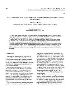
2. Quantitative Feedback Theory In the present context, robust control refers to the design of a controller that causes the output of a system to follow some desired response in a specified manner in the presence of plant parameter variations and/or unwanted and unmeasurable disturbances. The QFT method is a robust control design technique that uses feedback of measurable plant outputs to generate an acceptable response from a system in the face of disturbance signals (Grimble, 1988) and plant modelling uncertainty (caused by full envelope operation). The QFT approach was developed by Professor Isaac Horowitz in the early 1970s but modifications and improvements continue to be made. QFT employs a two degree-of-freedom control structure (providing freedom to shape the feedback and tracking responses independently). This uses unity feedback, a cascade compensator G(s), and a prefilter F(s) to reduce the variations of the plant output due to plant parameter variations and disturbances, as shown in Fig. 1. The QFT method takes into account quantitative information on the plant’s variability, the robust performance requirements, control performance specifications, the expected disturbance amplitude, and attenuation requirements. The feedback loop compensator is designed to ensure that the robustness and disturbance-rejection requirements can be met. The prefilter is then used to tailor the responses to meet the tracking specification requirements. The QFT designs are undertaken using a Nichols chart. Because a whole set of plants rather than a single plant is considered, the magnitude and phase of the plants, at each frequency, yields a set of points on the Nichols chart, instead of a single point. Thus, at each selected frequency a connected region, or so called template, is constructed, which encloses this set of points. Larger templates indicate greater uncertainty; to avoid unnecessary conservatism, the template is usually chosen to be the smallest convex polygon enclosing all of the points. QFT is a transparent frequency-domain design technique in that the trade-offs between compensator complexity and performance are readily visualized, whilst at the same time structured uncertainty is also addressed. Structured plant uncertainty is embodied in a set of
Fig. 1. Canonical two degree-of-freedom feedback structure.
S.-F. Wu et al./Control Engineering Practice 6 (1998) 805—828
two-dimensional magnitude-phase templates that correspond to a set of fixed frequencies, as described above. These templates are then used to define regions (or so called bounds) in the frequency domain, where the openloop frequency response must lie (in order to satisfy the performance and stability specifications, and the disturbance-rejection requirements for the entire plant set). Stability bounds are calculated using these templates and the phase margin. The performance bounds are derived using the templates and upper and lower limits on the frequency-domain response. The disturbance bounds are based on the templates and the upper limit only. The compensator is determined through a loop-shaping process using a Nichols chart that displays the phase and gain margins, stability bounds, performance bounds, and disturbance-rejection bounds. The disturbance-rejection and tracking action of the compensator is based on keeping the loop-transfer gain above the disturbance and tracking bounds on the Nichols chart. During the loop shaping process, modification of the poles and zeros of the compensator produces transparent results, enabling the designer to examine the trade-offs between compensator complexity (order) and system performance. The prefilter design is conducted using a Bode diagram to shape the closed-loop frequency response, so as to satisfy the tracking performance requirement. 2.1. Design procedure The QFT design approach consists of a number of distinct steps, which can be summarized as follows: 1. System formulation The control system to be designed is configured in the form of Fig. 1, with a single feedback loop and a two degrees-of-freedom solution. The dynamic models of the plant are represented by a series of linear time invariant (LTI) transfer-functions over a desired operating range. 2. Design specifications The design specification involves the requirements on the dynamic and steady-state performance of the closedloop system. The specification can be defined in the time-domain using familiar figures such as the rise time t , settling time t and maximum peak overshoot M , or r s p directly in the frequency domain. If time-domain specifications are used, they must be transformed into the frequency domain. It is normally possible to find transfer-functions that satisfy the boundaries of the specification envelope. A good starting point is two second-order transfer-functions with different natural frequencies and damping ratios. Simple poles and zeros can be added to represent the specifications more closely. The equivalent frequency-domain specifications involve the amplitude of the resulting transfer-functions. Specifications on the tolerance of the closed-loop system response, and on the disturbance-attenuation requirements, can also be given
807
in various forms, such as gain and phase margins, rejection of disturbances at different points, tracking bandwidth, etc. They can be defined in the frequency domain or be transformed from the time-domain into the frequency domain. 3. Choosing the frequency array A frequency array must be chosen prior to the detailed design stage. This consists of different frequency points, at which the templates (described in step 4) and various bounds (in step 6) are computed. There is no strict criterion for choosing the frequency array, but some guidelines and simple rules are available (Borghesani et al., 1994). These chosen frequency points are known as the trial frequencies. Engineers often have a good idea of what frequencies are of interest, often through physical insights. 4. Representation of plant uncertainty and template computation The plant uncertainty can be represented as either structured (or parametric) uncertainty, which implies specific knowledge about the variation in plant parameters, or unstructured (non-parametric) where only information about the variation in the plant’s gain (for example, as a function of frequency) is known. It can also be represented by a mixture of the structured and unstructured uncertainties, describing the gain and parameter variations in the plant model. Typically, structured uncertainty models are used to represent uncertainty in the low-to-medium frequency range, and unstructured uncertainty in the high-frequency range. The plant uncertainty is represented by templates on the Nichols diagram, showing the variation of the system frequency response (gain and phase) over its operating range at each chosen frequency. Techniques to compute the templates are discussed in references (Ballance, 1996; Borghesani et al., 1994). 5. Selection of the nominal plant model The QFT method is based on pointwise design at the trial frequencies. It is necessary to define one of the representative functions in the uncertainty set (described in Step 4) to be the nominal transfer function. This will be used to generate the bounds in Step 6, and for controller synthesis in Step 7. 6. Generation and integration of bounds The specifications from Step 2 and the templates from Step 4 are used to generate bounds at the trial frequencies in the frequency-domain. The open-loop transfer-function in Fig. 1 is given by: ¸(s)"G(s)P(s)
(1)
where P(s) denotes the nominal transfer-function and G(s) the controller. The transfer function ¸( ju) must lie on or above the bounds at each of the trial frequencies. Satisfaction of the bounds for the nominal plant ensures
808
S.-F. Wu et al./Control Engineering Practice 6 (1998) 805—828
satisfaction of the specification for all plants described by the uncertainty (Horowitz, 1993). For each design specification, an appropriate bound must be generated to reflect this requirement in the design process. These include the robust stability bound, tracking bound, ultra-high frequency bound, and disturbance bound. These bounds must be integrated together to form a composite bound which is used to design the controller at the loop-shaping stage, i.e., Step 7. If there is no intersection between the bounds, the most restrictive bound is taken as the composite bound. If the bounds are intersecting, then the composite bound is constructed from the most restrictive regions of each bound.
bounds are computed at these points. An iteration must then be undertaken, where a few new frequency points are added to the trial frequency array.
7. ¸oop shaping The controller is designed via a loop-shaping process, in the Nichols plane. The composite bounds, evaluated at the trial frequencies, and the characteristic of the nominal open-loop transfer function are plotted together. The design is performed by adding gains or dynamic elements to the nominal plant frequency response to change the shape of the open-loop transfer function (such that the boundaries are satisfied at each of the trial frequencies). The final controller is then simply the aggregate of these gain and dynamic elements. Loop shaping is carried out in the frequency domain, on the Nichols diagram, by utilizing classical control design techniques. One of the principal benefits of adopting this approach is that it is very transparent, and the compensation can be built up gradually so that the changes to the controller are clearly evident at each step.
f
8. Prefilter design The loop shaping ensures that the closed-loop response of the system satisfies requirements on the closedloop stability tolerances and/or disturbances in the frequency domain. The prefilter is then chosen to shape the output of the system to satisfy the tracking specifications. This is also carried out in the frequency-domain, but using a Bode diagram instead of the Nichols plot. The frequency response of the closed-loop transfer functions, containing uncertainties in the plant, is shifted into the specification envelope by adding the prefilter. This guarantees the required tracking performance of the final system. 9. Analysis and validation The final step in QFT design is to analyse the frequency responses of the resulting closed-loop system at frequencies other than those used for computing bounds, to check that it satisfies all the design specifications. A time-domain simulation is also recommended to check the tracking performance. In some cases, analysis of a completed design may indicate that the system did not meet some specifications over a small frequency range. This can happen only in the range where no frequency points appear in the trial frequency array, and thus no
2.2. Features and characteristics The QFT approach follows feedback design in practice: an evolving process in which the designer must trade-off between complexity and specifications. QFT can be considered as a natural extension of classical frequency-domain design, which offers a formal approach to handle the plant uncertainties. The QFT characteristics can be summarized as follows:
f
f
f
The amount of feedback is tuned to the amount of plant and disturbance uncertainty, and to the performance specifications. A controller designed using QFT is robust to a wide range of plant parameter variations, and can meet many performance requirements simultaneously. Design trade-offs at each frequency are transparent between stability, performance, plant uncertainty, disturbance level, controller complexity and bandwidth. The limitations of achievable performance are apparent at an early stage in the design process. The designer can prespecify the controller structure (e.g. PID, lead/lag compensators, etc.). The development time for robust control systems can be shortened, and controllers can be redesigned quickly to accommodate changes in specifications, uncertainties, and disturbances. The method extends classical frequency-domain loopshaping concepts to cope with simultaneous performance specifications and uncertainty descriptions.
The QFT philosophy fits a wide range of situations, compared to some common control approaches. f
f
f
Plant uncertanity. The controller can meet performance specifications in spite of variations in the parameters of the plant models, i.e., the uncertainty in the plant dynamics. The QFT approach works directly with such uncertainties, and does not require any particular form of representation. Plant models from experiments. Many systems have complex dynamics, and are very difficult to model analytically. A common approach is to run physical experiments and compute the frequency response of the plant. Frequency response uncertainty sets are then created, and QFT works directly with such sets without requiring rational plant identification. ¸inear plants from nonlinear dynamics. For a nonlinear plant, its dynamics can be approximated by linear models using linearization. The aircraft operation over a large flight envelope is represented by a set of rational transfer-functions derived at several altitude/Mach numbers. QFT works with a set of
809
S.-F. Wu et al./Control Engineering Practice 6 (1998) 805—828
f
f
transfer-functions (not necessarily having the same orders of numerators and denominators) and a single controller for the whole set. A scheduled controller, for different locations in the flight envelope, can also be designed with QFT. Several performance specifications. The design problem consists of several closed-loop performance specifications, and the objective is to synthesize a controller to meet all the specifications simultaneously (a robust performance problem). QFT reveals, via bounds, the ‘‘toughness’’ of each specification relative to others. The QFT approach is also valid for incomplete forms of specification. That is, QFT does not require specifications to be defined at each frequency from zero to infinity. Hardware constraints. The controller order can be constrained to satisfy hardware limitations. With QFT the designer can specify the controller structure to meet these implementation requirements.
where x is the output signal of the washout filter. The t time-constant q is chosen as 2 seconds for this example. The dynamics of the above actuators and filter can be integrated into the linearized perturbed lateral dynamic eqs. Then the extended aircraft lateral dynamics at the cruising flight condition can be modelled as the canonical linear time-invariant state space equation:
G
xR "Ax#Bu y"Cx.
(5)
The state vector is given by: x"[b /Q tQ / x da dr]T (6) t where the state denotes: sideslip angle, roll rate, yaw rate, bank angle, washout filter output, aileron deflection, and rudder deflection, respectively. The system inputs are given by:
Note that some steps in the design process would benefit from a combination of optimization and automation to save the engineer’s time.
u"[da dr ]T (7) c c where da denotes the perturbed aileron deflection comc mand, and dr the perturbed rudder deflection command. c The outputs (measurements) are given by:
3. Lateral flight-control systems design
y"[b /Q / x ]T. t The system matrices are defined as follows:
A lateral flight-control system design is now considered for a specific flight condition. The design problem is considered in Wu and Reichert (1996).
A
A"
3.1. Lateral aircraft model dynamics For lateral stability and control, the linearized perturbed dynamic eqs of the aircraft model are required. The aileron and rudder actuator dynamics must also be considered. A washout (high-pass) filter on the yaw rate signal is generally adopted, so as to acquire the highfrequency components of the yaw rate. This signal can be used as feedback to enhance the damping and stability. The aileron and rudder actuators for large transport aircraft can be described by the following first-order transfer-functions: Aileron:
da(s) 25 " da (s) s#25 c
(2)
Rudder:
20 dr(s) " . dr (s) s#20 c
(3)
The washout filter on the yaw rate is aimed at acquiring the high-frequency yaw manoeuvring components. Its transfer function is normally given as: x (s) qs t " tQ (s) qs#1
(4)
!n !n !n !n 1b 1ux 1uy 1( !n !n !n 0 2b 2ux 2uy !n !n !n 0 3b 3ux 3uy 0 1 0 0 !n !n !n 3uy 3b 3ux 0 0 0 0
0
0
A
B"
0
0 0 0 0
A
0 1 0 0
0 0 0 0
0 0 1 0
0 0 0 1
0 0 0 0
0 0 0 0
!0.5 !n !n 3da 3dr 0 !25 0
0 0
B
!n
1dr !n !n 2da 2dr !n !n 3da 3dr 0 0
0
B
0 0 0 0 0 25 0 T 0 0 0 0 0 0 20
1 0 C" 0 0
0
(8)
0
!20
B
where the various n parameters denote the linearized perturbed dynamic coefficients. The design is conducted for a Boeing 707 transport model, and the related coefficients for several cruise flight conditions, are defined in Table 1 (Wu, 1991). 3.2. SAS and roll attitude control system In [18] a lateral stability augmentation system (SAS) and flight-path control system are designed for the aircraft model at one specific operating point (0.8 Mach
810
S.-F. Wu et al./Control Engineering Practice 6 (1998) 805—828
Table 1 Lateral dynamic coefficients for Boeing 707 aircraft cruising at 8 km Mach Speed !n 1b !n 1ux !n 1uy !n 1( !n 1dr !n 2b !n 2ux !n 2uy !n 2( !n 2da !n 2dr !n 3b !n 3ux !n 3uy !n 3( !n 3da !n 3dr
0.6
0.7
0.8
0.9
!0.0968 0.0799 1.0 0.0529 !0.0291
!0.1151 0.0584 1.0 0.0454 !0.0359
!0.1385 0.0424 1.0 0.0398 !0.0435
!0.1613 0.0348 1.0 0.0353 !0.0523
!3.211 !0.885 !0.485 0 !0.592 !0.384
!3.014 !1.086 !0.567 0 !0.875 !0.538
!6.004 !1.109 !0.719 0 !1.122 !0.729
!4.967 !1.558 !0.793 0 !0.883 !0.971
!1.413 0.0194 !0.227 0 0 !0.924
!2.114 0.0145 !0.271 0 0 !1.277
!3.098 0.0087 !0.325 0 0 !1.688
!5.446 0.0057 !0.386 0 0 !2.185
speed and 8000 metres altitude). With an eigenstructureassignment approach and output feedback strategy, the desired damped transient performance is achieved through assigning the closed-loop system eigenvalues to appropriate positions. The decoupling responses between the roll and yaw manoeuvres (so-called coordinated turn manoeuvres) are realized by assigning some related elements of the closed-loop system eignevectors to specific values, which is one of the most appealing features of the eigenstructure assignment philosophy. Note that for the present discussion, which is to illustrate how decoupling can be achieved, the problem of coordinated turns (where roll/yaw coupling is needed) is not considered. The full output and constrained-output feedback strategies are adopted in the design to explore the relationships between the system complexity/reliability and dynamic performance.
robust control design of a MIMO system can be achieved using mathematical transformations, it is more complicated than the analysis for a SISO system. For lateral flight-control systems analysis, the MIMO model is generally simplified into a set of SISO LTI systems based on a practical assessment of aircraft dynamic characteristics. For the lateral flight-control system discussed below, the decoupling manoeuvre, between roll and yaw dynamics, has been achieved through eigenvector assignment. For the coordinated aircraft dynamics, there has been an excellent approximation for its roll mode, the so-called one degree-of-freedom rolling mode model (Blakelock, 1991), in which sideslip and yaw angle dynamics are ignored. This simplified rolled mode approximate model is expressed as, /(s) !n 2da . " (9) da(s) s#n 2ux Thus the roll-control system can be simplified, as shown in Fig. 2, using the following control law: da "K (/!/ )!K /Q (10) c ( c ( where K and K Q represent the feedback control gains for ( ( the roll angle and the roll rate signals, respectively, corresponding to the elements f and f in the output 13 12 feedback control gain matrices. To evaluate this simplified system model a time-domain comparison of both the original roll-control system, and the simplified system model, was conducted, at a flight state of 0.8 Mach speed and at 8000 meter altitude. The resulting step responses with different control strategies for the full output and constrained output feedbacks are illustrated in Fig. 3. This demonstrates that the simplified roll-model is an excellent approximation to the aircraft rolling dynamics. Thus, the QFT design for the roll control system can be conducted based on this SISO LTI system. 4.2. Problem formulation and uncertainties
4. QFT Roll attitude control system design 4.1. Simplified roll attitude control system model The lateral aircraft dynamics were modelled originally as a MIMO LTI system, as in Eq. (5). Although the QFT
The first step in QFT design is to formulate the control problem in the form of a single-loop feedback configuration with a two degrees-of-freedom structure, as shown in Fig. 1. For this purpose, the roll-control system in Fig. 2 is transformed into the single-loop feedback
Fig. 2. Simplified roll attitude control system.
S.-F. Wu et al./Control Engineering Practice 6 (1998) 805—828
811
Fig. 3. Step response comparison of roll attitude control systems. (a) with full-output feedback scheme; (b) with constrained-output feedback scheme.
Fig. 4. Transformed roll control system model.
configuration shown in Fig. 4, where ¹ "K Q /K repres( ( ( ents the time-constant of the roll rate feedback which enhances the damping of the roll dynamics. The plant uncertainty is represented as structured (parametric) uncertainties in the roll model, with varying parameters a and b (as illustrated in Table 2) which are mainly drawn from Table 1. An additional flight state (state 1 at speed of 0.5 Mach and altitude of 8000 metres) is obtained through linear extrapolation based on the parameters at states 2 and 3. This provides a larger operating range for the QFT design. The design results for the feedback control gains, K Q and K , ( ( in the eigenstructure assignment design, are illustrated in Table 3. Now consider the performance of the previous eigenstructure design with plant uncertainties. With the control gains in Table 3, the step responses of the roll control
system in Fig. 4 are the same as in Fig. 2. The results for the five operating points of Table 2 are illustrated in Figs. 5 and 6, corresponding to the full output and constrained output feedback strategies, respectively. The time-domain performance is summarized in Table 4. There is a large amount of overshoot, and large amounts of variation in the settling times, which are not appropriate for commercial aircraft. Thus, a robust design is desirable to improve the control performance. With the QFT design philosophy, the above roll-attitude control system is configured as in Fig. 7. The plant model with parametric uncertainties is represented by the following transfer function, which comprises both the roll mode and the aileron dynamics, 25a 25a P(s)" " . s(s#25) (s#b) s3#(25#b)s2#25bs
(11)
812
S.-F. Wu et al./Control Engineering Practice 6 (1998) 805—828
sign problem, which will be discussed in the following section.
Table 2 Plant parameter uncertainties State No.
1*
2
3
4
5
Mach speed a ("n ) 2da b ("n ) 2ux
0.5 0.309 0.684
0.6 0.592 0.885
0.7 0.875 1.086
0.8 1.109 1.122
0.9 0.883 1.558
4.3. QFT robust control design
*Linear extrapolation results.
Table 3 Feedback control gains with eigenstructure assignments Feedback strategies
K ("f ) ( 12
K ("f ) ( 13
q ("K /K ) ( ( (
Full output feedback Constrained output feedback
!2.4262
!6.3690
0.3809
!0.3639
!0.8324
0.4372
The H(s) in the feedback loop can be viewed as sensor dynamics and is represented by H(s)"q s#1"0.409s#1, (12) ( where q is set to 0.409 (the average value of the eigen( structure-assignment results in Table 3). The design task is to determine the compensator G(s) to improve the closed-loop dynamic performance, and to construct the pre-filter F(s) to shape the closed-loop tracking performance. This becomes a typical QFT de-
4.3.1. Performance specification ¹racking specification. The tracking specification defines the acceptable range of variation of the closed-loop tracking response of the system due to uncertainty and disturbance inputs. It is generally defined in the timedomain as: y(t) 4y(t)4y(t) L U
(13)
where y(t) denotes the system tracking response to a step input, and y(t) and y(t) denote the lower and upper L U tracking bounds. It can then be transformed into the frequency domain as: ¹ ( ju)4¹ ( ju)4¹ ( ju) RL R RU
(14)
where ¹ (s) denotes the closed-loop tracking transferR function, and ¹ (s) and ¹ (s) represent the transferRL RU functions of the lower and upper tracking bounds, respectively. For the roll-attitude control system the time-domain roll-angle tracking performance is defined as follows: Overshoot: M 42% p
(15)
Settling ¹ime: t 43(sec.). s
(16)
Fig. 5. Step response of simplified roll control system with full output feedback control.
813
S.-F. Wu et al./Control Engineering Practice 6 (1998) 805—828
Fig. 6. Step response of simplified roll control system with constrained output feedback control.
Table 4 Roll control system performance with eigenstructure assignment sdesign Strategies
Index
1
2
3
4
5
Full output feedback
M (%) p t ($2%) s t (sec) r
21.1% 4.07 0.717
12.5% 2.47 0.708
7.0% 2.31 0.701
4.59% 2.20 0.81
3.49% 1.76 0.78
M (%) p t ($2%) s t (sec) r
29.4% '10 1.86
14.9% 9.25 1.89
6.63% 6.32 2.15
2.21% 5.95 2.64
8.33% 5.30 1.73
Constrained output feedback
2.5. An additional zero is added to the model to flare the tracking bounds in the high-frequency range. The resulting upper tracking bound is represented by the following transfer-function, 6.25(0.2s#1) ¹ (s)" . RU s2#3.9s#6.25
(18)
Fig. 7. QFT design structure of the roll-attitude control system.
The initial form of the upper tracking bound transfer function model is defined as a typical second-order model, u2 n ¹ (s)" . (17) RU s2#2mu s#u2 n n Based on the desired time-domain specifications M and p t , m and u can be determined approximately as 0.78 and s n
The lower tracking bound is chosen initially as a firstorder model, 1.5 ¹ (s)" . RL s#1.5
(19)
Two additional poles are added to fulfil the QFT requirement that the upper and lower bounds diverge above the frequency at which the upper bound crosses through
814
S.-F. Wu et al./Control Engineering Practice 6 (1998) 805—828
Fig. 8. Specifications of tracking responses.
0 dB. The resulting lower tracking bound transfer-function is as follows, 48 ¹ (s)" . RL (s#1.5) (s#4) (s#8)
(20)
The acceptable tracking bounds range, defined by these two bound transfer-functions, is depicted in Fig. 8, in both the time domain (due to a step input) and the frequency domain. Robust stability specification. The stability specification is defined as follows:
K
K
P(s)G(s)H(s) 4k"1.2 1#P(s)G(s)H(s)
(21)
which corresponds to a lower gain margin, 1 K "1# "1.833"5.26(dB), M k
(22)
and a phase margin, U !180°!cos~1(0.5/k2!1)"60°. (23) M Disturbance attenuation. No disturbance-rejection specifications are given for this system, since the disturbance rejection will be obtained as a by-product of satisfying the tracking specifications. 4.3.2. Templates and computation of bounds The trial frequency array is chosen as following separate points in the frequency spectrum: u"M0.01, 0.1, 0.5, 2, 8, 20, 60N (radians/second).
(24)
The plant templates at these frequency points can be computed, and are illustrated in Fig. 9. The nominal plant is selected as state number 4 in Table 2. The nominal plant is indicated in the templates by a star*, as shown in Fig. 9. The performance bounds can be computed on the basis of the performance specifications and the computed plant templates. The tracking response bounds in the Nichols plane are depicted in Fig. 10, and the robust stability margin bounds in Fig. 11. These two sets of performance bounds are integrated together to determine the composite bound. These form the design bounds that must be met. 4.3.3. Controller design through loop shaping The controller design then proceeds, using the Nichols chart and classical loop-shaping ideas. The objective is to synthesize a controller that satisfies the design specifications whilst minimizing the controller bandwidth. The controller should then be chosen so that the open-loop frequency response passes through the troughs of the low-frequency bounds. The design can be conducted within the Interactive Design Environment (IDE) of the MATLAB QFT toolbox with function lpshape (Borghesani et al., 1994). Fig. 12 shows the nominal open-loop transfer function plotted on the Nichols chart with the composite performance bounds overlaid. The objective now is to apply dynamic compensation to the nominal open-loop transfer function so that the performance bounds are satisfied at each frequency. As can be seen, the open-loop frequency response has no intersections
S.-F. Wu et al./Control Engineering Practice 6 (1998) 805—828
815
Fig. 9. Plant frequency response templates.
Fig. 10. Tracking performance bounds.
with the stability bounds; the lower round parts. Thus, no dynamic compensator is required to change the shape of the open-loop frequency response path. At each trial frequency, the open-loop frequency response is located
below the appropriate tracking performance bounds, the upper-level parts. An appropriate control gain should therefore be introduced to push the open-loop frequency response upwards, so as to satisfy the design
816
S.-F. Wu et al./Control Engineering Practice 6 (1998) 805—828
Fig. 11. Robust stability margin bounds.
Fig. 12. Open-loop frequency response without controller.
requirements. Thus, a simple gain controller is defined as G(s)"31.25.
(25)
The resultant open-loop frequency response with this controller is illustrated in Fig. 13.
4.3.4. Prefilter design The controller design has reduced the variation in the closed-loop frequency response to the desired range. A prefilter is now required to achieve the required shape of the closed-loop frequency response. The prefilter was
S.-F. Wu et al./Control Engineering Practice 6 (1998) 805—828
817
Fig. 13. Open-loop frequency response with controller.
designed as 0.35s#3.5 F(s)" . s#3.5
(26)
The resulting closed-loop frequency response with this prefilter is illustrated in Fig . 14, which clearly shows the benefits of the prefilter. 4.3.5. Design validation and simulation The control law for the roll-attitude control system, designed with QFT, is obtained by integrating together Eqs. (25) and (26), da"G(s) (F(s)/ !H(s)/) c 0.35s#3.5 "31.25 / !/ !12.78 /Q . c s#3.5
A
B
(27)
The final step in the QFT design process is to validate the closed-loop system performance with the designed control law, i.e., to check if the closed-loop system satisfies all the performance specifications defined in Section 4.3.1. The robust stability margin requirement should be checked first, and the results are illustrated in Fig. 15. The worst closed-loop response magnitude (covering all uncertainty cases) is plotted in the solid line, together with the design specification plotted in the dashed line. Fig. 16 illustrates the tracking performance results, where the maximum variation of the closed-loop system fre-
quency response is plotted (the solid line), together with the design specifications (the dashed line). The resultant closed-loop control system has met all the design specifications in the operating range. Time-domain simulations of the closed-loop system with the controller G(s) and prefilter F(s), under all the five operating conditions, are illustrated in Fig. 17, together with the tracking requirement plotted in the dashed line. As shown, satisfactory tracking performance has been obtained in the time-domain, with the indexes being summarized in Table 5. The performance indices are illustrated in Table 5. As can be seen, without the prefilter, the closed-loop system has a smaller damping, and there is an overshoot of 3.29%, which does not meet the tracking requirement. The function of the prefilter is to smooth the system response, so as to shape it into the required range. 4.4. QFT Design Case II — changing the tracking performance Although the design results in the last section have satisfied all the performance specifications, they are realized through high control gain and with very high aileron deflections, which are not required in practice. As can be seen in Fig. 17, the deflection angle of the aileron has reached a maximum value of about 13 degrees for a 1-degree roll angle. The aileron deflection is generally
818
S.-F. Wu et al./Control Engineering Practice 6 (1998) 805—828
Fig. 14. Closed-loop frequency response with prefilter.
Fig. 15. Analysis of robust stability margins.
S.-F. Wu et al./Control Engineering Practice 6 (1998) 805—828
Fig. 16. Analysis of tracking frequency responses.
Fig. 17. Closed-loop system tracking responses.
819
820
S.-F. Wu et al./Control Engineering Practice 6 (1998) 805—828
Table 5 Closed-loop system tracking performance with QFT design Strategies
Index
1
3
3
4
5
With prefilter
(%) ($2%) (sec)
1.15% 1.45 1.02
— 1.75 0.96
— 1.80 1.0
— 1.85 1.04
— 1.95 1.10
Without prefilter
(%) ($2%) (sec)
3.29% 1.80 0.7
— 1.34 0.72
— 1.45 0.76
— 1.46 0.86
— 1.70 0.9
limited to about 23 degrees at the maximum (Grimble, 1994). Thus, this control action is not very practical, because it will lead to aileron saturation, which will degrade the performance. This indicates he specified performance should be reduced. One of the most appealing features of QFT is its transparency of the trade-offs between performance specification and controller complexity. Now consider the redesign of the controller under different performance specifications. For commercial transport aircraft, smoothness and steadiness are the most important requirements, instead of fast responses. A slower tracking performances specification is considered as follows, 0.35s#0.7 ¹ (s)" RU2 s2#1.306s#0.7 25 ¹ (s)" RL2 (s#0.5) (s#1)(s#5)
(28) (29)
where the overshoot M is unchanged at 2%, but the p settling time is extended to about 8 sec. With this new tracking performance specification, together with the stability margin requirements represented by Eq. (21), the roll-control system in Fig. 7 is redesigned. The plant templates and robust stability bounds on the Nichols chart are unchanged as in Section 4.3, but the tracking performance bounds have been altered. Analyses show that a high control gain (with the same value as in Section 4.3) is still required to meet the composite performance bounds. Thus the controller is unchanged as follows: G (s)"31.25. (30) 2 However, the prefilter should be chosen as below, which is very different from the results in Section 4.3. In this case, the prefilter has more effect on the shape of the closed-loop system frequency response: 0.0625s#0.5 F (s)" . 2 s#0.5
(31)
With the new controller, represented by Eqs. (30) and (31), the closed-loop system performance is illustrated in Fig. 18 by a time-domain step-response simulation. The maximum aileron deflection value has been decreased to about 3 deg, which is a more realistic amount.
4.5 QFT Design Case III — without stability margin specification Although the aileron deflection has been decreased to a practical amount in Design Case II, the high control gain in Eq. (30) is still a difficulty in a real-time implementation. A high gain is required by the stability margin specification in Eq. (21). To further aid the trade-offs between controller complexity and system performance, the stability margin requirement is removed, i.e. only the tracking specification is considered in the QFT design. First consider the tracking specifications represented by Eqs. (28) and (29). The controller design relationship is depicted in Fig. 19. Thus, the controller gain can be decreased as: G (s)"4.5. (32) 31 The prefilter follows, and the resultant time-domain closed-loop tracking response is illustrated in Fig. 20. 0.175s#0.5 F (s)" . 31 s#0.5
(33)
Consider the tracking specification expressed by Eqs. (18) and (2). The controller design is shown in Fig. 21. The stricter tracking requirement requires a higher control gain (compared with Case III(1)). The controller obtained is as follows, G (s)"15.5. 32 The prefilter may be found as follows: 0.667s#1 F (s)" . 32 s#1
(34)
(35)
The time-domain simulation results are shown in Fig. 22.
5. Analysis of the overall system performance 5.1. Combined control law and simulations The QFT design and analysis in Section 4 is conducted on the basis of the simplified aircraft rolling mode model, Eq. (9). To consider the overall system performance
S.-F. Wu et al./Control Engineering Practice 6 (1998) 805—828
Fig. 18. Closed-loop system tracking responses — Case II.
Fig. 19. Loop-shaping results — Case III(1).
821
822
S.-F. Wu et al./Control Engineering Practice 6 (1998) 805—828
Fig. 20. Closed-loop system tracking response — Case III(1).
Fig. 21. Loop-shaping results — Case III(2).
823
S.-F. Wu et al./Control Engineering Practice 6 (1998) 805—828
Fig. 22. Closed-loop system tracking response — Case III(2).
described by the multivariable MIMO model of Eq. (5), the QFT design results, Eq. (27), can be incorporated with the previous eigenstructure-assignment results as follows, da "31.25 c
A
B
0.35s#3.5 / !/ !f b!12.78/Q !f x c 11 14 t s#3.5 (36)
A
B
where the coefficient f corresponds to the appropriate ij element in the output feedback control gain matrix. The lateral control law can be expressed in the following general form,
C D C D
da G(s) c " F(s)/ !F y c k dr f c 23
C
D
7.0673 !0.409G(s) !G(s) 1.7018 F " K !2.1122 !0.0184 0.0991 !1.3756
(37)
where G(s) and F(s) are the controller with the prefilter designed by QFT analysis, and F is the output K feedback gain matrix obtained from the eigenstructure results. The elements f and f are determined 12 13 by the QFT design results as f "G(s) and f " 13 12 0.409G(s), the other elements being equal to the appropriate eigenstructure assignment results. Thus, for the full output feedback control scheme, the feedback gain
(38)
and for the constrained feedback scheme, the feedback gain matrix is
C
D
5.9547 !0.409G(s) !G(s) 1.5870 F *" . K 0.1156 0.0 0.0 !0.9443
0.35s#3.5 / !/ !f b!f /Q !f x dr "f c 12 22 24 t c 23 s#3.5
u"
matrix is
(39)
Now consider the time-domain simulation of the overall lateral flight-control system with the combined control law of Eq. (37). Using the QFT design results for Case I, expressed by Eqs. (25) and (26), the time responses to a step roll angle input, under four different operating points are illustrated in Figs. 23 and 24. These correspond to the full output and constrained output feedback schemes, respectively. By comparison with the previous eigenstructure-assignment results, it can be found (for the full output feedback scheme) that the decoupling performance, between roll and yaw manoeuvres, is about the same as for the eigenstructure-assignment design. The roll-control performance has been greatly improved by the QFT design. Thus, the overall control system has taken advantage of both the eigenstructure assignment and the QFT design results. The constrained output feedback scheme gives similar results, but the decoupling
824
S.-F. Wu et al./Control Engineering Practice 6 (1998) 805—828
Fig. 23. Final system performance — WFT Case I and full output feedback.
performance becomes a little worse after incorporating the QFT design results. This is mainly caused by the high control gain, and hence high roll rate and the lack of
feedback information from the rolling mode to the rudder deflection. It should be attenuated when the control gain is decreased.
S.-F. Wu et al./Control Engineering Practice 6 (1998) 805—828
825
Fig. 24. Final system performance — QFT Case I and constrained output feedback.
With the QFT design results for Case III(1), expressed by Eqs. (32) and (33), the appropriate time-domain simulation results of the overall flight control system are illustrated in Figs. 25 and 26, respectively. As can be seen,
the decoupling performance becomes better than for the QFT Case I. For the full output feedback scheme, the decoupling performance becomes even better than the eigenstructure-assignment results (the sideslip coupling
826
S.-F. Wu et al./Control Engineering Practice 6 (1998) 805—828
Fig. 25. Final system performance — QFT Case III(1) and full output feedback.
angle response is smaller). For the constrained output feedback scheme, the decoupling performance is about the same as the eigenstructure-assignment design. From an engineering point of view, the QFT Design
Case III(1) is a more successful and more practical lateral control system design for the combined control law (expressed by Eq. (37) together with Eqs. (32), (33), and (38) or (39)).
S.-F. Wu et al./Control Engineering Practice 6 (1998) 805—828
827
Fig. 26. Final system performance — QFT Case III(1) and constrained output feedback.
5.2. Concluding remarks Some general conclusions regarding the QFT approach can be drawn from this case study:
f
QFT is a robust control design approach based on very intuitive classical frequency-domain loop-shaping concepts. It does not require complicated mathematical or theoretical analysis. The basic ideas can be
828
S.-F. Wu et al./Control Engineering Practice 6 (1998) 805—828
learned and applied quickly. It has great potential for application by practising engineers in many engineering fields. f QFT provides a systematic and straightforward approach to the handling of simultaneous performance specifications and plant uncertainties. The design and redesign processes can be completed very rapidly. It would have been difficult to achieve the designs as quickly without the insight that QFT provides. f The design case studies illustrate the insight QFT provides, which also enables trade-offs to be made between the system performance and controller complexity. f QFT can also be used to improve existing control systems, developed using other control approaches. In this report, it has been applied to enhance the robust stability and tracking performance of a flight-control system which had been previously designed by eigenstructure assignment at specific operating points. These design approaches were integrated together to get an improved control performance. f There is great potential for QFT in solving control problems that involve large plant uncertainties and high performance requirements. There are some interesting comparisons that can be made with other robust control design methods. Moreover, H designs can be improved using result from = QFT, and the reverse is also true (Desanj and Grimble, 1997).
Acknowledgements The assistance of the Alexander von Humbolt Foundation which supported the visit by Dr. Wu was greatly appreciated. The first author would like to express his thanks to Dr. Decio C. Donha and Mr. Gerald Hearns for their help. The remaining authors are indebted to British Aerospace and the EPSRC for their support on project No. GR/K/56216. The helpful comments of Dr. Chris Fielding of British Aerospace are much appreciated.
References Azvine, B., Wynne, R.J., 1992. A Review of Quantitative Feedback Theory as a Robust Control System Design Technique. Transactions of the Institute of Measurement and Control 14(5), pp. 265—279.
Ballance, D., 1996. Methods of Template Generation for QFT. IEEE Meeting on Frequency Domain Robust Control Design Procedures, Sept. 12, Glasgow. Blakelock, J.H., 1991. Automatic Control of Aircraft and Missile. Second Edition, John Wiley & Sons, Inc. Borghesani, C., Chait, Y., Yaniv, O., 1994. Quantitative Feedback Theory Toolbox: For Use with Matlab (User’s Guide). MathWorks. Bossert, D.E., 1994. Design of Robust Quantitative Feedback Theory Controllers for Pitch Attitude Hold Systems. J Guidance, Control, and Dynamics 17(1), pp. 217—219. Breslin, S.G., Grimble, M.J., 1996. Robust Flight Control using Quantitative Feedback Theory: Scalar System Design. Technical Report, ICC/1/96, Industrial Control Centre, University of Strathclyde. Breslin, S.G., Grimble, M.J., 1996. Robust Flight Control using Quantitative Feedback Theory: Preliminary Design Studies. Technical Report, ICC/123/96, Industrial Control Centre, University of Strathclyde. D’Azzo, J.J., Houpis, C.H., 1988, Linear Control System Analysis and Design: Conventional and Modern. Third Edition, McGraw-Hill Book Company, New York, pp. 686—742. Desanj, D.S., Grimble, M.J., 1997. Comparison of the design of an autopilot using H design and Quantitative feedback theory. Tech= nical report ACT/2R15/97. Fontenrose, P.L., Hall, C.E., 1996. Development and Flight Testing of Quantitative Feedback Theory Pitch Rate Stability Augmentation System. J. Guidance, Control, and Dynamics, 19(5), pp. 1109—1115. Grimble, M.J., 1994. Robust Industrial Control. Prentice Hall, Hemel Hempstead. Horowitz, I.M., 1976. Synthesis of Feedback Systems with Nonlinear Time Uncertain Plants to Satisfy Quantitative Performance Specifications. IEEE Transactions on Automatic Control, 64, 123—130. Horowitz, I.M., 1993. Quantitative Feedback Design Theory, Vol. 1, QFT Publications, 4470-Ave., Boulder, Colorado. Horowitz, I.M., Sidi, M., 1972. Synthesis of Feedback Systems with Large Plant Ignorance for Prescribed Time Domain Tolerance. International Journal of Control 16(2), pp. 287—309. Houpis, C.H., 1987. Quantitative Feedback Theory (QFT): Technique for Designing Multivariabe Control Systems. Air Force Wright Aeronautical Laboratories. AFWAL-TR-86-3107. Wright-Patterson Air Force Base, Ohio. Keating, M.S., Pachter, M., Houpis, C.H., 1995. QFT Applied to Fault Flight Control System Design, Proceedings of ACC, pp. 184—188. Phillips, S.N., 1994. A Quantitative Feedback Theory FCS Design for the Subsonic Envelope of the VISTA F-16 Including Configuration Variation, Master Thesis, AFIT/GE/ENG/94D-24, Air Force Institute of Technology, Wright-Patterson Air Force Base, Ohio. Reynolds, O.R., Pachter, M., Houpis, C.H., 1996. Full Envelope Flight Control System Design Using Quantitative Feedback Theory. J Guidance, Control, and Dynamics 19(1), pp. 23—29. Snell, S.A., Stout, P.W., 1996. Quantitative Feedback Theory with a Scheduled Gain for Full Envelope Longitudinal Control, J. Guidance, Control, and Dynamics 19(5), pp. 1095—1101 Wu, D-P., 1991. Studies on Integration Techniques in Flight Management System. Ph.D. Dissertation, Nanjing University of Aeronautics & Astronautics, Nanjing, P.R. China. Wu, S., Reichert, G., 1996. Design and Analysis of a Lateral Flight Control and Path Guidance System for Commercial Aircraft. DGLR-JT96-094, JAHRBUCH 1996I, pp. 493—502, Deutscher Luft-und Raumfahrtkongre{ DGLR-Jahrestagung 1996, Dresden.


![[PDF] An Introduction to Management Science: Quantitative ...](https://m.moam.info/img/260x300/pdf-an-introduction-to-management-science-quantita_6477c7fe097c474b228c75ac.jpg)