Investigation of Data Locality in MapReduce - Semantic Scholar

Investigation of Data Locality in MapReduce Zhenhua Guo, Geoffrey Fox, Mo Zhou School of Informatics and Computing Indiana University Bloomington Bloomington, IN USA {zhguo, gcf, mozhou}@cs.indiana.edu Abstract— Traditional HPC architectures separate compute nodes and storage nodes, which are interconnected with high speed links to satisfy data access requirement in multi-user environments. However, the capacity of those high speed links is still much less than the aggregate bandwidth of all compute nodes. In Data Parallel Systems such as GFS/MapReduce, clusters are built with commodity hardware and each node takes the roles of both computation and storage, which makes it possible to bring compute to data. Data locality is a significant advantage of data parallel systems over traditional HPC systems. Good data locality reduces cross-switch network traffic - one of the bottlenecks in data-intensive computing. In this paper, we investigate data locality in depth. Firstly, we build a mathematical model of scheduling in MapReduce and theoretically analyze the impact on data locality of configuration factors, such as the numbers of nodes and tasks. Secondly, we find the default Hadoop scheduling is nonoptimal and propose an algorithm that schedules multiple tasks simultaneously rather than one by one to give optimal data locality. Thirdly, we run extensive tests to quantify performance improvement of our proposed algorithms, measure how different factors impact data locality, and investigate how data locality influences job execution time in both single-cluster and cross-cluster environments. Keywords: MapReduce, Hadoop, scheduling, data locality

I.

INTRODUCTION

Data-intensive computing brings more challenges to process the ever-growing amount of data collected by modern instruments such as Large Hadron Collider and nextgeneration gene sequencers. Under the new circumstance, some assumptions that were made in prior distributed computing research need to be revised. One important aspect is the overall architectures of distributed systems. In grid systems, compute nodes and storage nodes are separated and interconnected with high speed network links. A three-level data hierarchy with typically temporary data stored on cluster nodes, a shared set of files and a backend archival storage system is adopted. The shared files are either managed by computers in hosted storage or as dedicated (SAN/NAS/etc.) storage. Parallel file systems such as Lustre and GPFS have been developed to support high-performance scientific computing. This architecture has been used for both data and simulation intensive work with good success. There are many attractive features of this architecture including separation of concerns - storage and its backup are managed separately from the possibly large number of

clusters supported; computers and storage can be separately upgraded; and a single storage system can be mounted to multiple computing venues. There is an obvious problem in data intensive applications that the bandwidth between the compute and data system components may be too small. Note clusters typically have bisection bandwidths that scale up with system size. The link between storage and compute subsections are typically provisioned with static number of interconnects (perhaps some number of Gigabit or 10Gigabit Ethernet connections). Even simulation systems see the same issues [1,2,3] at the largest scales when programs output data (for visualization) at volumes that overwhelm the connection to shared storage. An alternative architecture addresses these issues by using Data Parallel Systems such as Google File System (MapReduce)[4], Hadoop Distributed File Systems (Hadoop)[5], Cosmos (Dryad)[6,7] and Sector(Sphere) [8] with compute-data affinity optimized for data processing. The same set of nodes is used for both computation and storage. Data parallel systems bring more flexibility to scheduling. For instance, the scheduler can bring data to compute, bring data close to compute or bring compute to data. In other words, data locality can be explored to improve performance, which was impossible in traditional grid systems. To move data around imposes significant load on both storage and network. Large supercomputers and clusters have millions of cores, and concurrent data movement from all tasks can result in severe bandwidth contention. So we believe that data parallel systems are more suitable for data-intensive computing. Among existing data parallel systems, Hadoop is representative which is a widely used implementation of GFS/MapReduce and has been deployed to multi-thousand node production clusters. The rest of this paper is organized as follows. Section II surveys related work. In section III, we build a model to theoretically deduce the relationship between system factors and data locality. In addition, we analyze the drawbacks of state-of-the-art scheduling algorithms in Hadoop and propose an optimal scheduling algorithm. We have also studied fairness in detail with good results for our approach, which will be described elsewhere. In section IV, experiments are conducted to demonstrate the effectiveness of our proposed algorithm, evaluate the influence of various factors on data locality and measure how network heterogeneity impacts the performance. Both simulation and real Hadoop systems are used in our tests. We conclude in section V.

II.

RELATED WORK

Computation scheduling and data replication in data grids are investigated in [9], which shows it is beneficial to incorporate data location into job scheduling and automatically create new replicas for popular data sets across sites. Their proposed mechanisms outperform traditional HPC approaches for data-intensive computing. The minimization of the loss of data locality is studied in [10] with the assumption that the number of splits of an item is inversely proportional to the data locality. They found it is NP-hard to find optimal solutions and a polynomial-time approach is proposed to give near-optimal solutions. But their runtime model is different from MapReduce in that the whole data set needs to be staged in before a job can run. Close-to-Files strategy for processor and data co-allocation is proposed and evaluated for multi-cluster grid environments in [11] with the assumption that a single file has to be transferred to all job components prior to execution. A reservation-like scheduling mechanism is adopted. These are not valid in the system we will investigate. Delay scheduling has been proposed to improve data locality in MapReduce [12]. For a system in which most of jobs are short, if a task cannot be scheduled to a node where its input data reside, to delay its scheduling by a small amount of time can greatly improve data locality. In Purlieus, MapReduce clusters in clouds are provisioned in a locality-aware manner so that data transfer overhead among tasks is minimized [13]. MapReduce jobs are categorized into three classes: map-input heavy, map-and-reduce-input heavy and reduce-input heavy, for each of which different data and VM placement techniques are proposed. Task splitting and consolidation proposed in [14] can be used to dynamically adjust the granularity of tasks to give better load balancing. However, only CPU-intensive jobs are investigated for which data locality is not critical. In [15], scattered grid clusters controlled by different domains are unified to form a MapReduce cluster by using a Hierarchical MapReduce framework. But they assumed data are fed in dynamically and staged to local MapReduce clusters on demand. To improve speculative execution in Hadoop in heterogeneous environments, LATE is proposed that uses the estimated remaining execution time of tasks as the guideline to select tasks to speculate, and avoids assigning speculative tasks to slow nodes [16]. It has been incorporated into Hadoop 0.21.0 [17] which is used in our tests. Our work shows that LATE is not sufficient to cope with the drastic heterogeneity of network. III.

ANALYSIS OF DATA LOCALITY

A. Background of GFS/HDFS and MapReduce In GFS/HDFS, files are split into equally-sized blocks which are placed across nodes. In Hadoop implementation of MapReduce, each node has a configurable number of map and reduce slots, which limit the maximum number of map and reduce tasks that can concurrently run on the node. When a task starts to execute, it occupies one slot; and when

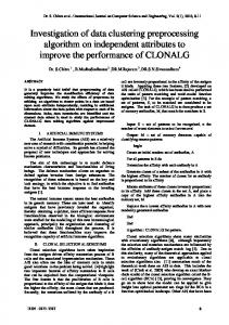
it completes, the slot is released so that other tasks can take it. Each slot can only have one task assigned at most at any time. There is a single central master node where Job Tracker runs. Job Tracker manages all slave/worker nodes and embraces a scheduler that assigns tasks to idle slots. Data locality is defined as how close compute and input data are, and it has different levels – node-level, rack-level, etc. In our work, we only focus on the node-level data locality which means compute and data are co-located on the same node. Data locality is one of the most important factors considered by schedulers in data parallel systems. Please note that here data locality means the data locality of input data. Map tasks may generate intermediate data, but they are stored locally (not uploaded to HDFS) so that data locality is naturally gained. We define goodness of data locality as the percent of map tasks that gain node-level data locality. In this paper, the default scheduling algorithm in Hadoop is denoted by dl-sched. In Hadoop, when a slave node sends a heartbeat message and says it has available map slots, the master node first tries to find a map task whose input data are stored on that slave node. If such a task can be found, it is scheduled to the node and node-level data locality is gained. Otherwise, Hadoop tries to find a task that can achieve racklevel data locality – input data and task execution are on the same rack. If it still fails, a task is randomly picked and dispatched. So dl-sched favors data locality and does not consider other factors such as system load and fairness. B. Goodness of Data Locality Firstly, we develop a set of mathematical symbols to characterize HDFS/MapReduce which are shown in Table I. Data replicas are randomly placed across all nodes. And idle slots are randomly chosen from all slots. This assumption is reasonable for modestly utilized clusters that run lots of jobs with diverse workload from multiple users. In such a complicated system, it is difficult, if not impossible, to know which slots will be released and when. In addition, we assume that I is constant within a specific time frame and may vary across time frames. This assumption implies that new tasks come into the system at the same rate that running tasks complete. So the system is in a dynamic equilibrium state for small time frames. Time is divided into time frames each of which is associated with a corresponding I. Our goal is to study the relationship between the goodness of data locality and significant system factors. Obviously, it depends upon scheduling algorithms. Default Hadoop scheduling algorithm dl-sched is the target of our analysis here. To simplify mathematical deduction, we assume replication factor C and the number of slots per node S are both 1. Firstly we need to calculate p(k, T) (the probability that k out of T total tasks can achieve data locality). Each task can be scheduled to any of the N nodes, so the total number of cases is NT. Because both the data placement and idle slot distribution are random, we can fix the distribution of idle slots without affecting the correctness of analysis. We simply assume that the first IS slots among all slots are idle. To guarantee that k tasks have data locality, we first choose k idle slots from total IS idle slots to which

unscheduled tasks will be assigned, which gives CkIS cases 1 in Fig. 1). Then we divide all unscheduled (shown as step ○ tasks into two groups: g1 and g2. For group g1, the input data of all its tasks are located on the nodes that have idle slots. For group g2, the input data of all its tasks are located on the nodes that have no idle slots. The input data of the tasks in group g1 need to be stored on k idle nodes so that exact k tasks can achieve data locality (note if the input data of multiple tasks are stored on the same node with only one idle slot, only one task can be scheduled to the node and other tasks will not achieve data locality). Assume group g1 has i tasks, the number of ways to choose these tasks from total T tasks is CiT , and the number of ways to distribute their input data onto k nodes is S(i, k) (stirling numbers of the second 2 in Fig. 1). The number of tasks in kind) (shown as step ○ group g2 is T-i and each of them can choose among N-IS busy nodes to store input data, which gives (N-IS)T-i cases 3 in Fig. 1). Combining all above steps, we ((shown as step ○ deduce (2) to calculate p(k, T). Then the expectation E can be calculated using (3) and the goodness of data locality R can be calculated using (4). TABLE I. Symbols N S I T C IS p(k, T) goodness of data locality

DEFINITIONS

Description the number of nodes the number of map slots on each node the ratio of idle slots the number of tasks to be executed replication factor the number of idle map slots (N * S * I) the possibility that k out of T tasks can gain data locality the percent of map tasks that gain node-level data locality

0 ≤ k ≤ T 0 ≤ T ≤ IS

p ( k , T ) = CkIS ⋅



T i =k

E=

(1)

(CiT ⋅ S (i, k ) ⋅ k !⋅ ( N − IS )T −i ) / N T (2)



T k =0

(k ⋅ p (k , T ))

R = E /T

(3) (4)

So the goodness of data locality can be accurately calculated. For cases where C and S are larger than one, the mathematical deduction is much more complicated and we are working on it. In our experiments below we take the

Figure 1. The deduction sketch for given i and k

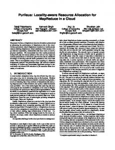
approach of simulation instead of accurate numerical calculation for two reasons: a) calculating (2) involves factorial and exponential operations requiring enormous computation if operands are large; b) we have not deduced closed-form formulas for the cases where C and S are not 1. C. Optimality of Scheduling In Terms of Data Locality Here the term optimality means the maximization of the goodness of data locality. Given a set of tasks to schedule and a set of idle slots, if a scheduling algorithm achieves the best data locality, we call it is optimal. We will show that scheduling multiple tasks all at once outperforms the taskby-task approach taken by dl-sched. 1) Non-optimality of dl-sched Fig. 2 demonstrates dlsched is not optimal. Fig. 2(a) shows an instantaneous state of a system. There are three tasks (T1, T2 and T3) to schedule, and three nodes (A, B and C) that have idle map slots. Each data block has multiple replicas and each node has three map slots among which those marked as black are not idle. If a data block B is marked with the same color and pattern as a task T, it means B is the input data of T. Only the nodes that have idle slots are shown. From the graph, we can see the input data of task T1 are stored on nodes A, B, and C; the input data of task T2 are stored on nodes A and B; and the input data of task T3 are stored on node A. Fig. 2(b) shows an example of dl-sched scheduling. Node A has one idle map slot and it hosts the input data of task T1, so T1 is scheduled to A. Node B has one idle map slot and hosts the input data of task T2, so T2 is scheduled to B. Now the only node that has idle map slots is C and task T3 must be scheduled there. However, node C does not host the input data of task T3. To summarize, tasks T1 and T2 gain data locality while task T3 loses data locality. But, we can easily find another way to schedule the three tasks to make all of them achieve data locality, which is shown in Fig. 2(c). The reason that dl-sched and its variants (e.g. fair scheduling, delay scheduling) are not optimal is that tasks are scheduled one by one and each task is scheduled without considering its impact on other tasks. To achieve a global optimum, all unscheduled tasks and idle slots at hand must be considered at once to make global scheduling decisions. 2) Optimal scheduling We reformulate the problem into a formal definition using symbols defined in section III (B). The assignment of maps tasks to idle slots is defined as function φ. Given task i, φ(i) is the slot to which it is assigned. Function φ needs to be injective to guarantee that multiple tasks are not assigned to the same idle slot. We associate an assignment cost to each task-to-slot assignment. Low assignment cost means good data locality and high assignment cost means bad data locality. Cij represents the assignment cost to assign task i to slot j, and is defined in (5). If a task is scheduled to a node which stores its input data, its assignment cost is 0. Otherwise, the cost is 1. Basically the cost matrix C measures the data

Figure 2. An example showing Hadoop scheduling is not optimal.

locality of assigned tasks. So it is good for IO intensive jobs and needs to be enhanced for other types of jobs. Given φ, the total assignment cost is the summation of the assignment cost of all scheduled tasks, which is formulated in (6). The goal function is shown in (7), which tries to find a φ that minimizes the total assignment cost. As we showed, the function φ given by dl-sched is not optimal, and therefore not a solution to (7). 1 ≤ i ≤ T ; 1 ≤ j ≤ IS 0 if the input data of task i and slot j collocate Cij =  otherwise 1 Csum (φ ) =



T i =1

Ciφ (i )

g = min C sum (φ )

(5)

(6) (7)

We found that this problem can be converted to the wellknown Linear Sum Assignment Problem[18] (LSAP) briefly described below. The difference is that LSAP requires that the cost matrix be square. In our case, if T and IS are equal, matrix C is square and we can directly apply LSAP. Otherwise, LSAP cannot be directly applied and we figure out how to convert the problem to LSAP by manipulating matrix C. Linear Sum Assignment Problem: Given n items and n workers, the assignment of an item to a worker incurs a known cost. Each item is assigned to one worker and each worker only has one item assigned. Find the assignment that minimizes the sum of cost. If T is less than IS, we make up IS-T extra dummy tasks whose assignment cost is 1 no matter which slots they are scheduled to. Fig. 3(a) shows an example in which ti and sj represent tasks and idle slots respectively. The first T rows are from the original cost matrix. The last IS-T rows are for the dummy tasks we make up and filled with constant 1. Now we get a IS x IS square cost matrix and can apply LSAP algorithms to find an optimal solution. LASP algorithms will give us an optimal assignment for all IS tasks. Among them we just pick those that are not dummy tasks, and we get a specific φ (termed φ-lsap) for the original problem. Now let

us prove that φ-lsap is a solution to (7) by using contradiction. Proof: The assignment cost given by φ-lsap is Csum(φlsap) (see (6)). As a result, the total assignment cost given by LSAP algorithms for the expanded square matrix is Csum(φ-lsap) + (IS-T). The key point is that the total assignment cost of dummy tasks is IS-T no matter where they are assigned. Assume that φ-lsap is not a solution to (7), and another function φ-opt gives smaller assignment cost. It implies Csum(φ-opt) is less than Csum(φ-lsap). We use the same mechanism to create dummy tasks and extend the cost matrix. We extend function φ-opt to include those dummy tasks and arbitrarily map them to the remaining IS-T idle slots. So the total assignment cost for the expanded square matrix is Csum(φ-opt) + (IS-T). Because Csum(φ-opt) is less than Csum(φ-lsap), we can deduce that Csum(φ-opt) + (IST) is less than Csum(φ-lsap) + (IS-T). That means the solution given by LSAP algorithm is not optimal. This contradicts with the fact that LSAP algorithms give optimal solutions. Constant 1 has been used as the assignment cost for dummy tasks. It turns out that we can choose any constant without violating optimality. The reason is the total assignment cost of all dummy tasks is a constant as well so that all task assignments perform equally well for dummy tasks. So what matters is the assignment of the T real tasks. It can be proved formally with the same method as above. s1 … sIS-1 sIS s1 ... sIS sIS+1 ... sT 1 1 0 0 t1 t1 1 … 1 1 1 1 … … … … … t2 0 … 0 1 1 1 0 1 1 0 tT t3 1 … 1 1 1 1 1 1 1 tT+1 1 t4 1 … 1 1 1 1 1 1 1 1 … … 1 … 1 1 1 1 1 1 1 1 tIS tT 1 … 1 1 1 1 (a) T < IS

(b) T > IS

Figure 3. Expand cost matrix to make it square. For (a), last IS-T rows are for dummy tasks we make up and all filled with 1. For (b), last T-IS columns are for dummy slots we make up and filled with 1.

For the case where T is larger than IS, we can use the same technique developed above to add extra T-IS columns representing dummy slots and fill them with 1, and therefore convert the original cost matrix to a square matrix. Fig. 3(b) shows an example. Then we can apply LSAP algorithms. After that, because dummy slots do not exist in reality, we remove those tasks that are assigned to dummy slots from the task assignment given by LSAP algorithms and get the final task assignment. We can prove its optimality ditto. Again, any constant can be used to fill the columns of dummy slots. We integrate LSAP into our proposed optimal scheduling algorithm lsap-sched shown below. It naturally follows our prior discussion. Function co-locate(T, S) checks whether slot S and the input data of task T are collocated on the same node. Function expandToSquare(C, value) expands matrix C to the closest square matrix by adding extra rows or columns filled with value. Function lsap(C) uses an existing LSAP algorithm to calculate the optimal assignment for cost matrix C. Function filterDummy(R) removes assignments for dummy tasks or dummy slots and returns the valid optimal

task assignment. Algorithm skeleton of lsap-sched Input: instant system state Output: assignment of tasks to idle map slots Algorithm: TS  the set of unscheduled tasks ISS  the set of idle map slots C  empty |TS| x |ISS| matrix for i = 0; i < |TS|; ++i for j = 0; j < |ISS|; ++j if co-locate(TS[i], ISS[j]) C[i][j] = 0 else C[i][j] = 1 if C is not square: expandToSquare(C, 1) R = lsap(C) R = filterDummy(R) return R

Now we investigate when lsap-sched can be applied. Generally, the more idle slots and tasks there are, the more lsap-sched outperforms dl-sched. For the extreme case where there is only one idle slot, dl-sched and lsap-sched perform equally well. For lightly used Hadoop clusters, a large portion of slots are idle. At the start of a new job, the scheduler has multiple tasks to schedule and multiple idle slots at disposal so that lsap-sched performs much better. For heavily used clusters, only a small number of slots are idle and the superiority of lsap-sched is not fully demonstrated if new tasks are scheduled immediately. Instead, scheduling can be delayed by a small amount of time before lsap-sched is applied so that “enough” idle slots are gathered. Tradeoffs between data locality and scheduling latency need to be made. It is our future work to decide scheduling latency adaptively and dynamically. IV.

EXPERIMENT

A. How Optimal is Default Hadoop Scheduling We have shown the default Hadoop scheduling algorithm dl-sched is not optimal. However, we are not clear yet about how non-optimal it is. In this experiment, we ran simulations to measure how close dl-sched is to the optimum. The reasons why we run simulations rather than use closed-form formulas have been explained in section III. We consider the case where the number of tasks to schedule is no greater than the number of idle slots. In the simulated system, the number of nodes was 100; the number of slots per node was 1; the number of idle slots was 50 (half of all slots were idle); and replication factor was 5. We varied the number of tasks from 1 to 50 and calculated the improvement of our proposed lsap-sched over dl-shed. We ran each test 10000 times and calculated the mean. Results are shown in Fig. 4(a). It clearly shows that as the number of tasks is increased, lsap-sched increasingly improves data locality over dl-sched. The goodness of data locality is improved by 14% at most when the system has equal number of unscheduled tasks and idle slots. Secondly, we varied replication factor between 1 and 19. The basic setup was the same as above except that the number of tasks was fixed to 50. Fig. 4(b) shows the results. The curve has a clear trend. As replication factor increases

from small values, the improvement of lsap-sched scheduling is increased drastically. At some point, the best improvement is reached. As replication factor increases further, the improvement decreases gradually. Theoretically, if each node has 1 slot, dl-sched is optimal for the extreme cases where replication factor is 1 or equals the number of nodes N. For those cases, it performs as well as lsap-sched. When replication factor falls between 1 and N, lsap-sched performs better. And there is a replication factor that makes lsap-sched outperform dl-sched most. In Hadoop, default replication factor is 3 and obviously lsap-sched scheduling is more efficient. Lastly, we varied the number of nodes between 10 and 200 with step size 10. Meanwhile, the number of tasks was changed accordingly to make it equal the number of idle slots so that all idle slots would be utilized (note the ratio of idle slots was fixed). The result is shown in Fig. 4(c). We observe that the improvement oscillates. We conjecture that it is caused by the fact that our simulation only covers a portion of all possible data placements and idle slot distributions. When there are 100 nodes and 50 tasks, the input data of each task can be placed onto any of the 100 nodes and the number of all possible placements is 10050. That number does not even take into consideration how idle slots are distributed across all slots. So it is impossible to enumerate all possible cases and calculate result for each.

(a)Data locality impr. vs. Num. of tasks(b)Data locality impr. vs. Rep. factor

(c) Data locality impr. vs. Num. of nodes Figure 4. Data locality improvement of lsap-sched over dl-sched

B. Impact of Various Factors on Data Locality In this set of tests, we evaluate how different factors impact the goodness of data locality. The investigated factors include the number of tasks, the number of map slots per node, replication factor, the number of nodes and the ratio of idle map slots. The configuration is shown in table II. For each test, we varied one factor while fixing all others. All results are shown in Fig. 5. Fig. 5(a) shows how the goodness of data locality changes with the number of tasks. We observe that the goodness of data locality decreases as the number of tasks is increased initially. When the number of tasks becomes 27 (128), data locality is the worst. As the number of tasks is

(a) Vary the number of tasks

(e) Vary the number of nodes

(b) Vary the number of slots per node

(f) Redraw (a) and (e) using different x-axes

(c) Vary replication factor

(g) Real trace copied from [4]

(d) Vary the ratio of idle slots

(h) Sim. result with similar config

Figure 5. Impact of various factors on the goodness of data locality and Comparison of real trace and simulation result

increased further beyond 27, the ratio of data locality increases quickly. The degree of increment is decreased as there are more and more tasks. TABLE II.

SYSTEM CONFIGURATION

Parameter

Default value

Range (used when a factor is tested)

Env. in Delay Sched. Paper

num. of nodes

1000

[300, 5000]; step 100

1500

slots per node

2

[1, 32]; step 1 0

1

13

2 4

num. of tasks

300

(2 , 2 , …, 2 )

(2 , …, 213)

ratio of idle slots

0.1

[0.01, 1]; step 0.02

0.01

replication factor

3

[1, 20]; step 1

3

Increasing the number of slots per node results in more idle slots, as the ratio of idle slots is fixed. Its impact on data locality is shown in Fig. 5(b). The data locality improves drastically as the number of slots per node increases initially. 5, 8 and 10 slots per node give the goodness of data locality 50%, 80% and 90% respectively. Considering the reality that modern server nodes have multiple cores and multi processors, it is reasonable to allow 5-10 tasks to run concurrently on each node. So to specify more slots per node improves not only the resource utilization ratio but also the data locality. Prior research investigated the impact of concurrently running tasks on resource usage, but has not explored its impact on data locality. Our result quantifies the relationship and serves as guidance for users to tune the system. The impact of replication factor is shown in Fig. 5(c). As we expect, replication factor has positive impact, which means the increase of replication factor gives better data locality. However, the relationship between replication factor and data locality is not linear. The degree of improvement decreases with increasing replication factor. Obviously, more storage space is required as replication factor is increased and that relationship is linear. Fig. 5(c)

can help system administrators choose the best replication factor that balances storage usage and data locality, because it tells how much data locality is lost/gained when replication factor is decreased/increased. As replication factor gets larger and larger, the benefit becomes more and more marginal. Based on how scarce storage space is, the sweet spot of replication factor can be carefully chosen according to Fig. 5(c) to achieve the best possible data locality, compared with the case where replication factor is arbitrarily chosen. Fig. 5(d) shows the impact of varying the ratio of idle slots. When the ratio of idle slots is around 40% and therefore the utilization ratio is 60%, the goodness of data locality is over 90%. This means the utilization ratio of all slots need not be very low to get a reasonably good data locality, which is a little counter-intuitive. Even if most of the slots are busy, the goodness of data locality can still reach around 30% given that many tasks are to be scheduled, because the scheduler can choose the tasks that can achieve the best data locality among all unscheduled tasks at hand. A general intuition is that as more nodes are added to a system, the performance usually should be improved. However, the degree of performance improvement is not necessarily linear with the number of nodes. In this test, we increased the number of nodes from 300 to 5000 and the results are shown in Fig. 5(e). Surprisingly, the goodness of data locality drops as we add more nodes initially. When there are around 1500 nodes, the goodness of data locality becomes the lowest. Beyond 1500, the goodness of data locality is positively related to the number of nodes. To figure out why 1500 is the stationary point, we calculated the ratio of the number of idle slots to the number of tasks, which is used as the x-axis in Fig. 5(f). Data locality is the worst when there is equal number of idle slots and tasks. We also redraw Fig. 5(a) using the same transformation and present the result in Fig. 5(f). The two curves in Fig. 5(f) have the similar shapes. From these two plots, we can see

that data locality deteriorates sharply when there are less idle slots than tasks and the ratio between them increases. Under these circumstances, tasks need to be scheduled in multiple waves for all of them to run. For each wave, the scheduler can cherry-pick from remaining tasks those that can achieve the best data locality. As the number of idle slots gets close to the number of tasks, the freedom of cherry-picking is decreased because in each wave more tasks need to be scheduled. The freedom is totally lost when the numbers of tasks and idle slots are equal because all tasks need to be scheduled in one wave. When there are more idle slots than tasks, the scheduler can cherry-pick the slots that will give the best data locality. To summarize, when there are less/more idle slots than tasks, the scheduler can cherry-pick tasks/idle slots among all possible assignments to obtain the best locality. The degree of cherry-picking freedom increases as the difference between the numbers of idle slots and tasks gets larger. Another observation is that the curve is not symmetric with respect to the vertical line ratio=1. The loss of data locality when the ratio grows towards 1 is much faster than the regaining of data locality when the ratio grows beyond 1. When the number of tasks is 40 times that of idle slots, the goodness of data locality is above 90%; while it is only around 50% when the number of idle slots is 200 times that of tasks. Tests in Fig. 5(b), (d) and (e) all result in the change of idle slots with the number of tasks fixed, but they have different curves. The critical difference is that in Fig. 5(e) the number of nodes is changed while in Fig. 5(b) and (d) the number of nodes is constant. The difference of those curves originates from the fact that tasks are scheduled to slots while input data are distributed to nodes. For Fig. 5(b) and (d), the distribution of data is constant and task scheduling varies according to the change of the number of idle slots. Having more nodes means the input data of a set of tasks are more spread out, which has a negative impact on data locality. For Fig. 5(e), both data distribution and idle slot distribution vary. Increasing the number of slots per node is not equivalent to adding more nodes in terms of data locality. To verify how close our simulation is to the real system in terms of accuracy, we compared a real trace and our simulation result. In [12], the authors analyzed the trace data collected from Facebook production Hadoop clusters. They found that the system is more than 95% full 21% of the time and 27.1 slots are released per second. The total number of slots is 3100, so the ratio of idle slots is 27.1 / 3100 ≈1%. We could not find the number of slots per node in the paper. So we assumed the Facebook cluster uses the default Hadoop setting: 2. Then we can deduce that there are 3100/2 ≈ 1500 nodes in the system. Replication factor is not explicitly mentioned in the paper for the trace and we assumed the default Hadoop setting 3 is used. The cluster configuration is summarized in the last column of table II. The authors measured the relationship between percent of local map tasks and job size (number of map tasks). We duplicate their plot in Fig. 5(g), in which both node locality and rack locality are shown. We ran simulation tests with the same configuration and show results in Fig. 5(h). By comparing the two plots, we observe that our simulation gives reasonably good

results. Firstly, the curves are similar and both have an “S” shape. Secondly the concrete y values are also close. So the assumptions we made are valid for real clusters. As we said, although the ratio of idle slots in real systems is not constant across time, we can divide the whole time span into shorter periods (e.g. peak hours, off-peak hours) for each of which the ratio of idle slots is approximately constant and our simulation can be conducted. C. Impact of Data Locality in Single-Cluster Environments In this test, we evaluate how important data locality is in single-cluster Hadoop systems. In other words, we want to know to what extent performance will degrade due to the deterioration in data locality. We wrote a random scheduler rand-sched which by default randomly assigns tasks to idle slots so that data locality greatly worsens. In addition, users can specify a parameter called randomness which tells randsched how random the scheduling should be. If its value is 100%, the scheduling will be thoroughly random; if its value is 0%, rand-sched degenerates to dl-sched. Other values give a mixture of random and default scheduling. We compared the cases where rand-sched with randomness 0.3, 0.5, 0.7 and 1 and dl-sched were applied. An IO intensive application input-sink, which mainly reads data from HDFS, was written and used in the tests. We calculated the slowdown of rand-sched relative to dl-sched and show it in Fig. 6. The horizontal line y=0 is the baseline which implies the performance is as good as dl-sched. We observe that rand-sched with randomness 1 gives the worst performance and the slowdown is positively related to randomness. D. Impact of Data Locality in Cross-Cluster Environments 1) With high-speed interconnection among clusters: In this test, we evaluate how Hadoop performs in cross-cluster environments. We categorize deployments into three classes: single-cluster, cross-cluster and HPC-style. For cross-cluster deployments, HDFS and MapReduce share the same set of nodes that are distributed across multiple physical clusters. For HPC-style deployments, HDFS uses nodes in one cluster and MapReduce uses nodes in another cluster so that storage and compute are totally separated. We used clusters in FutureGrid that are equipped with highspeed inter-cluster network. Each node has 8 cores and gigabit Ethernet. Single-cluster deployments used 10 nodes in cluster India; cross-cluster deployments used 5 nodes in India and 5 nodes in Hotel; HPC-style deployments used 10 nodes in India for MapReduce and 10 nodes in Hotel for HDFS. Again, input-sink was used as test application, and results are shown in Fig. 7(a). The plot matches our intuitive expectation. HPC-style deployment thoroughly loses data locality and performs the worst. dl-sched in single-cluster deployments performs the best. However, dlsched in cross-cluster deployments performs better than rand-sched in single-cluster deployments. The reason is those clusters only see light use and the interconnection between clusters is fast enough to match the speed of local network to fulfill read/write requests.

cluster and HPC-style setup, have been discussed and real Hadoop experiments were conducted. It shows data locality is important to single-cluster deployments. Also it shows the inability of Hadoop to cope with significant network heterogeneity and inter-cluster connection is critical to performance. ACKNOWLEDGMENT Figure 6. Single-cluster performance

2) With drastically heterogeneous network We set up a unified Hadoop cluster across multiple physical clusters by building a virtual network overlay with ViNe[19]. To know to what extent performance is impacted by the throughput of inter-cluster links, ViNe provided low throughput: only 110Mbps. We compared rand-sched with dl-sched and show results in Fig. 7(b). The loss of data locality slows down the execution by thousands of times. The results also apply to the case where the inter-cluster network is fast but heavily oversubscribed so that on average each application can only get a fairly small share. This demonstrates that Hadoop is not optimized for fairly heterogeneous networks (e.g. WideArea Network) so that Hadoop deployments over geographically distributed clusters with oversubscribed interconnection should be carefully investigated.

This material is based upon work supported in part by the National Science Foundation under Grant No. 0910812. REFERENCES [1]

[2]

[3] [4] [5] [6]

[7]

[8]

[9]

(a) with high-speed cross-cluster net (b) with drastically heterogeneous net

[10]

Figure 7. Cross-cluster Hadoop performance [11]

V.

CONCLUSION

The overall goal of this paper is to investigate data locality in depth for data parallel systems, among which GFS/ MapReduce is representative and therefore our main research target. We have mathematically modeled the system and deduced the relationship between system factors and data locality. Simulations were conducted to quantify the relationship and some insightful conclusions have been drawn which can help to tune Hadoop effectively. In addition, non-optimality of default Hadoop scheduling has been discussed and an optimal scheduling algorithm based on LSAP has been proposed to give the best data locality. We ran intensive experiments to measure how our proposed algorithm outperforms default scheduling and demonstrate its performance superiority. Above research uses data locality as a performance metric and the target of optimization. Besides that, we investigated how data locality impacts the user-perceived metric of system performance: job execution time. Three scenarios – single-cluster, cross-

[12]

[13]

[14] [15] [16]

[17] [18] [19]

C.S. Chang. “Needs for Extreme Scale DM, Analysis and Visualization in Fusion Particle Code XGC,” CPES at Exascale data management, Analysis, and Vis., Feb. 22-23, 2011, Houston, TX. Scientific Grand Challenges: Fusion Energy Sciences and the Role of Computing at the Extreme Scale. U. S. Department of Energy, March 18-20, 2009. Washington DC J. Chen and J. Bell, “Combustion Exascale Co-Design Center,” 6th IESP Workshop, San Francisco, CA, April 6-7, 2011 S. Ghemawat, H. Gobioff, and S. Leung, “The Google file system,” In Proc. of SOSP 2003. New York, NY, USA, 29-43. K. Shvachko, H. Kuang, S. Radia, and R. Chansler, “The Hadoop Distributed File System,” IEEE MSST 2010 M. Isard, M. Budiu, Y. Yu, A. Birrell, and D. Fetterly, “Dryad: distributed data-parallel programs from sequential building blocks,” In Proc. of EuroSys 2007. ACM, New York, NY, USA, 59-72. J. Ekanayake, T. Gunarathne, J. Qiu, G. Fox, et. al., “Applicability of DryadLINQ to Scientific Applications,” January 30, 2010, Tech report in Community Grids Laboratory, Indiana University. Y. Gu and R. Grossman, “Sector and Sphere: The Design and Implementation of a High Performance Data Cloud,” Crossing boundaries: computational science, e-Science and global eInfrastructure, I. Trans. R. Soc. A, 2009. vol. 367, p. 2429-2445. K. Ranganathan and I. Foster, “Decoupling computation and data scheduling in distributed data-intensive applications,” In Proc. of HPDC 2002, p. 352- 358, 2002 F. Chung, R. Graham, R. Bhagwan, S. Savage, and G. M. Voelker, “Maximizing data locality in distributed systems,” J. Comput. Syst. Sci. 72, 8 (December 2006), 1309-1316. H. H. Mohamed and D. H. J. Epema, “An evaluation of the close-tofiles processor and data co-allocation policy in multiclusters,” In Proc. of Cluster 2004, p. 287- 298, 20-23 Sept. 2004 M. Zaharia, D. Borthakur, J. Sarma, K. Elmeleegy, S. Shenker, and I. Stoica, “Delay scheduling: a simple technique for achieving locality and fairness in cluster scheduling,” In Proc. of EuroSys 2010, New York, NY, USA, 265-278. B. Palanisamy, A. Singh, L. Liu and B. Jain, “Purlieus: Localityaware Resource Allocation for MapReduce in a Cloud,” In Proc. of SC 2011 Z. Guo, M. Pierce, G. Fox and M. Zhou, “Automatic Task Reorganization in MapReduce” CLUSTER2011, Sep. 2011, Austin, TX. Y. Luo, Z. Guo, Y. Sun, et. al. “A Hierarchical Framework for CrossDomain MapReduce Execution,” HPDC workshop ECMLS 2011 M. Zaharia, A. Konwinski, A. D. Joseph, R. Katz, and I. Stoica, “Improving MapReduce performance in heterogeneous environments,” In Proc. of OSDI 2008, Berkeley, CA, USA https://issues.apache.org/jira/browse/HADOOP-2141 http://www.assignmentproblems.com/doc/LSAPIntroduction.pdf M. Tsugawa and J. Fortes, “A Virtual Network (ViNe) Architecture for Grid Computing,” IPDPS 2006, p. 10, April 2006