Investigation of Neural Networks for Function ... - Semantic Scholar

Available online at www.sciencedirect.com

Procedia Computer Science 17 (2013) 586 – 594

Information Technology and Quantitative Management (ITQM2013)

Investigation of Neural Networks for Function Approximation Sibo Yang, T.O. Ting*, K.L. Man and Sheng-Uei Guan Xian Jiaotong-Liverpool University, Suzhou, China

Abstract In this work, some ubiquitous neural networks are applied to model the landscape of a known problem function approximation. The performance of the various neural networks is analyzed and validated via some well-known benchmark problems as target functions, such as Sphere, Rastrigin, and Griewank functions. The experimental results show that among the three neural networks tested, Radial Basis Function (RBF) neural network is superior in terms of speed and accuracy for function approximation in comparison with Back Propagation (BP) and Generalized Regression Neural Network (GRNN). © 2013 2013 The byby Elsevier B.V.B.V. © The Authors. Authors.Published Published Elsevier Selection and/or peer-review under responsibility of the the organizers Conference on Computational Selection and peer-review under responsibility of organizersofofthe the2013 2013International International Conference on Information Science Technology and Quantitative Management Keywords: benchmark function; function approximation; neural network.

1. Introduction A neuron is a model based on the nerve cell of biological nervous system and is the minimum unit that processes biological information [1, 2]. It consists of cell body, dendrite and axon. The cell body is the source of energy; dendrite is the structure to receive the message of other neurons and axon is the transmission part to send and output neural impulse. A large number of neurons form the entire nervous system, which is multi-cell, nonlinear, and dynamitic system. Artificial Neural Network (ANN) is a tool to simulate the biological nervous system to process the information [1, 2]. Benefiting from physiological results on the brain, neural network simulates the relevant nonlinear and dynamitic system to achieve the special features. Besides, the network has the adaptive, organized and learning abilities [2-6]. The artificial neuron is the basis of ANN. As shown in Figure 1, it can be treated as the integration of three parts, that are a group of inputs and weights, a transfer function such as an adder and an activation function with a threshold [2, 7-9]. The sign of the weight represents the state of the relevant component. Usually, the positive sign is the symbol of activated state and the negative sign denotes nonactivated state. The normal range of the output of an artificial neuron is within the interval of (-1, +1) or (0, 1) [2,

*

Corresponding author. Tel.: +86-512-88161416; fax: +86-512-88161899. E-mail address: [email protected]

1877-0509 © 2013 The Authors. Published by Elsevier B.V. Selection and peer-review under responsibility of the organizers of the 2013 International Conference on Information Technology and Quantitative Management doi:10.1016/j.procs.2013.05.076

587

Sibo Yang et al. / Procedia Computer Science 17 (2013) 586 – 594

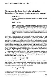
10]. ANNs are grouped into two categories based on the different types of connections between artificial neurons: the hierarchical neural network. This is shown as (a) and (b) of Figure 2. ANNs contain input, hidden and output layers. From the outside, hierarchical network is the feed-forward neural network. In this case, the connected neural network may be changing frequently and consequently, which forms an output mode and at times it may fall into a periodicity or a chaos state [1, 2]. weights inputs

x1

w1j Activation function

x2

w2j

x3

w3j

...

...

xn

wnj

Net input netj

oj activation

Transfer function

j

threshold

Fig 1. The components of artificial neuron

INPUT LAYER

INPUT LAYER

HIDDEN LAYER

HIDDEN LAYER

X1

H1 X2

OUTPUT LAYER

X1

OUTPUT LAYER

H1

Z1

Y1

X2

Z1

Y1

Z2

Y2

X3

Z2

Y2

H2 X3 H3

X4

H2

X4

(b) Connected neural network

(a) Hierarchical neural network Fig 2. Types of neural network

When the network is processing information, the network is transforming constantly. The network is also nonconvex, which may have more than one extreme value [2, 11]. To solve a real-world problem, an appropriate configuration of model or function is necessary. The number of neurons and effective multilayer perceptron are the common key topics. MATLAB has Neural Network Toolbox, the Neural Network Fitting Tool and the corresponding GUI. It provides the network design and training sub programs [1, 2, 5, 8, 12]. In this paper, we apply three types of well-known neural networks namely Back Propagation (BP), Radial Basis Function (RDF) and Generalized Regression (GN) to model or approximate the landscape of known functions. The results are displayed in the form of 3D graphs and total error calculated from each neural network is presented numerically.

588

Sibo Yang et al. / Procedia Computer Science 17 (2013) 586 – 594

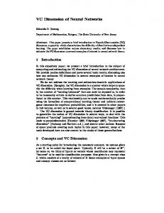
2. Methodology Basically, there are seven steps involved in the context of function approximation. The first step is the data collection, given in the form of matrix input. Then, the relevant network will be created and configured. After the configuration, the weights and biases are initialized. Further, training and validation are carried out by utilizing the data generated from the known benchmark function. After training and validation, the neural network is complete and ready for further testing and justification [8]. In this work, three different neural networks are applied for function approximation. These are Back Propagation (BP), Radial Basis Network (RDF) and Generalized Regression Neural Network (GRNN). 2.1. Back Propagation Neural Network The Back Propagation (BP) neural network is a kind of multi-layer feed forward network. The transfer function is S-function [4, 9]. Due to the adjustment of weights under the BP learning, the network is called the BP neural network. The output of the BP neuron can be expressed: (1) whereby f is the transfer function, representing the relationship between the input and the output. The transfer function is usually denoted by log-sigmoid, tan-sigmoid or purely linear function. This is illustrated in Figure 3. The learning process has two parts: the first part is learning through the setting of the structure and the previous weight and threshold; the second part is adjusting the weight and threshold through the gradient of last layer [4, 6, 9]. The BP algorithm is one of -model algorithm and is a kind of supervised learning. For instance, Figure 4 demonstrates a typical two-layer BP neural network.

n

a = logsig(n)

n

n

a = tansig(n)

a = purelin(n)

Fig. 3. The transfer function of the BP neuron

There are many improved versions of BP algorithm. For instance, steepest descent back propagation (SDBP), momentum back propagation (MOBP), variable learning rate back propagation (VLBP), resilient back propagation (RPROP) and conjugate gradient back propagation (CGBP), Quasi-Newton algorithms and Levenberg-Marquardt (LM) algorithm [13].

589

Sibo Yang et al. / Procedia Computer Science 17 (2013) 586 – 594

Input p1 2×1

Hidden Layer

IW1,1 4×2

Output Layer a1

n1

4×1

LW2,1 3×4

4×1

1 2

n2

3×1

3×1

b1 4×1

a3 -y

1 4

a1 = tansig(IW1,1p1 +b1)

b2 3×1

3

a2 = purelin(LW2,1a1 +b2)

Fig. 4. The typical two-layer BP network

In this paper, the improvement based on LM algorithm is chosen. The basis of this method is given by: (2) A(k) is Hessian matrix (second order derivate) when the error performance function is under the weight and threshold [6]. The LM algorithm is used to avoid the calculation of Hessian matrix. When the error performance has the form square and error (typical error function for training in the feed forward network), the Hessian matrix can be written as (3) (4) whereby H is a Jacobian matrix that contains the error function. The e is the error vector of the network. Therefore, based on the approximation of the Hessian matrix, the method is changed to: (5) 2.2. Radial Basis Function (RBF) RBF network is a three-layer feed forward network. The input layer comprises the nodes of input signal; the number of hidden unit is determined by the specific problem and the transfer function of RBF is an attenuation, central-radial symmetry, non-negative and non-linear function [3]. The output layer is the response of the input model. The relationship between input and hidden layer is non-linear and the relationship between the hidden layer and output layer is linear [3, 14]. The basic idea of RBF network is the basis which uses RBF as hidden unit consisting of hidden space. It is able to map the input vector to the hidden space directly. When the central point of RBF is confirmed, its mapping relationship is determined. Moreover, the mapping from hidden space to output space is linear. In other words, the output of network is the summation of linear weight in the hidden unit. The weight here is adjustable parameter of network. Generally, the network mapping from input to output is nonlinear [3, 7]. However, the network output for adjustable parameter is linear. In this case, the network weight is worked out directly according to the linear function. This greatly accelerates the study rate and avoids the problem of part minuteness [7, 14]. RBF neuron network is also known as radial basis function neural network. It takes a Gaussian function to realize the mapping from the output space into the hidden space, and Gaussian can be represented by:

590

Sibo Yang et al. / Procedia Computer Science 17 (2013) 586 – 594

whereby is the center point of the jth basis function; is called stretch constant. We use stretch constant to determine each radial basis neuron and its output vector, namely the area width corresponding to the distance from x to . As noted, the weight of radial basis neuron is processing gradually. Usually, the weight of the hidden space of each group is larger than the output vector. In fact, the network is working partially; this means that for each group input, there is only one neuron of hidden space that is activated in network, the value of other neuron output can be ignored. Therefore, the radial basis function network is a partial working network. The output expression is: (6) whereby radbas() is radial basis function, generally as Gaussian function: (7) It has good smoothness, mirror symmetry and a simple form: (8) Radial basis function network model is also a back propagation neuron network, it has two network layers: hidden space as radial space; linear space as output. Input

Radial Basis Layer

Linear Layer

IW1,1 p

||dist||

R×1 * ·

1 R

a1

S1×1

S1×1

n1

1

b

S1×1

S1

ai1 = radbas(||IW1,1-p1 || bi1)

b2

S2×1

n2

S2×S1

S1×1

1

a3 =y

LW2,1

S2×1

S2×1

S2

a2 = purelin(LW2,1a1 +b2)

Fig. 5. The structure of radial basis function

The learning variables of RBF are the center and variance of the basis function and the weight of hidden layer and output layer. The normal learning method is the self-organized center selection method. The characteristic is that the center and weight are independently determined. It has two steps: the first one is self-organized step. It learns the center and variance of the function in the hidden layer; the second one is supervised learning to learn the weight of output layer [3, 7, 14]. 2.3. Generalized Regression Neural Network (GRNN) GRNN network structure is similar to the radial basis function network and it just has tiny difference in the second layer. This is illustrated in Figure 6. The number of the vector pairs of neuron and output expectations

591

Sibo Yang et al. / Procedia Computer Science 17 (2013) 586 – 594

sample are equal. The weight of first layer is p , threshold

is the column vector of

. The principle to find

spread is to adjust the distance between the input vector and neuron weight vector to 0.5. The network input of neuron in first layer is the product of weight input and corresponding threshold, and then according to the neuron function radbas to calculate the network output of first layer neuron network. As such, the weight input representing the distance between the input vector and weight vector; it can be obtained by calculating the value of dist [7]. The number of neurons of GRNN in the second layer is the same as the input expectation sample vector pairs [7]. Input Q×R

p

IW1,1 Q×Q ||dist||

* ·

R

LW2,1

a2 -y

Q×1

R×1

1

Special Linear Layer

Radial Basis Layer

n1

at

Q×1

Q×1

nprod

n2

Q×1

Q×1

bt Q×1

Q

ai1 = radbas(||IW1,1-p1 || bi1)

Q

a2 = purelin(n2)

Fig. 6. The structure of generalized regression neural network

Dispersion constant spread has a great relationship between the output figure of network. When the spread is wide, the covered input region is large. On the contrary, if the spread is narrow, the curve of radial basis function is relatively steep, and the neuron output relative to the weight approach the input vector is much bigger than others, network output is closer to the expectation [7]. In general, the bigger the spread, the smaller the steep of its radial basis function curve. To sum up, the network output is the total of the average weight values of the input vector that is closed to the sample expectations. 3. Experimental Results In this section, three benchmark functions are utilized for the approximation. The mathematical representations of Sphere, Rastrigin and Griewank functions are given as (9), (10) and (11) respectively: (9) (10) (11) The relevant settings concerning these problems are given in Table 1. The resolution values in the last column of Table 1 are values smaller than the shortest distance between local optima present. As such, there exists no loss of information between any two points. For instance, for the case of Sphere, the resolution is set to high value as this is appropriate to represent the nature of this smooth curve. This value is determined through graphical analysis of high resolutions 3D graph. This is to ensure the generation of appropriate and adequate data for effective training. The resolutions of Rastrigin and Griewank are more challenging as these are both multimodal problems. By meticulous analysis, we come to the conclusion that setting their values to 0.2 and 0.4 is adequate

592

Sibo Yang et al. / Procedia Computer Science 17 (2013) 586 – 594

for the function approximation process. Table 1. The variables of Benchmark function Function

Dimension

Range

Resolution

Sphere

2

10

Rastrigin

2

0.2

Griewank

2

0.4

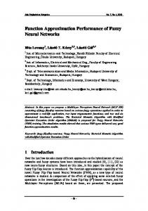
Three types of neural network, elaborated in Section II is applied to learn the landscape of the functions in Table 1. Firstly, we generate the input and output data using the mathematical formulas of these functions. Then, a neural network is chosen for the approximation. The data generated is then applied for training, testing and validation. The results are presented graphically in the following section. 4. Results and Discussions Results of all three neural networks are presented here. The mean squared error for all three functions are summarized in Table 2. In the case of sphere function, the BP neural network is the best approximated as it records the lowest MSE of 0.1793. However, for the case of Rastrigin function, BP NN fails to learn the complicated structure of this function. The graphical output as illustrated in Figure 7(b) shows truncated landscape of the function. For this function, RBF is the best approximator, recording an MSE of 0.1987. Table 2. The Result of Sphere Function Function Neural Network Setting MSE

Sphere BP Epoch: 1000 Goal: 0 0.1793

(a) Target function

RBF Goal: 0.2 Spread: 10 23.59

Rastrigin GRNN Spread: 10 7.89×104

BP

RBF

Epoch: 1000 Goal: 0.2 Goal: 0 Spread: 0.2 ----

0.1987

Griewangk GRNN Spread: 0.2 0.5691

(b) Output value from BP

BP

RBF

GRNN

Epoch: 1000 Goal: 0.2 Spread: 0.4 Goal: 0 Spread: 0.4 ----

0.5601

0.5600

Sibo Yang et al. / Procedia Computer Science 17 (2013) 586 – 594

(c) Output value from RBF

(d) Output value from GRNN Fig. 7. The outputs from the networks for problem approximation

For the third case, Griewank function, again BP fails to obtain satisfactory result. The best approximator here is GRNN, recording MSE of 0.56, slightly smaller in comparison to RBF. The graphical outputs from both neural networks portrays smooth surface landscape which is almost identical to the target function. Based on the results above, BP method is good to approximate Sphere function and the performance deteriorates greatly when applied to Rastrigin and Griewank functions. In both of these cases, there exists a phenomenon that the training data seems not efficient. There are two reasons that caused the poor results. The first is the adjustment of weight and the second is the minimum value in some local parts. A larger changing weight can cause the sum of majority or even all the neurons to increase greatly, thereby keeping the input of activated function in the saturation parts of transfer function and suspending the process of adjusting weight. A local minimum value can be derived from the BP method, but this value cannot locate the global minimum as BP method is based on the decreasing gradient. The gradually decreasing gradient follows the slope of error function in the training process. Moreover, in order to acquire a minimum error, the training time is also longer. A progress of 100000 epochs requires approximate 1 hour in MATLAB. 5. Conclusions RBF and GRNN methods are efficient to approximate Sphere, Rastrigin and Griewank functions. From the approximation perspective, a neural network can be regarded as the approximator of unknown model or problem landscape. Therefore, any function can be represented by the weighted sum of a group of basic functions. In RBF and GRNN, this is possible via the transfer function of neuron in hidden layers. Although the output mapping from the input is non-linear, the output is linear to the weight, which is a tunable parameter. During the process of function approximation using RBF and GRNN, the dispersion constant should be the same as the resolution of functions, which is the distance between the input vectors. Large and small dispersion constant will lead to fewer and more neurons. Fewer neurons will cause the overlap of the inputs and outputs. Subsequently, the neural network is unable to provide different responses and the approximation will be in non-fit condition. On the contrary, more neurons will result in the over-fit phenomenon in the approximation. From the results, RBF and GRNN are better approaches when it comes to function approximation. Besides, the RBF and GRNN avoid local minimum as compared to BP method. In future work, the neural network will be applied to a wider range of benchmark functions to validate its efficiency.

593

594

Sibo Yang et al. / Procedia Computer Science 17 (2013) 586 – 594

ACKNOWLEDGEMENTS The authors would like to acknowledge the SURF sponsorship granted by to support this research work.

-Liverpool University

REFERENCES [1] [2] [3] [4] [5] [6] [7] [8] [9] [10] [11] [12] [13] [14]

Z. Chonglin, Y. Lijuan, and W. Weibing, "Study on fitness data processing based on neural network information processing," in International Conference on Systems and Informatics (ICSAI), 2012, 2012, pp. 295-298. Z. Ying, G. Jun, and Y. Xuezhi, "A survey of neural network ensembles," in International Conference on Neural Networks and Brain, 2005. ICNN&B '05., 2005, pp. 438-442. H. Husain, M. Khalid, and R. Yusof, "Nonlinear function approximation using radial basis function neural networks," in Student Conference on Research and Development, 2002, pp. 326-329. L. Marquez and T. Hill, "Function approximation using backpropagation and general regression neural networks," in Proceeding of the Twenty-Sixth Hawaii International Conference on System Sciences, 1993, vol. 4, pp. 607-615. T. Varshney and S. Sheel, "Approximation of 2D function using simplest neural networks; A comparative study and development of GUI system," in 2010 International Conference on Power, Control and Embedded Systems (ICPCES), 2010, pp. 1-4. G. Hongliang, "The probability characteristic of function approximation based on artificial neural network," in 2010 International Conference on Computer Application and System Modeling (ICCASM), 2010, pp. V1-66-V1-71. F. Heimes and B. van Heuveln, "The normalized radial basis function neural network," in IEEE International Conference on Systems, Man, and Cybernetics, 1998, vol. 2, pp. 1609-1614. Jayadeva, A. K. Deb, and S. Chandra, "Algorithm for building a neural network for function approximation," IEE Proceedings -Circuits, Devices and Systems, vol. 149, pp. 301-307, 2002. R. Setiono and A. Gaweda, "Neural network pruning for function approximation," in International Joint Conference on Neural Networks, 2000. IJCNN 2000, Proceedings of the IEEE-INNS-ENNS, 2000, vol. 6, pp. 443-448. S. Ferrari and R. F. Stengel, "Smooth function approximation using neural networks," IEEE Transactions on Neural Networks, vol. 16, pp. 24-38, 2005. Y. Shiow-Shung and T. Ching-Shiow, "An orthogonal neural network for function approximation," IEEE Transactions on Systems, Man, and Cybernetics, Part B: Cybernetics, vol. 26, pp. 779-785, 1996. N. Kouda and N. Matsui, "On the function approximation in Restricted Coulomb Energy neural network with Gaussian Radial Basis Function," in World Automation Congress (WAC), 2010, 2010, pp. 1-5. G. Yue-Seng and T. Eng-Chong, "An integrated approach to improving back-propagation neural networks," in TENCON '94. Proceedings of 1994 IEEE Region 10's Ninth Annual International Conference. Theme: Frontiers of Computer Technology, 1994, vol.2, pp. 801-804. T. Jea-Rong, C. Pau-Choo, and I. C. Chein, "A sigmoidal radial basis function neural network for function approximation," in 1996 IEEE International Conference on Neural Networks, vol. 1, pp. 496-501.