learning in the competitive artificial neural networks and present the Matlab
environment for their implementation. INTRODUCTION. Creating networks, which
...
KNOWLEDGE EXTRACTION WITH COMPETITIVE NEURAL NETWORKS IN MATLAB ENVIRONMENT
Luminita Giurgiu, Assistent Professor, Land Forces Academy “Nicolae Balcescu”, Sibiu, Revolutiei 3-5, tel. 0040269432990/1413, fax 0040269215554, email:
[email protected]
Abstract. The desire to develop computer systems that can learn by themselves and improve decision-making is an ongoing goal of information technology. The field of artificial neural networks is a powerful emerging technology that can be used to efficiently process information to achieve greater knowledge and improved decision making. Neural networks self-adapt to learn from information, providing powerful models representing knowledge about a specific problem. In this paper we discuss the process of unsupervised learning in the competitive artificial neural networks and present the Matlab environment for their implementation. INTRODUCTION Creating networks, which find patterns in data sets without supervision, implies a process of unsupervised learning. Behind unsupervised learning is competition. Self-organizing networks can learn to detect regularities and correlations in their input and adapt their future responses to that input accordingly. Such networks are competitive networks and Self-organizing maps. Competitive networks are two layers and fully connected. The weights on the connections are normally set to random positive values in the range 0 to 1. As usual, inputs are applied to the input layer, and the outputs from the output layer nodes are considered. Now, there are no known corresponding correct outputs, as was the case in the supervised learning situation. In this case, have a contest. A node with its weight vector closest to the vector of inputs is declared the winner, and only its weights are adjusted by some training algorithm. This process is then repeated for each input vector, over and over, for a large number of cycles. Different inputs produce different winners. Eventually, a node becomes associated with a number of input vectors in the data set. Another node becomes associated with another group of input vectors. Thus nodes become associated with patterns in the input data set. (Some nodes may not become associated with anything. Some patterns may become associated with several nodes.) The weight vector for a node becomes more or less equal to the vector representing the average of the data vectors for a particular pattern in the data set. Since each weight vector is associated with an output node, one node has become associated with each grouping in the input data. If a new data vector is applied to the inputs, only one of the output nodes will go 'on', telling which group the new vector belongs to. Interpreting the
meaning of each group, the semantics, is the job of the human user of the net. Self-organizing maps (SOM) not only categorizes the input data, it recognizes which input patterns are close to each other. The key idea introduced by Kohonen is the idea of neighborhood. Each node has a set of neighbors. When this node wins a competition (the same as in the simple competitive net), not only is its weights adjusted, but those of the neighbors are also changed. They are not changed as much though. The further the neighbor is from the winner, the smaller its weight change. Furthermore, as training goes on, the neighborhood gradually shrinks. At the end of training, the neighborhoods have shrunk to zero size. The neighborhood idea immensely increases the power of the network. The network can create a kind of contour map of the patterns in the input data. Now the position of nodes becomes important. Neighbor nodes are associated with patterns in the input data set that are somehow 'close' together. Thus not only are patterns in the data set recognized, some information about the relationships among these patterns is also displayed. Of course there is still the problem of interpretation, of the meaning of these patterns and the relationships among them. Only humans can make such interpretations. Still, the Kohonen SOM is an amazing tool for decoding patterns and relationships in data, patterns that would otherwise remain invisible. COMPETITIVE NETWORKS Neurons in a competitive layer learn to represent different regions of the input space where input vectors occur. Competitive unsupervised learning determines the neurons in a competitive layer distribute themselves to recognize and categorize presented input vectors. The network’s architecture consist of an input and a competitive layer where the competitive transfer function accepts a net input vector for a layer and returns neuron outputs of 0 for all neurons except for the winner. The winner neuron is associated with the most positive element of net input. The elements of net input are computed by finding the distance between the input vector and vectors formed from the rows of the input weight matrix and adding the biases. Each neuron competes to respond to an input vector and the neuron whose weight vector is closest to this, gets the highest net input and wins the competition. A
learning rule is used to adjust weights so as the winning neuron moves closer to the input. The Kohonen learning rule and Bias learning rule are implemented by learnk and learncon function respectively. The Kohonen learning rule adjusts the weights of the winning neuron (the i th) in competitive layer and the neuron whose weight vector was closest to the input vector (x) is updated to be even closer: (1) iw(n)= iw(n-1)+α(x(n) – iw(n-1)) The next time a similar vector is presented, the winning neuron is more likely to win the competition, and less likely to win when a very different input vector is presented. Bias learning rule is used because of the limitation of competitive networks consisting in that some neurons may not always get allocated. Starting out far from any input vectors, it is possible that some neuron weight vectors never win the competition. The neurons that only win the competition rarely take advantage over neurons, which win often by adding positive bias to the negative distance. Running average of neuron output is kept and used to update the biases with the learning function learncon so that the biases of frequently will get smaller, and biases of infrequently active neurons will get larger. Biases force each neuron to classify the same percentage of input vectors and resolve the problem of dead neurons. Competitive network simulation in Matlab Environment: % The training set S - clustered test data points std_dev = 0.05; % standard deviation of each %cluster p = 20; % number of points/ cluster cl = 10; % number of clusters z = [0 1; 0 1]; % bounds of cluster centers S = nngenc(z, cl, p, std_dev); % Creating a competitive neural network %(function newc) % newc takes three input arguments: (1) an Rx2 % matrix of min and max values for % R input elements, (2) the number of neurons % in competitive layer, (3) the learning rate. netc=newc([0 1; 0 1], 10, .1); % Setting the number of epochs to train % Training the competitive layer - train for % % competitive networks uses the training % function trainwb1 netc.trainParam.epochs=1000; netct=train(netc,S); % In the process of training, weight vectors will % be trained so that they occur centered in % clusters of input vectors . That means that % during training process each neuron in the % layer closest to a group of input vectors and % adjusts its weight vector toward those % input vectors. Every cluster of similar input % vectors has a neuron that outputs 1 when a % vector in the cluster is presented, and 0 at all % other times. plot (S(1,:), S(2,:),'+r'); %representing % with ‘+’ markers the input vectors
w = netct.IW{1}; plot (w(:,1), w(:,2), 'og'); % representing % with ‘o’ markers the weights after training % Presenting the network the input vector x and % trying to classify him % The output y will indicate which neuron is responding % ‘result’ indicates the class the input belongs x = [0; 0.5]; y = sim(netct, x) result=vec2ind(y) SELF ORGANIZING MAPS Self-organizing maps (SOM) learn to classify input vectors according to how they are grouped in the input space. The difference from competitive layers is that neighboring neurons in the self-organizing map learn to recognize neighboring sections of the input space. Selforganizing maps learn the distribution (as do competitive layers) and topology of the input vectors they are trained on. In the layer of self-organizing map, the neurons are arranged originally in physical positions according to a topology function. There are functions which can arrange the neurons in a grid, hexagonal, or random topology (gridtop, hextop, randtop) and distance functions which calculate distances between neurons from their positions (dist, boxdist, linkdist ,mandist). A self-organizing feature map network identifies a winning neuron (i* ) using the same procedure as employed by a competitive layer, but instead of updating only the winning neuron, all neurons within a certain neighborhood Ni* (d) of the winning neurons are updated using the Kohonen rule. The neighborhood Ni* (d) contains the indices for all of the neurons that lie within a radius d of the winning neuron and when a vector x is presented, the weights of the winning neuron and its close neighbors move towards x. After training process neighboring neurons will have learned vectors similar to each other. The performance of the network is not sensitive to the exact shape of the neighborhoods. The SOM’s architecture is like that of a competitive network except no bias is used. The competitive transfer function produces a 1 for output element corresponding to the winning neuron. All other output elements are 0, but neurons close to the winning neuron are updated along with the winning neuron. SOM simulation in Matlab environment: % Classification of 1000 two-element vectors %occurring in a rectangular shaped vector space. % The neurons will arrange themselves in a twodimensional grid X = rands(2,1000); plot(X(1,:),X(2,:),'+g') hold on; % Creating a layer of 30 neurons spread out in a 5 by 6 grid: som = newsom([0 1; 0 1],[5 6],’gridtop’);
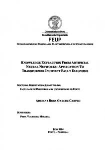
% All the neurons have initially the same weights in the %middle of the vectors plotsom(som.iw{1,1},som.layers{1}.distances) % after training, the layer of neurons has begun to self%organize % Each neuron classifies a different region of the input space % adjacent (connected) neurons respond to adjacent %regions. net.trainParam.epochs = 100; somt = train(som,X); plotsom(somt.iw{1,1},somt.layers{1}.distances) display(som.iw{1,1}); % using sim to classify vectors by giving them to the %network % neuron "y" responded with a "1", so “test” belongs to %that class. test = [0.1;0.5]; y = sim(somt,test) Here is what the self-organizing map looks like before training:
Fig.1: Before training Here is what the self-organizing map looks like after 1000 epochs of training:
Fig.2: After 1000 epochs of training After training process map is more evenly distributed across the input space. The weights of neurons and the result of the classification displayed in the command window are: weights = -0.7805 -0.6823 -0.7690 -0.4027 -0.7767 -0.0035
-0.7681 0.3984 -0.7218 0.6952 -0.5250 -0.6942 -0.5320 -0.3897 -0.5260 -0.0852 -0.4508 0.4013 -0.4195 0.7436 -0.1549 -0.7265 -0.2026 -0.4436 -0.1490 -0.0263 -0.1150 0.4703 -0.1246 0.7537 0.1202 -0.7022 0.1030 -0.3672 0.1501 -0.0260 0.1515 0.4201 0.1169 0.7446 0.4621 -0.7398 0.4707 -0.4103 0.4339 0.0076 0.4353 0.3642 0.4566 0.7146 0.7226 -0.7031 0.7622 -0.4325 0.7085 -0.0848 0.7067 0.3999 0.6909 0.7136 y= (19,1) 1 The self-organizing map weight learning function is learnsom. The network identifies the winning neuron first and then, the weights of the winning neuron and the other neurons in its neighborhood are moved closer to the input vector at each learning step using the self-organizing map learning function. During training the learning rate and the neighborhood distance used to determine which neurons are in the winning neuron’s neighborhood are altered through two phases: ordering and tuning phase. In ordering phase which lasts for the given number of steps the neighborhood distance starts as the maximum distance between two neurons, and decreases to the tuning neighborhood distance. On the other hand the learning rate starts at the ordering-phase learning rate and decreases until it reaches the tuning-phase learning rate. As the neighborhood distance and learning rate decrease over this phase, the neurons of the network typically order themselves in the input space with the same topology in which they are ordered physically. In tuning phase which lasts for the rest of training or adaption the neighborhood distance stays at the tuning neighborhood distance, (which should include only close neighbors , typically 1.0). The learning rate continues to decrease from the tuning phase learning rate, but very slowly. The small neighborhood and slowly decreasing learning rate fine-tune the network, while keeping the ordering learned in the previous phase stable. The number of epochs for the tuning part of training (or time steps for adaptation) should be much larger than the number of steps in the ordering phase, because the tuning phase usually takes much longer.
CONCLUSIONS As with competitive layers, the neurons of a selforganizing map will order themselves with approximately equal distances between them if input vectors appear with even probability throughout a section of the input space. Also, if input vectors occur with varying frequency throughout the input space, the feature map layer tends to allocate neurons to an area in proportion to the frequency of input vectors there. Self-organizing maps differ from conventional competitive learning in terms of which neurons get their weights updated: instead of updating only the winner, feature maps update the weights of the
winner and its neighbors, so the neighboring neurons tend to have similar weight vectors and to be responsive to similar input vectors. After the training process the map is rather evenly spread across the input space. REFERENCES Dumitrescu D., 2003, Principiile inteligentei artificiale, Editura Albastra, Cluj Napoca Nastac D. I., 2002, Retele neuronale artificiale, Editura Printech, Bucuresti http://www.mathworks.com http://www.math.uvt.ro