Label-Guided Graph Exploration by a Finite Automaton∗ Reuven Cohen † Pierre Fraigniaud ‡ David Ilcinkas Amos Korman § David Peleg ¶
‡
May 26, 2006 Abstract A finite automaton, simply referred to as a robot, has to explore a graph, i.e., visit all the nodes of the graph. The robot has no a priori knowledge of the topology of the graph or of its size. It is known that, for any k-state robot, there exists a (k + 1)node graph of maximum degree 3 that the robot cannot explore. This paper considers the effects of allowing the system designer to add short labels to the graph nodes in a preprocessing stage, and using these labels to guide the exploration by the robot. We describe an exploration algorithm that given appropriate 2-bit labels (in fact, only 3valued labels) allows a robot to explore all graphs. Furthermore, we describe a suitable labeling algorithm for generating the required labels, in linear time. We also show how to modify our labeling scheme so that a robot can explore all graphs of bounded degree, given appropriate 1-bit labels. In other words, although there is no robot able to explore all graphs of maximum degree 3, there is a robot R, and a way to color in black or white the nodes of any bounded-degree graph G, so that R can explore the colored graph G. Finally, we give impossibility results regarding graph exploration by a robot with no internal memory (i.e., a single state automaton). ∗
A preliminary version appeared in Proc. 32nd Int. Colloq. on Automata, Languages and Programming. Dept. of Electrical and Computer Eng., Boston University, Boston, MA, USA. E-mail:
[email protected]. Supported by the Pacific Theaters Foundation. ‡ CNRS, LRI, Universit´e Paris-Sud, France. E-mail: {pierre,ilcinkas}@lri.fr. Supported by the project “PairAPair” of the ACI Masses de Donn´ees, the project “Fragile” of the ACI S´ecurit´e et Informatique, and by the project “Grand Large” of INRIA. § Information Systems Group, Faculty of IE&M, The Technion, Haifa, Israel. E-mail: pandit@ tx.technion.ac.il. Supported in part by an Aly Kaufman fellowship. ¶ Dept. of Computer Science, The Weizmann Institute, Rehovot, Israel. E-mail: david.peleg@ weizmann.ac.il. Supported in part by a grant from the Israel Science Foundation. †
1
Introduction
Background: This paper concerns graph exploration by finite automata. Let R be a finite automaton, simply referred to in this context as a robot, moving in an unknown graph G = (V, E). The robot has no a priori information about the topology of G and its size. To allow the robot R to distinguish between the different edges of a node u while visiting it, the d = deg(u) edges incident to u are associated with d distinct port numbers in {0, . . . , d − 1}, in a one-to-one manner. The port numbering is given as part of the input graph, and the robot has no a priori information about it. For convenience of terminology, we henceforth refer to the edge incident to port number l at node u simply as “edge l of u”. (Clearly, if this edge connects u to v, then it may also be referred to as “edge l′ of v” for the appropriate l′ .) The robot has a finite number of states and a transition function f . If R enters a node of degree d through port i in state s, then it switches to state s′ and exits the node through port i′ , where (s′ , i′ ) = f (s, i, d). The objective of the robot is to explore the graph, i.e., to visit all its nodes. The first known algorithm designed for graph exploration was introduced by Shannon [9]. Since then, several papers have been dedicated to the feasibility of graph exploration by a finite automaton. Rabin [7] conjectured that no finite automaton with a finite number of pebbles can explore all graphs (a pebble is a marker that can be dropped at and removed from nodes). The first step towards a formal proof of Rabin’s conjecture is generally attributed to Budach [2], for a robot without pebbles. Blum and Kozen [1] improved Budach’s result by proving that a robot with three pebbles cannot perform exploration of all graphs. Kozen [6] proved that a robot with four pebbles cannot explore all graphs. Finally, Rollik [8] gave a complete proof of Rabin’s conjecture, showing that no robot with a finite number of pebbles can explore all graphs. The result holds even when restricted to planar 3-regular graphs. Without pebbles, it was proved [5] that a robot needs Θ(D log ∆) bits of memory for exploring all graphs of diameter D and maximum degree ∆. On the other hand, if the class of input graphs is restricted to trees, then exploration is possible even by a robot with no memory (i.e., zero states), simply by depth-first search (DFS) using the transition function f (i, d) = i + 1 mod d (see, e.g., [4]). Label-guided exploration: The ability of dropping and removing pebbles at nodes can be viewed alternatively as the ability of the robot to dynamically label the nodes. If the robot is P given k pebbles, then at any time during the exploration, u∈V |lu | ≤ k, where lu is the label of node u and |lu | denotes the size of the label in unary. In certain settings, it is expected that the graph will be visited by many exploring robots, 1
and consequently, it is desired to preprocess the graph by leaving fixed (preferably small) roadsigns, or labels, that will aid the robots in their exploration task. As a possible scenario, one may consider a network system where finite automata are used for traversing the system and distributing information in a sequential manner. This paper considers the effects of allowing the system designer to assign labels to the nodes in a preprocessing stage, and using these labels to guide robot explorations. The transition function f is augmented to utilize labels as follows. If R in state s enters a node of degree d, labeled by l, through port i, then it switches to state s′ and exits the node through port i′ , where (s′ , i′ ) = f (s, i, d, l). This model can be considered stronger than Rabin’s pebble model since labels are given in a preprocessing stage, but it can also be considered weaker since, once assigned to nodes, the labels cannot be modified1 . More formally, we address the design of exploration labeling schemes. Such schemes consist of a pair (L, R) such that, given any graph G with any port numbering, the algorithm L labels the nodes of G, and the robot R explores G with the help of the labeling produced by L. In particular, we are interested in exploration labeling schemes for which: (1) the preprocessing time required to label the nodes is polynomial, (2) the labels are short, and (3) the exploration is completed after a small number of edge traversals. Our results: As a consequence of Rollik’s result, any exploration labeling scheme must use at least two different labels. Our main result states that just three labels (e.g., three colors) are sufficient for enabling a robot to explore all graphs. Moreover, we show that our labeling scheme gives to the robot the power to stop once exploration is completed, although, in the general setting of graph exploration, the robot is not required to stop once the exploration has been completed, i.e., once all nodes have been visited. In fact, we show that exploration is completed in time O(m), i.e., after O(m) edge traversals, in any m-edge graph. For the class of bounded degree graphs, we design an exploration scheme using even smaller labels. More precisely, we show that just two labels (i.e., 1-bit labels) are sufficient for enabling a robot to explore all bounded degree graphs. The robot is however required to have a memory 1
It should be noted that the general function presented here may depend on d, i and l, all of which may require log N bits to describe on an N node graph. However, the algorithm suggested in this paper actually allows only three possible outputs: i′ = i and i′ = i ± 1(modd), which can be interpreted as ‘go left”, “go right”, and “go back” commands. The output of the algorithm among these three depends only on the state and the only dependence on l and i is in the case they equal 0. Therefore, it can be considered to be a real fixed memory algorithm.
2
Label size (#bits) 2 1
Robot’s memory (#bits) O(1) O(log ∆)
Time (# edge traversals) O(m) O(∆O(1) m)
Table 1: Summary of main results. of size O(log ∆) to explore all graphs of maximum degree ∆. The completion time O(∆O(1) m) of the exploration is larger than the one of our previous 2-bit labeling scheme, nevertheless it remains polynomial. All these results are summarized in Table 1. The two mentioned labeling schemes require polynomial preprocessing time. We also prove several impossibility results for 1-state (i.e., oblivious) robots. The behavior of 1-state robots depends solely on the input port number, and on the degree and label of the current node. In particular, we prove that for any d > 4 and for any 1-state robot using at most ⌊log d⌋ − 2 colors, there exists a simple graph of maximum degree d that cannot be explored by the robot. This lower bound on the number of colors needed for exploration can be increased exponentially to d/2 − 1 by allowing loops.
2 2.1
A 2-bit exploration-labeling scheme Exploration with pre-labeling
In this section, we describe an exploration-labeling scheme using only 2-bit (actually, 3-valued) labels. More precisely, we prove the following. Theorem 2.1 There exists a robot with the property that for any m-edge graph G, it is possible to color the nodes of G with three colors (or alternatively, assign each node a 2-bit label) so that using the labeling, the robot can explore the graph G, starting from any given node and terminating after identifying that the entire graph has been traversed. Moreover, the total number of edge traversals by the robot is at most 20m. To prove Theorem 2.1, we first describe the labeling scheme L and then the exploration algorithm. The node labeling is in fact very simple, and uses three colors denoted white, black, and red. Let D denote the diameter of the graph.
3
Labeling L. Pick an arbitrary node r to be the root of the labeling L. Nodes at distance d from r, 0 ≤ d ≤ D, are labeled white if d mod 3 = 0, black if d mod 3 = 1, and red if d mod 3 = 2. The neighbor set N (u) of each node u can be partitioned into three disjoint sets: (1) the set pred(u) of neighbors closer to r than u; (2) the set succ(u) of neighbors farther from r than u; (3) the set sibling(u) of neighbors at the same distance from r as u. We also identify the following two special subsets of neighbors: • parent(u) is the node v ∈ pred(u) such that the edge {u, v} has the smallest port number at u among all edges connecting it to a node in pred(u). • child(u) is the set of nodes v ∈ succ(u) such that parent(v) = u. For the root, set parent(r) = ∅. The exploration algorithm is partially based on the following observations. 1. For the root r, child(r) = succ(r) = N (r). 2. For every node u with label L(u), and for every neighbor v ∈ N (u), the label L(v) uniquely determines whether v belongs to pred(u), succ(u) or sibling(u). 3. Once at node u, a robot can identify parent(u) by visiting its neighbors successively, starting with the neighbor connected to port 0, then port 1, and so on. Indeed, by observation 2, the nodes in pred(u) can be identified by their label. The order in which the robot visits the neighbors ensures that parent(u) is the first visited node in pred(u). Observe that one of the main difficulties of graph exploration by a robot with a finite memory is that the robot entering some node u by port p, and aiming at exiting u by the same port p after having performed some local exploration around u, does not have enough memory to store the value of p. Exploration algorithm. Our exploration algorithm uses a procedure called Check Edge. This procedure is specified as follows. When Check Edge(j) is initiated at some node u, the robot starts visiting the neighbors of u one by one, and eventually returns to u reporting one of three possible outcomes: “child”, “parent”, or “false”. These values have the following interpretation: 4
(i) if “child” is returned, then edge j at u leads to a child of u; (ii) if “parent” is returned, then edge j at u leads to the parent of u; (iii) if “false” is returned, then edge j at u leads to a node in N (u) \ (parent(u) ∪ child(u)). The implementation of Procedure Check Edge will be described later. Meanwhile, let us describe how the algorithm makes use of this procedure to perform exploration. In this description, all arithmetic operations are modulo d. Assume that the robot R is initially at the root r of the 3-coloring L of the nodes. R leaves r by port number 0, in state down. Note that, by the above observations, the node at the other endpoint of edge 0 of r is a child of r. Now assume that R enters a node u of degree d via port number i. If R is in state down, then it aims at identifying a child of u if one exists, or to backtrack along edge i of u if none exists. If R is in state up, then it aims at identifying a child of u with port number j ∈ {i + 1, . . . , p − 1} if one exists (where p is the port number of the edge leading to parent(u)), or to carry on moving up to the parent of u if there is no such child. In both cases, R achieves its goal as follows. R executes Procedure Check Edge(j) for every port number j = i + 1, i + 2, . . . until the procedure eventually returns “child” or “parent” for some port number j. R then sets its state to down in the former case and up in the latter, and leaves u by port j. If the robot does not start from the root r of the labeling L, then it first goes to r by using Procedure Check Edge to identify the parent of every intermediate node, and by identifying r as the only node with pred(r) = ∅. Moreover, the robot can stop after the exploration has been completed. More precisely, this can be done by introducing a slight modification of the robot behavior when it enters a node u of degree d via port number d in state up. In this case, R first check whether u has a parent. If yes, then it acts as previously stated (R does not need to store d since d is the node degree). If not, the robot terminates the exploration. Procedure Check Edge. We now describe the actions of the robot R when Procedure Check Edge(j) is initiated at a node u. The objective of R is to set the value of the variable edge to one of {parent, child, false}. We denote by v the other endpoint of the edge e with port number j at u. First, R moves to v in state “check edge”, carrying with it the color of node u. Let i be the port number of edge e at v. There are three cases to be considered. 5
(a) v ∈ sibling(u): Then R backtracks through port i and reports “edge = false”. (b) v ∈ pred(u): Then R aims at checking whether v is the parent of u, that is, whether u is a child of v. For that purpose, R moves back to u, and proceeds as follows: R successively visits edges j − 1, j − 2, . . . of u until either the other endpoint of the edge belongs to pred(u), or all edges j −1, j −2, . . . , 0 have been visited. R then sets “edge=false” in the former case and “edge=parent” in the latter. At this point, let k be the port number at u of the last edge visited by R. Then R successively visits edges k + 1, k + 2, · · · until the other endpoint belongs to pred(u). Then it moves back to u and reports the value of edge. (c) v ∈ succ(u): Then R aims at checking whether u is the parent of v. For that purpose, R proceeds in a way similar to Case (b), i.e., it successively visits edges i − 1, i − 2, . . . of v until either the other endpoint of the edge belongs to pred(v), or all edges i−1, i−2, . . . , 0 have been visited. R then sets its variable edge to “false” in the former case and to “child” in the latter. At this point of the exploration, let k denote the port number of the last edge incident to v that R visited. Then R successively visits edges k + 1, k + 2, . . . until the other endpoint w of the edge belongs to pred(v). Then it moves to w and reports the value of edge. This completes the description of our exploration procedure. Proof of Theorem 2.1. Clearly, all nodes of an m-edge graph can be labelled by L, using two bits per label, in time linear in m. It remains to prove the correctness of the exploration algorithm. It is easy to check that if Procedure Check Edge satisfies its specifications, then the robot R essentially performs a DFS traversal of the graph using edges {u, v} where u = parent(v) or u ∈ child(v). Thus, we focus on the correctness of Procedure Check Edge(j) initiated at node u. Let v be other endpoint of the edge e with port number j at u, and let i be the port number of edge e at v. We check separately the three cases considered in the description of the procedure. By the previous observations, comparing the color of the current node with the color of u allows R to distinguish between these cases. If v ∈ sibling(u), then v is neither a parent nor a child of u, and thus reporting “false” is correct. Indeed, R then backtracks to u via port i, as specified in Case (a). If v ∈ pred(u), then v = parent(u) iff for every neighbor wk connected to u by an edge with port number k ∈ {j − 1, j − 2, . . . , 0}, wk ∈ / pred(u). The robot does check this property
6
in Case (b) of the description, by returning to u, and visiting all the wk ’s. Hence, Procedure Check Edge performs correctly in this case. Finally, if v ∈ succ(u), then v = child(u) iff for every neighbor zl connected to v by an edge with port number l ∈ {i − 1, i − 2, . . . , 0}, zl ∈ / pred(v). In case (c), the robot does check this property by visiting all these neighbors zl . At this point, it remains for R to return to u (obviously, the port number leading from v to u cannot be stored in the robot’s memory since it has only a constant number of states). Let k be the port number of the last edge incident to v that R visited before setting its variable edge to “false” or “child”. We have 0 ≤ k ≤ i − 1, zl ∈ / pred(v) for all l ∈ {k + 1, . . . , i − 1}, and u ∈ pred(v). Thus u is identified as the first neighbor that is met when visiting all v’s neighbors by successively traversing edges k + 1, k + 2, . . . of v. This is precisely what R does according to the description of the procedure in Case (c). Hence, Procedure Check Edge performs correctly in this case. In summary, Procedure Check Edge performs correctly in all cases and so does the global exploration algorithm. It remains to compute the number of edge traversals performed by the robot during the exploration (including the calls to Check Edge). We use again the same notations as in the description and the proof of Procedure Check Edge. Let us consider the Procedure Check Edge(j) initiated at node u. Let v be other endpoint of the edge e with port number j at u, and let i be the port number of edge e at v. First observe that during the execution of the Procedure Check Edge only edges incident to u and v are traversed. More precisely: Case (a): v ∈ sibling(u). Then edge e = {u, v} is traversed twice and no other edges are traversed during this execution of Procedure Check Edge. Case (b): v ∈ pred(u). Then R traverses only edges incident to u. Let k be the greatest port number of the edges leading to a node in pred(u) and satisfying k < j. If it does not exist, set k = 0. R explores twice each edge j, j − 1, . . . , k + 1 of u, then twice edge k, and finally again twice edges k + 1, . . . , j − 1, j. To summarize, edge k of u is explored twice, and edges k + 1, . . . , j − 1, j of u are explored four times. Case (c): v ∈ succ(u). Then R traverses only edges incident to v. Let k be the greatest port number of the edges leading to a node in pred(v) and satisfying k < i. If it does not exist, set k = 0. R explores once edge j of u, twice each edge i − 1, i − 2, . . . , k + 1 of v, twice edge k, twice again edges k + 1, . . . , i − 2, i − 1, and finally once edge i of v (i.e., j of u). To summarize, edge i of u and edge k of v are explored twice and edges k + 1, . . . , i − 2, i − 1 of v are explored four times.
7
v’
(1),(2)
(3)
j’’
j’
u’
u’
v’
i’’
j’’
i’
j’
v i’’
j
u i’
i
j
v
i
u
Figure 1: Notations for case (1), (2) and (3) of the analysis We bound now the number of times each edge e of the graph is traversed. Edge e = {u, v} is labeled i at u and j at v. Let us consider different cases (see Figure 1): (1) e = {u, v} with v = parent(u). The edge e is in the spanning tree, and thus is explored twice outside any execution of the Procedure Check Edge. During Procedure Check Edge(j) at v, edge e is explored twice. e is also explored four times during Check Edge(i) at u, except if i = 0 where e is only explored twice during Check Edge(i) at u. If there exists an edge {u′, u} labeled i′ at u and i′′ at u′ such that i′ < i and u′ ∈ pred(u), then edge e is explored twice during Procedure Check Edge(i′ ) at u and twice again during Procedure Check Edge(i′′ ) at u′ . If there exists an edge {v ′, v} labeled j ′ at v and j ′′ at v ′ such that j ′ < j and v ′ ∈ pred(v), then edge e is explored four times during Procedure Check Edge(j ′ ) at v and four times again during Procedure Check Edge(j ′′ ) at v ′ . To summarize, edge e is explored at most 20 times during a DFS. (2) e = {u, v} with v ∈ pred(u) but v 6= parent(u). During Procedure Check Edge(j) at v, edge e is explored twice. e is also explored four times during Check Edge(i) at u. If there exists an edge {u′ , u} labeled i′ at u and i′′ at u′ such that i′ < i and u′ ∈ pred(u), then edge e is explored twice during Procedure Check Edge(i′ ) at u and twice again during Procedure Check Edge(i′′ ) at u′ . If there exists an edge {v ′, v} labeled j ′ at v and j ′′ at v ′ such that j ′ < j and v ′ ∈ pred(v), then edge e is explored four times during Procedure Check Edge(j ′ ) at v and four times again during Procedure Check Edge(j ′′ ) at v ′ . To summarize, edge e is explored at most 18 times during a DFS. (3) e = {u, v} with v ∈ sibling(u). During Procedure Check Edge(j) at v, edge e is explored twice. e is also explored twice during Check Edge(i) at u. If there exists an edge {u′ , u} labeled i′ at u and i′′ at u′ such that i′ < i and u′ ∈ pred(u), then edge e is explored four times during Procedure Check Edge(i′ ) at u and four times again during Procedure Check Edge(i′′ ) at u′ . If there exists an edge {v ′ , v} labeled j ′ at v and j ′′ at v ′ such 8
that j ′ < j and v ′ ∈ pred(v), then edge e is explored four times during Procedure Check Edge(j ′ ) at v and four times again during Procedure Check Edge(j ′′ ) at v ′ . To summarize, edge e is explored at most 20 times during a DFS. Therefore, our exploration algorithm completes exploration in time at most 20|E| where |E| is the number of edges in the graph G.
2.2
Exploration while labeling
The above description assumes that the labeling of the graph was conducted by an external entity prior to the exploration process by the robot. As an alternative, we present here a minor change to the exploration algorithm, allowing the robot to color the graph while conducting the exploration process. For simplicity, we assume that all nodes begin at an uncolored “blank” state, and that the robot can identify such blank nodes. Alternatively, one can assume that blank represents a forth color, making this a full 2-bit scheme. For the coloring process, the robot needs three extra bits of memory: a flag have colored and a 2-bit variable next color. At the beginning of the exploration, the robot colors its current location white, sets next color to black and clears have colored. The exploration proceeds in successive phases. The objective of phase i ≥ 0 is to color all nodes at distance i from r. More precisely, letting Gi be the subgraph of the explored graph G induced by all nodes at distance at most i from the root r, the specification P (i) of phase i states that the robot starts phase i from the root, traverses all the edges of Gi , colors all blank nodes by the color next color of the phase, and returns to the root. For this purpose, we modify the procedure Check Edge as follows. Assume Check Edge is called at node u for some edge e incident to u. The procedure proceeds the same as before, except that whenever the robot traverses an edge {x, y} from a colored node x to a blank node y, the following rules are applied: • If the color of x is different from next color, then y is colored by next color, and the procedure carries on the same way as if y was already colored next color when the robot entered it; • Otherwise (i.e., the color of x is next color), the robot returns to x and carries on just as if the edge {x, y} did not exist. Whenever a node is colored next color, the flag have colored is set to true. 9
The exploration process is also changed, such that whenever the exploration should have stopped in the original algorithm, the robots now checks if the flag have colored is set, and if so, clears it, sets next color ← succ(next color), and restarts the exploration. Otherwise, it stops. Theorem 2.2 By the end of the execution of the modified algorithm, the graph is fully colored and the robot has explored the entire graph, terminating at the root. Proof: We have to show that the algorithm meets its specification P (i) for eevry i ≥ 0. This is done by induction on the phase i. P (0) holds by construction. For i ≥ 1, assume that P (i − 1) holds and let us prove P (i). Define the layer i of G as the set of nodes at distance exactly i from r. By the inductive hypothesis, all nodes of Gi−1 are colored properly, i.e., according to the labeling L of the previous section. Whenever the robot colors a node u during phase i, it has arrived from a node v that is colored and whose color is not next color. Therefore v belongs to layer i − 1, and u is colored by the proper color next color. By the modification of procedure Check Edge, whenever a non-colored node of layer i is visited by the robot coming from another node of layer i, the robot backtracks immediately. Therefore, every time the robot reaches a node u of layer i + 1, it comes from a colored node v of layer i. Since v is properly colored next color, u is not colored, and the robot backtracks, ignoring edge {u, v}. Therefore, the global behavior of the robot in G at phase i is the same as its behavior in the graph Gi at the same phase i. In fact, there is only one difference that occurs between siblings at layer i. In this situation, the modified procedure Check Edge backtracks and may ignore the edge. However, this has no impact on the exploration since anyway, even if all the nodes are colored a priori, the robot always backtracks when visiting a sibling. By Theorem 2.1, all the edges of Gi will be traversed, and the robot will return to the root. In fact, let T be the spanning tree of the explored graph G as induced by the labeling L of the previous section, and for i ≥ 0 let Ti be the subtree of T spanning all nodes at distance at most i from the root r. The exploration proceeds as a DFS traversal of Ti , thus all node of layer i are visited from a node of layer i − 1, and hence are properly colored with next color. Hence P (i) holds. It follows that after D phases (where D is the diameter of the graph), the robot has completed coloring all nodes of the graph and has explored the entire graph. Nevertheless, yet another phase is performed, in which the robot discovers that the exploration and the coloring are actually completed.
10
3
A 1-bit exploration-labeling scheme for bounded degree graphs
In this section, we describe an exploration labeling scheme using only 1-bit labels. This scheme requires a robot with O(log ∆) bits of memory for the exploration of graphs of maximum degree ∆. More precisely, we prove the following. Theorem 3.1 There exists a robot with the property that for any graph G of degree bounded by a constant ∆, it is possible to color the nodes of G with two colors (or alternatively, assign each node a 1-bit label) so that using the labeling, the robot can explore the graph G, starting from any given node and terminating after identifying that the entire graph has been traversed. The robot has O(log ∆) bits of memory, and the total number of edge traversals by the robot is O(∆O(1) m). To prove Theorem 3.1, we first describe a 1-bit labeling scheme L′ for G = (V, E), i.e., a coloring of each node in black or white. Then, we show how to perform exploration using L′ . Labeling L′ . As for the labeling L of the previous section, pick an arbitrary node r ∈ V , called the root. Nodes at distance d from r are labeled as a function of d mod 8. Denote the distance between two nodes v and u in G by distG (v, u). Partition the nodes into eight classes by letting Ci = {u ∈ V | distG (r, u) mod 8 = i} for 0 ≤ i ≤ 7. Node u is colored white if u ∈ C0 ∪ C2 ∪ C3 ∪ C4 , and black otherwise. Let C˜1 = {u | distG (r, u) = 1} b = {r} ∪ {u ∈ C2 | distG (r, u) = 2 and N (u) = C˜1 }. C Lemma 3.2 There is a local search procedure enabling a robot of O(log ∆) bits of memory to b and to C˜1 , and to identify the class Ci of every node decide whether a node u belongs to C b u∈ / C. Proof: Let B (resp., W) be the set of black (resp., white) nodes all of whose neighbors are also black (resp., white). One can easily check that the class C1 and the classes C3 , . . . , C7 can be redefined as follows: • u ∈ C6 ⇔ u ∈ B and there is a node in W at distance at most 3 from u; 11
• u ∈ C7 ⇔ u ∈ / C6 , u has a neighbor in C6 , and there is no node in W at distance at most 2 from u; • u ∈ C1 ⇔ u is black, u has no neighbor in B, and u has a white neighbor v that has no neighbor in W. • u ∈ C5 ⇔ u is black, and u ∈ / C1 ∪ C6 ∪ C7 ; • u ∈ C3 ⇔ u ∈ W, and there is a node in C1 at distance at most 2 from u; • u ∈ C4 ⇔ u has a neighbor in W, and there is no node in C1 at distance at most 2 from u. Based on the above characterizations, the classes C1 and C3 , . . . , C7 can be easily identified b can by a robot of O(log ∆) bits, via performing a local search. Moreover, the sets C˜1 and C also be characterized as follows: • u ∈ C˜1 ⇔ u ∈ C1 and there is no node in C7 at distance at most 2 from u; b ⇔ N(u) ⊆ C˜1 and every node v at distance at most 2 from u satisfies |N(v)∩C˜1 | ≤ • u∈C |N(u)|. Using this we can deduce: b⇔u∈ • u ∈ C0 \ C / (∪7i=3 Ci ) ∪ C1 and u has a neighbor in C7 ; b⇔u∈ b u has a neighbor in C1 but no neighbor in C7 . • u ∈ C2 \ C / C, It follows that a robot of O(log ∆) bits can identify the class of every node except for nodes b in C. Proof of Theorem 3.1. The exploration algorithm for L′ follows the same strategy as the exploration algorithm for L. Indeed, for u ∈ Ci we have pred(u) = N (u) ∩ Ci−1 succ(u) = N (u) ∩ Ci+1 sibling(u) = N (u) ∩ Ci .
(mod 8) , (mod 8) ,
Therefore, due to Lemma 3.2, all instructions of the exploration algorithm using labeling L b can be executed using labeling L′ , but for the cases not captured in Lemma 3.2, i.e., C. 12
b can be To solve the problem of identifying the root, we notice that each of the nodes in C used as a root, and all the others can be considered as leaves in C2 . Thus, when leaving the root, the robot should memorize the port P by which it should return to the root. When the robot arrives at a node u ∈ C˜1 through a tree edge and is in the up state, it leaves immediately through port P and deletes the contents of P , then it goes down through the next unexplored port if one is left. When the robot is in a node u ∈ C˜1 and in the down state, it will skip the port P . If the exploration begins at the root, then the above is sufficient. To handle explorations b can beginning at an arbitrary node, it is necessary to identify the root. Since every node in C b by going up, and then start the exploration be used as a root, it suffices to find one node of C from it as described above.
4
Impossibility results
Theorem 4.1 For any d > 4, and for any 1-state robot using at most d/2 − 1 colors, there exists a graph (with loops) with maximum degree d and at most d+1 vertices that cannot be explored by the robot. Proof: Fix d > 4, and assume for contradiction that there exists a 1-state robot exploring all graphs of degree d colored with at most d/2 − 1 colors. Recall that when a 1-state robot enters a node v by port i, it will leave v by port j where j is depending only on i, d and the color c of v. Thus for fixed d, each color corresponds to a mapping from entry ports to exit ports, namely, a function from {0, 1, · · · , d − 1} to {0, 1, · · · , d − 1}. Partition the functions corresponding to the colors of nodes of degree d into surjective functions f1 , f2 , · · · , ft and non-surjective functions g1 , g2, · · · , gr . We have 0 < t + r ≤ d/2 − 1. Let ci be the color corresponding to fi , and ct+i be the color corresponding to gi . For each gi , choose pi to be some port number not in the range of gi . Let p0 ∈ {0, 1, · · · , d − 1} \ {p1 , p2 , · · · , pr } (it is possible because d − r ≥ 1). We construct a family {G0 , G1 , · · · , Gt } of graphs such that, for every k ∈ {0, 1, · · · , t}: 1. Gk has exactly one degree-d vertex v (possibly with loops); 2. the other vertices of Gk are degree-1 neighbors of v; 3. all edges are either loops incident to v, or edges leading from v to some degree-1 node; 4. edges labeled p1 , p2 , · · · , pr at v (if any, i.e., if r > 0) are not loops (and thus lead to degree-1 nodes); 13
5. the edge labeled p0 leads to some degree-1 node, denoted by u0 ; 6. there exists a set Xk ⊆ {0, 1, · · · , d − 1} such that {p0 , p1 , · · · , pr } ⊆ Xk and d − |Xk | > 2(t − k), and for which, in Gk , edges with port number not in Xk lead to degree-1 vertices. We prove the following property for any k = 0, · · · , t: Property Pk . In Gk , if the color of v is in {c1 , · · · , ck }, then the robot, starting at u0 ∈ V (Gk ), cannot explore Gk . More precisely any vertex attached to v by a port 6∈ X is not visited by the robot. We prove Pk by induction on k. Let G0 be the star composed of one degree-d vertex v and d leaf vertices. Let X0 = {p0 , p1 , p2 , · · · , pr }. Recall that t + r ≤ d/2 − 1. Thus, t ≤ d/2 − 1 and hence 2t + r + 1 ≤ d − 1. Therefore, we have d − |X0 | = d − (r + 1) > 2t. P0 is trivially true. Let k > 0, and let Gk−1 and Xk−1 be respectively a graph and a set satisfying the induction property for k − 1. Assume first that v is colored by color ck and that the robot starts its traversal at u0 . If the robot never visits vertices attached to v by ports not in Xk−1 then the graph Gk−1 and the set Xk−1 satisfy Pk . I.e., Gk = Gk−1 and Xk = Xk−1 . Otherwise, let p be the first port not in Xk−1 that is visited by the robot at v, when starting at u0 . For a port i ∈ {0, 1, · · · , d − 1}, set twin(i) = j if there exists a port j and a loop labeled by i and j in Gk−1 ; Set twin(i) = i otherwise. Define a sequence of ports (il )l≥1 as follows. Let i1 be the port in Xk−1 such that fk (i1 ) = p. For all l ≥ 2, let il be the port such that fk (il ) = twin(il−1 ). This sequence is well defined because fk is surjective. Observe that there exists some l such that il ∈ / Xk−1 . Indeed, suppose, for the purpose of contradiction, that il ∈ Xk−1 for all l. Since Xk−1 is finite, there exists some il = il+m for m ≥ 1. Let il be the first port repeated twice in this process. If l > 1, then we have fk (il ) = twin(il−1 ) and fk (il+m ) = twin(il+m−1 ). Therefore twin(il−1 ) = twin(il+m−1 ), yielding il−1 = il+m−1 by bijectivity of fk , which contradicts the minimality of l. If l = 1, then we have i1 = i1+m , therefore im = p, contradicting ij ∈ Xk−1 for all j. From the above, let h be the smallest index such that ih ∈ / X. Let q = ih . If q = p, then set Gk = Gk−1 and Xk = Xk−1 ∪ {p}. If q 6= p, then connect ports p and q to create a loop, denote the new graph Gk and let Xk = Xk−1 ∪ {p, q}. In Gk , if v is colored by color ck , then by the choice of p, starting at u0 , the robot enters and exits v through ports in Xk−1 until it eventually exits v through port p. After that, the robot 14
goes back to v by port q. Port q was chosen so that it causes the robot to continue entering v on ports ih−1 , ih−2 , · · · i1 , after which the robot exits v through port p, locking the robot in a cycle. Since the ports of v occurring in this cycle are all from Xk , the robot does not visit any of the ports outside Xk , as claimed. By induction, we have d − |Xk−1| > 2(t − (k − 1)). By the construction of Xk from Xk−1 , we have |Xk | ≤ |Xk−1 | + 2. Therefore d − |Xk | > 2(t − k), which completes the correctness of Gk and Xk . If the color of v in Gk is in {c1 , · · · , ck−1} then the robot is doomed to fail in exploring Gk . Indeed since starting at u0 in Gk−1 the robot does not traverse any of the vertices corresponding to ports not in Xk−1 , then in Gk too, the robot does not traverse any of the vertices corresponding to ports not in Xk ⊇ Xk−1 , and thus fails to explore Gk because d − |Xk | ≥ 1. This completes the proof of Pk and thus the induction. In particular, Gt is not explored by the robot if the node v is colored with a color in c1 , c2 , · · · , ct . If v is colored ct+i with 1 ≤ i ≤ r, then assume that the robot starts the traversal at vertex u0 . Since the edge labeled pi leads to a degree-1 vertex in Gt , this vertex will never be visited by the robot, by definition of pi . Therefore the graph Gt cannot be explored by the robot. The theorem above makes use of graphs with loops. For graphs without loops we have the following theorem. Theorem 4.2 For any d > 4 and for any 1-state robot using at most ⌊log d⌋ − 2 colors, there exists a graph of maximum degree d, without loops, that cannot be explored by the robot. Proof: As in the proof of Theorem 4.1, denote the functions corresponding to the colors by f1 , f2 , · · · , ft , g1 , g2, · · · , gr where the fi ’s are surjective functions and the gi’s are non-surjective ones. For each gi , choose pi to be some port number not in the range of gi . We use the same proof as for Theorem 4.1, except that we replace each loop L of the construction in there by a loopless graph. For a loop L of vertex v, with port numbers i and j, let GL be the following graph. Connect v by edges to two new vertices w and w ′ , add the edge (w, w ′), and connect w (respectively, w ′ ) to d−2 new vertices n1 , n2 , · · · , nd−2 (resp., n′1 , n′2 , · · · , n′d−2 ). We now set the port numbering for GL . Assign the port numbers i and j for the edges (v, w) and (v, w ′ ). At w (respectively, w ′ ) use the port numbers p1 , p2 , · · · , pr for the edges (w, n1), (w, n2 ), · · · , (w, nr ) (resp., (w ′, n′1 ), (w ′, n′2 ), · · · , (w ′, n′r )). The port numbers p and q that w uses for the edges (w, v) and (w, w ′) are the same as the port numbers that w ′ uses for the edges (w ′ , v) and (w ′ , w). They are chosen in a particular way from the set {0, 1, · · · , d − 1} \ {p1 , p2 , · · · , pr } to be specified later. We immediately get that w and w ′ cannot be colored by a color whose corresponding function is in the set g1 , g2 , · · · , gr since these functions are not surjective and ports {p1 , p2 , · · · , pr } lead to leaves of w and w ′ . To complete the proof, we claim the following: 15
Claim: There exist two ports p, q ∈ {0, 1, · · · , d − 1} \ {p1 , p2 , · · · , pr } such that if the robot enters either w or w ′ by port p (respectively, q), then if some time later the robot exits through the same port p (resp. q) then in between it must have exited through port q (resp. p). We show the claim for w. We recall that w can only be colored by a color whose corresponding function is in the set f1 , f2 , · · · , ft . Each function fi is a permutation on d elements. If for some fi the cycle decomposition of this permutation consists of more than two cycles, then w cannot be colored by fi because whatever ports p and q are chosen, the robot can visit only ports corresponding to the cycles that p and q belong to. Therefore we may assume that the cycle decomposition of each fi consists of at most two cycles. Therefore f1 has a cycle C1 of length at least d/2. By induction, fk has a cycle Ck whose intersection with C1 , C2 , · · · , Ck−1 is at least d/2k . Since d ≥ 2k+1 , there exist at least two ports p and q in ∩ti=1 Ci . If the robot enters w in port p (respectively, q) and if w was colored by some color corresponding to fk , then since p and q are in a cycle Ck of fk , the robot must reach port q (resp., p) before going back on port p (resp., q). This completes the proof of the claim. It follows that whenever the robot enters GL from v in port i it must return to v in port j (and vice versa). Therefore, the loop L in the proof of Theorem 4.1 can be replaced by GL .
5
Discussion
It was known that there is no 0-bit exploration-labeling scheme, even for bounded degree graphs. We proved that there is a 2-bit exploration-labeling scheme for arbitrary graphs, and that there is a 1-bit exploration-labeling scheme for bounded degree graphs. It remains open whether or not there exists a 1-bit exploration-labeling scheme for arbitrary graphs.
16
References [1] M. Blum and D. Kozen. On the power of the compass (or, why mazes are easier to search than graphs). In 19th Symposium on Foundations of Computer Science (FOCS), pages 132-142, 1978. [2] L. Budach. Automata and labyrinths. Math. Nachrichten, pages 195-282, 1978. [3] R. Cohen, P. Fraigniaud, D. Ilcinkas, A. Korman and D. Peleg. Label-Guided Graph Exploration by a Finite Automaton. In 32nd Int. Colloq. on Automata, Languages & Prog. (ICALP), LNCS 3580, pages 335-346, 2005. [4] K. Diks, P. Fraigniaud, E. Kranakis, and A. Pelc. Tree Exploration with Little Memory. Journal of Algorithms 51 (1), pages 38-63, 2004. [5] P. Fraigniaud, D. Ilcinkas, G. Peer, A. Pelc and D. Peleg. Graph Exploration by a Finite Automaton. Theoretical Computer Science 345 (2-3), pages 331-344, 2005. [6] D. Kozen. Automata and planar graphs. In Fundamentals of Computation Theory (FCT), pages 243-254, 1979. [7] M.O. Rabin, Maze threading automata. Seminar talk presented at the University of California at Berkeley, October 1967. [8] H.A. Rollik. Automaten in planaren Graphen. Acta Informatica 13:287-298, 1980 (also in LNCS 67, pages 266-275, 1979). [9] C. E. Shannon. Presentation of a maze-solving machine. In 8th Conf. of the Josiah Macy Jr. Found. (Cybernetics), pages 173-180, 1951.