Labeled Color Image Segmentation through ...

Universitat Politècnica de Catalunya Departament de Llenguatges i Sistemes Informàtics Programa de Doctorat en Software

PhD Dissertation

Labeled Color Image Segmentation through Perceptually Relevant Chromatic Patterns Santiago Romaní Also

Advisors: Eduard Montseny & Pilar Sobrevilla

April 2006

Als meus pares, Jacinto i Mª Luisa, per ensenyar-me a afrontar els reptes més difícils.

To my parents Jacinto and Mª Luisa for teaching me to face the most difficult challenges.

Labeled Color Image Segmentation through Perceptually Relevant Chromatic Patterns

Acknowledgements There are a number of people who have helped to make the preparation of this thesis lighter burden. First, I would like to thank my PhD advisors Eduard Montseny and Pilar Sobrevilla, for their technical support and for treating me with respect and humanity. Besides their unquestionable research background, they are the most approachable and modest people that I’ve ever met in research environments. My thanks also go to my PhD tutor, Robert Joan, who encouraged me to go on when I was disappointed and almost about to give up this project. I would also like to express my gratitude to all my colleges in the Department of Informatics Engineering and Mathematics of University Rovira i Virgili, for all their direct or indirect support to the development of this research. In particular, I wish to thank Maria Ferré for being my patient companion in the initial PhD courses, and Susana Álvarez, who shares my office and therefore my odd habits. A special thank you also goes to Carme Olivé, who was a great help in the last-minute writing of the annex of this PhD. Thanks to Belen Batalla for kindly revising the grammar of this document and improving my English. I am also indebt to my homeopath and friend Javier Luque, who cured my nervous breakdowns and other health problems with real empathy and soft medicines, such as extract of passionflower. Finally, my greatest debt is to my beloved wife Mª Rosa Bailach. I thank her for carrying with me the burden of this work with enthusiasm, for her constant support and encouragement; and, more important, she is going to live with me the amazing events that await us.

5


Abstract This thesis defines a computerized system to perform Color Image Segmentation, i.e. to split any digitized image into compact regions of homogeneous color pixels, so that subsequent Image Analysis systems can interpret those regions as objects of the scene. In order to assure the maximum concordance with the Human Vision, we have decided to transform the RGB color components (Red-Green-Blue) provided by digital CCD cameras into HSI perceptual components (Hue-Saturation-Intensity). Furthermore, we present a novel study of the intrinsic variability of the Smith's HSI space, from which our Hue and Saturation Stability Functions are derived. These functions will be used through our segmentation algorithms to enhance the reliable color information against the unstable color information. The basic idea of our segmentation scheme is to define a set of relevant chromatic patterns of the image, so that each image pixel can be classified to the most similar pattern according to its H-S values. Therefore, each pixel will get a label indicating its corresponding pattern. We propose three methods to find out a fuzzy-like characterization of those chromatic patterns. The simplest one is to obtain the Hue and Saturation histograms from a manual selection of pixels belonging to each pattern. The intermediary method is to define a global palette of chromatic patterns that cover the whole color space. The most sophisticated method is to automatically detect the relevant distributions of pixels within a color stability-based H-S histogram of the image. For the classification process we have used fuzzy techniques to determine the similarity between image pixels and chromatic patterns, so as to assure the maximum robustness in front of color uncertainty sources, i.e. texture, shading, highlights, etc. Moreover, we have designed a method to apply the Stability Functions to modulate

7

Abstract

the influence of the fuzzy sets, taking into account both test and training data stability. Beyond our basic chromatic segmentation, we propose two post-processing steps. The first step consists in filtering spurious labels (tiny regions) in order to assure the maximum spatial coherence of the final regions. The second step consists in resplitting the chromatic regions into several achromatic sub-regions in order to detect the significant intensity shades that may correspond to different parts (faces) of the perceptually relevant colored areas of the image (objects). Several experiments demonstrate that our system provides good segmentation results, which we have verified through ground truth and empirical measurements, as well as through comparison with other state-of-the-art color image segmentation algorithms. Moreover, our system provides a two-level fuzzy partitioning of the image (chromatic and achromatic) that can be very useful for further image processing steps.

8


Table of Contents Acknowledgements ......................................................................5 Abstract .......................................................................................7 1 Introduction.............................................................................13 1.1 Research framework............................................................. 14 1.2 Motivation .......................................................................... 18 1.3 Objectives........................................................................... 20 1.4 Thesis outline...................................................................... 21

2 Color Representation...............................................................25 2.1 Physics of color................................................................... 26 2.2 Human color perception ....................................................... 29 2.3 Colorimetric spaces.............................................................. 32 2.4 Color order systems ............................................................. 37 2.4.1 2.4.2 2.4.3 2.4.4 2.4.5 2.4.6

The RGB color system................................................................................ 38 The I1-I2-I3 color system .......................................................................... 40 Computational HSI color system................................................................. 41 The Tenenbaum’s HSI color system............................................................ 42 The Smith’s HSI color system..................................................................... 43 The Yagis’s HSI color systems.................................................................... 44

2.5 Summary............................................................................ 46

3 State-of-the-art in Color Image Segmentation...........................47 3.1 Introduction ........................................................................ 48 3.2 Histogram thresholding techniques......................................... 49 3.3 Clustering techniques ........................................................... 53

9

Table of Contents

3.4 Edge detection techniques ..................................................... 58 3.5 Region detection techniques................................................... 60 3.6 Summary ............................................................................ 65

4 Stability of HSI Components ................................................... 67 4.1 Introduction......................................................................... 68 4.2 Intrinsic HSI variability ........................................................ 72 4.2.1 Geometric formulation of the Hue and Saturation deviation estimators........72 4.2.2 Testing H-S deviation estimators on simulated color data ............................76 4.2.3 Testing H-S deviation estimators on real color data.....................................80

4.3 HSI components behavior under illumination level variations.... 87 4.3.1 4.3.2 4.3.3 4.3.4

Sampling process .........................................................................................88 Hue evolution through illumination level variation......................................92 Saturation evolution through illumination level variation ............................97 Performance of deviation estimators through illumination level variation.103

4.4 Hue-Saturation Stability functions........................................ 103 4.5 Summary .......................................................................... 107

5 Automatic Detection of Image Relevant Colors ...................... 109 5.1 Introduction....................................................................... 110 5.1.1 Defining what are the relevant colors of an image .....................................111 5.1.2 Defining the concept of fuzzy color histograms.........................................114 5.1.3 Detecting the relevant colors of an image within a color histogram...........117

5.2 Obtaining the fuzzy Hue-Saturation histograms ..................... 119 5.2.1 5.2.2 5.2.3 5.2.4

Histogram bin size .....................................................................................120 Fuzzy color histogram definition ...............................................................121 Histogram smoothing ................................................................................127 Smoothed fuzzy histograms .......................................................................131

5.3 Analysis of Hue-Saturation fuzzy histograms......................... 132 5.3.1 5.3.2 5.3.3 5.3.4

10

Intuitive idea of our watershed-based algorithm..........................................133 Mathematical formulation of the watershed process ..................................136 Watershed-based algorithm to segment H-S histograms..............................140 Filtering effect of the watershed thresholds................................................145


5.4 Representing the color classes detected on the H-S histogram...147 5.5 Summary...........................................................................149

6 Characterization and Classification of Chromatic Patterns .......151 6.1 Introduction .......................................................................152 6.2 Fuzzy characterization of chromatic patterns..........................154 6.2.1 Basic definition of fuzzy sets..................................................................... 155 6.2.2 Obtaining the final membership degree according to the stability factors... 160 6.2.3 Final classification criterion...................................................................... 164

6.3 Testing on color chart samples .............................................165 6.4. Testing on a real image ......................................................176 6.5 Summary...........................................................................179

7 Additional Image Segmentation Steps.....................................181 7.1 Introduction .......................................................................182 7.2 Fixed chromatic patterns......................................................184 7.3 Image-space segmentation refinement ...................................192 7.4 Achromatic segmentation refinement ....................................197 7.5 Summary...........................................................................204

8 Results ..................................................................................207 8.1 Introduction .......................................................................208 8.2 Performance evaluation measures .........................................210 8.2.1 The Borsotti, Campadelli and Schettini goodness measure......................... 210 8.2.2 Color space influence on the goodness measure......................................... 212 8.2.3 The Huang and Dom’s discrepancy measure.............................................. 213 8.2.4 Normalizing the evaluation measures ........................................................ 214 8.2.5 Global measure.......................................................................................... 215

8.3 Test images........................................................................215

11

Table of Contents

8.4 Testing our color image segmentation systems....................... 221 8.4.1 8.4.2 8.4.3 8.4.4 8.4.5 8.4.6

Image space filtering..................................................................................223 Color pattern correction............................................................................227 Automatic color identification...................................................................230 Fixed color sets..........................................................................................234 Color selection methods ............................................................................236 Gray-scale refinement................................................................................237

8.5 Comparing with other color image segmentation systems........ 238 8.5.1 8.5.2 8.5.3 8.5.4

Comparing with the EDISON segmentation software.................................239 Comparing with the Cheng and Sun system................................................243 Comparing with the Muñoz’s system.........................................................245 Comparing with the Luo and Guo’s system ................................................247

8.6 Computational cost............................................................. 249

9 Conclusion............................................................................ 253 9.1 Contributions..................................................................... 254 9.2 Future lines ....................................................................... 257 9.3 Publications....................................................................... 258

Annex A .................................................................................. 261 Annex B .................................................................................. 265 References............................................................................... 283

12


1 Introduction The introductory chapter describes the research framework, motivation, objectives and structure of the present thesis. The first section introduces the basics of the image segmentation problem, as well as the related experience of the research group wherein the thesis work has been conducted. The second section lists some ideas to address the segmentation problematic that we missed in the bibliography of the field. Consequently, the third section plots the general objectives of our research effort. The final section briefly explains the contents of this Ph.D. and plots the chapter organization.

1.1 Research framework 1.2 Motivation 1.3 Objectives 1.4 Thesis outline

13

1 Introduction

1.1 Research framework Human Vision allows us to perceive the geometry of our surroundings under a wide range of conditions. On the other hand, Computer Vision is the process of extracting relevant information of the physical world from images using a computer to obtain this information [MAR82]. This is very convenient in order to design “intelligent” machinery (i.e. robots) capable of sensing environmental changes by means of video cameras. For example, those machines should detect any person unexpectedly passing nearby the working area, so that the machine can stop its movement if it was dangerous for that person. The correctness of the artificial perception depends not only on the quality of the sensorial system but also on the “understanding” capability of the image analysis system, i.e. how it recognizes the objects and events of the scene. Cameras available today are typically based on CCD (Charge-Coupled Device) technology. These cameras transform light reflected from the focused scene into electronic signals, which are subsequently converted into digital numbers. Each number quantifies the light energy received by a picture element (pixel) within a certain spectral range, so-called channel. Typical CCD devices sense one or three channels, thus providing monochrome or RGB (Red-Green-Blue) color images. Hence, an image is originally coded as one or three matrices of numbers, each matrix representing the information of one channel as a rectangular lattice of pixels. Motion is coded as a sequence of images, so-called frames. For example, a video camera may provide 25 frames per second, each frame containing 640x400 RGB color pixels. In today’s market there exist affordable CCD cameras (still or video) capable of gathering a huge amount of pixels per frame, easily reaching resolutions above 1280x960 pixels (> 1 Megapixel). Obviously, the more pixels we get, the more detailed the images will be. Detailed images are very convenient for video and photography reproduction purposes. However, the primary coding of the images does not carry any information about the structure or content of the scene. Consequently, the problem of artificial vision is extremely complex: image pixels

14


must be interpreted by a computer program in order to obtain a symbolic description of the environment, i.e. which objects there are in the scene, how far they are, how they are oriented, etc. The classical Dr. Marr’s Computer Vision paradigm structures the artificial vision process in three main stages [MAR82]. The low-level stage converts pixels into twodimensional information of the scene, i.e. regions of pixels that stand for the surfaces of the objects. The medium-level stage converts the previous information into a threedimensional representation of the scene, i.e. position and orientation of the objects. The high-level stage uses the previous information to infer the environmental conditions, i.e. to identify the objects and their spatial relationship. The strategies for addressing the medium-level and high-level stages are vast research fields, which are outside the scope of the present work. The present thesis focuses on the most relevant low-level task: Image Segmentation. It basically consists in splitting the image into non-overlapping regions. The “simple” requirement is that pixels within any region have to be homogeneous with respect to some image features, such as brightness, texture or color [HAR85]. The “hard” requirement is that regions have to stand for meaningful parts of the scene. Furthermore, any robust image segmentation algorithm must deal with image uncertainty sources such us signal noise and illumination shading artifacts [LIU94]. A great many of image segmentation algorithms have been developed attending solely to the brightness of the pixels, i.e. Gray-level Image Segmentation [PAL93]. This is logical because gray-level analysis works very well on industrial or lab environments. For example, if the objects are dark and the background is clear, then it is rather easy to design a computer program to locate these objects within the images. Working with natural images, however, presents serious difficulties to monochromic vision because uniform lighting conditions cannot be achieved. Due to shading and shadowing effects, object surfaces usually assume some broad range of gray scales, making it impossible to isolate the expected regions according to gray-level homogeneity [LUO91]. Therefore, other image cues must be taken into account in order to emulate human segmentation skills. The two most obvious are Color and Texture. Since we

15

1 Introduction

are specifically interested in color, our segmentation system will ignore the texture of the image. Although it can be misleading, textured areas usually have an intrinsic color. Thus, this feature will usually not disturb our system results. The research efforts in Color Image Segmentation have significantly increased for the last 30 years, since color cameras and powerful computers have become affordable [CHE01]. When working with color images, the trivial color representation is the RGB space intrinsically defined by the Red-Green-Blue channels of CCD cameras. The majority of the published algorithms deal with these color components. However, human beings perceive colored light as HSI (Hue-Saturation-Intensity) stimulus, which stand for the dye, the purity and the brightness of the color [ROB92]. Through mathematical expressions, it is possible to convert the primary RGB components into computational HSI components, which are intended to approximate the human color perception. Our color segmentation algorithms will deal with such information, from now on referred as perceptual color components. Unfortunately, the RGB-to-HSI transformation is not linear, leading to uneven distribution of the input signal noise. Nevertheless, our algorithms are designed to minimize such undesired effects. Besides the input cues, segmentation methods can be categorized into feature spacebased and image space-based approaches [SKA94]. The former approaches extract information from the feature space (e.g. RGB or HSI), obtaining the set of salient patterns (classes) among the image pixels. Thereafter, another process must be applied in order to split the image into regions of pixels belonging to the same pattern. Clustering and Histogram analysis constitute the typical feature based approaches. On the other hand, the image space-based approaches analyze the feature similarities or dissimilarities of neighboring pixels, thus obtaining a partitioning of the image. Edge detection and Region detection constitute the typical techniques of the second kind of segmentation approaches. These techniques provide a set of connected regions that preserve the pixel spatial relationship as well as the image edges, while the former techniques tend to provide rather disconnected and noise regions [MAK05]. However, feature based techniques allow labeling (identifying) the image areas that belong to the color patterns. Supposing that each 16


color pattern corresponds to a specific object of the scene, the labeled segmentation provides relevant information for further image recognition tasks. Therefore, we prefer to design feature based segmentation systems, plus some post-processing that assure certain degree of spatial coherence of the final regions. Our proposals have logically accommodated the demands of the Computer Vision group that has hosted this thesis. Dr. Eduard Montseny and Dr. Pilar Sobrevilla lead this group of twelve researchers from the Polytechnic University of Barcelona and from the University of Tarragona. The group was founded in 1991, and its main research interests are labeled image segmentation based on feature and image space information, using brightness, texture or color as image cues. The majority of the investigations have been based on Fuzzy Logic in order to develop methods that can deal with the uncertainty of the image cues. Moreover, the proposed methods are intended to model the human being’s perception as far as possible, so as to achieve the maximum robustness and flexibility of the proposed segmentation systems. The group has received the support of five CICYT national grants (TAP92-0774, BIO95-0916-C02-01, TAP96-0629-C4-04, TIC99-1230-C02-01 and TIC2002-02791). Most of the work developed through these grants consisted in applying fuzzy segmentation techniques to the analysis of medical data such as cellular microscopy, X-rays, ultrasound, Magnetic Resonance and SPECT images. The computer applications have been designed and tested in cooperation with several hospitals located in Barcelona, i.e. Vall de Hebrón, Clínic and Santa Pau. The group also organized the 7th National Conference of Fuzzy Logic and Technology (STYLF’97), held in Tarragona in 1997. As a result, some members of the group collaborated with Prof. J. Keller in two projects of the University of Missouri-Columbia (“Automated Bonne Marrow Cell Analysis” and “LADAR Imaging Labeled Segmentation”). The members of the group have published a great many of research papers that confirm its consolidation. The present Ph.D. is part of these efforts.

17

1 Introduction

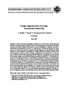
1.2 Motivation When we started our research, Color Image Segmentation had received much less attention than the gray-level counterpart from the scientific community, as stated in the very few surveys on the field [SKA94, LUC99, CHE01]. That was surprising because one intuitively feels that color is an important part of our visual experience, so it has to be useful or even necessary for powerful processing in computer vision [HUA92]. For instance, the human eye can only detect a few dozen intensity levels but can discern thousands of chromatic variations in a complex scene. Another fact that surprised us was that the majority of the proposed color segmentation algorithms were based on previous gray-level approaches adapted to the RGB or various HSI three-dimensional spaces. Conversely, we believe that color segmentation should deal with the perceptual meaning of the Hue-SaturationIntensity components. This idea is supported in some references [KEN76, TOM86, BAT93], which empirically proved that HSI channels carry information much more significant to humans than the RGB channels, especially on the Hue component. Other authors [OHT80, BER87, PER94] determined that Hue and Saturation are almost constant in front of illumination intensity variations. Therefore, our first motivation is the belief that separating the chromatic (Hue and Saturation) from the achromatic (Intensity) information can lead to robust color segmentation. Specifically, we expect that any segmentation based on H-S components will ignore light artifacts like shadowing and shadows on the objects. As a drawback, it will disable our algorithm to distinguish several intensities of the same dye. We guess that re-splitting the chromatic regions according to the Intensity component will remedy this situation. Figure 1.1 hypothetically illustrates this twostage segmentation on an example (Figure 1.1.a). The chromatic segmentation (Figure 1.1.b) shows one single color for each object of the scene. The achromatic refinement (Figure 1.1.c) splits each object into several areas, which are supposed to stand for different surfaces of the object. However, shadows may also be detected as “false” surfaces, but it is outside of our research scope. In spite of this, we think that this two-level segmentation may be very helpful in further image analysis steps.

18


a)

b)

c)

Figure 1.1 Segmentation example: a) input image; b) segmented regions according to their characteristic color; c) segmented regions according to their characteristic color and brightness.

The previous assumption is based on our conjectures about how the human being perceives colored objects. It cannot be formally proved because physiologists and biologists have not provided a general theory about this matter yet. Nevertheless, we must try some hypothesis in order to emulate the human segmentation skills through computer software. Besides the chromatic/achromatic dichotomy, we will also assume that humans perceive the scene as a hierarchical structure [MAR01]. It means that people can only recognize a few objects in a complex scene (typically the bigger ones). Eventually, they can recursively refine the description of an object or a smaller area of the scene, but with the same level of detail. Some computer-vision researchers point to 20 as the maximum number of objects that people can manage at a glance [LUO03]. Furthermore, we believe that humans associate a specific chromaticity to each object. Consequently, our second motivation is to develop a computerized system that can manage a set of relevant colors of the image, each color representing one relevant object of the scene. According to the previous reasoning, the segmentation system should not require more than 20 relevant colors. See Chapter 5 for a detailed explanation of these hypotheses. Finally, our third motivation is to find out a straightforward model for color data uncertainty. Specifically, we want to handle input signal noise, as well as illumination shading artifacts. Other uncertainty sources such as highlights, chromatic illumination or inter-reflection are so complex that they need specialized processes [KLI87, FIN98, BRI90]. For the shading artifacts, we have already proposed to consider

19

1 Introduction

chromatic and achromatic features separately, so the latter will isolate all the intensity variations. For the input signal noise, we will focus on the noise amplification due to non-linearity of the RGB-to-HSI transformation. Although there already exist such approaches [CAR94, BUR97, GEV01], we aim to establish a formulation able to predict the color data stability of any given pixel. This prediction will be included in our color-processing algorithms. Besides, the circular nature of the Hue component will also be taken into account, i.e. the Hue minimum and maximum values have a unitary distance. Very few researchers have included this characteristic in their proposals [TSE95, IKO00, ZHA00]. To cope with the proposed goals, we decided to implement labeled color image segmentation based on a set of relevant chromatic patterns. In order to find out, characterize and classify those patterns accounting for data vagueness, we chose to apply fuzzy techniques. Thus, we will take advantage of the extensive background of our research group in fuzzy theory and labeled image segmentation.

1.3 Objectives According to the aforementioned motivations, our general objective is: To carry out color image segmentation similarly to human beings, detecting a set of relevant chromatic patterns of the scene and then labeling the image pixels that belong to each pattern. Beyond the general objective, we have established other requirements that will be taken into account when designing the whole segmentation system: •

20

Illumination conditions. Both natural and artificial illumination sources will be allowed. Our system will only assume illumination intensity variations. Other artifacts such as highlight or chromatic illumination are supposed to be irrelevant.


•

Perceptual color. Our segmentation system will use the HSI components to describe color features: the Hue-Saturation pair will represent the chromaticity, while the Intensity component will stand for the brightness of the image pixels.

•

Data variability. We must assume a relative amount of noise in the input RGB channels. Thus, our system will account for the uneven H-S stability due to nonlinearity of the RGB-to-HSI conversion. The Hue circularity will also be taken into account in every difference calculation on the Hue values.

•

Achromatic feature. The Intensity component will only be considered after a primary H-S segmentation. In this way, we expect to provide initial object detection, and then provide surface detection within the objects based on the achromatic feature of their image pixels.

•

Autonomous behavior. We aim to develop methods that shall need a reduced degree of human intervention. At the same time, the results should be comparable to supervised segmentations, and should be obtained within a reasonable short period of time.

•

Robustness. Our system will be implemented using fuzzy techniques in order to provide resistance in front of the uncertainty sources of real scenes.

•

Usability. Although trying to segment any kind of scene is a very ambitious aim, our methods are intended to provide a low-level description of the image regions according to the previous ideas, so that the higher-level image analysis systems can reasonably interpret the segmentation results.

1.4 Thesis outline To cope with the stated objectives, we worked on two issues. Firstly, we performed an in-depth study of the HSI behavior in front of signal noise and illumination intensity variations. As a result, we have defined two Stability Functions, which can 21

1 Introduction

predict the reliability of the Hue and Saturation components of any color pixel. Secondly, we have designed a labeled color image segmentation scheme, which is structured into three main steps: Relevant Color Selection (including three alternative methods), Chromatic Pattern Characterization and Image Pixel Classification. Moreover, other extra steps can optionally perform achromatic re-segmentation and spurious region filtering, i.e. Fixed Gray-Level Characterization and Segmentation Refinements. The general workflow is depicted in Figure 1.2. Relevant Color Selection Automatic

Manual

Fixed

Chromatic Pattern Characterization Color Fuzzy Sets

Fixed Gray-Level Characterization Gray Fuzzy Sets

Image Pixel Classification

Segmentation Refinements

Original Image

Segmented Image

Figure 1.2 General scheme for our labeled color image segmentation.

22


The contents of this Ph.D. are organized in the following chapters: Chapter 2: Color Representation. This chapter provides a general background on the formation and representation of color information with electronic imagery systems. Chapter 3: State-of-the-art in Color Image Segmentation. The third chapter presents a survey on the existing methods for segmenting color images that are more or less related with our approach. Chapter 4: Stability of HSI components. In this chapter we explore the variability of the HSI color components in front of illumination intensity variations and signal noise. Consequently, we define the Hue and Saturation Stability Functions that will be included in all the proposed algorithms. Chapter 5: Automatic Detection of Image Relevant Colors. The fifth chapter describes our Automatic method for the Relevant Color Selection step. It constructs a fuzzy H-S histogram of the image, defined upon the stability of the input pixels. Afterwards, the method detects the relevant peaks of that histogram using our adaptation of the Watersheds algorithm. Each peak will be considered as a relevant chromatic pattern of the image, and will be passed to the next segmentation steps as two histograms, one for each chromatic component (Hue and Saturation). Chapter 6: Characterization and Classification of Chromatic Patterns. This chapter introduces our methods for the Chromatic Pattern Characterization and Image Pixel Classification steps. The first step obtains generic fuzzy sets from the chromatic pattern histograms, while the second step obtains a global membership degree for each pixel in each pattern. These processes account for the stability of the test data (input pixels) and the training data (pattern histograms). Moreover, the chromatic patterns tested in this chapter have been defined through the Manual method of the Relevant

23

1 Introduction

Color Selection step, i.e. obtaining their Hue and Saturation histograms from manually selected image pixels. Chapter 7: Additional Image Segmentation Steps. The seventh chapter introduces some extra methods aimed to complete our basic segmentation defined in the previous chapters. The Fixed method for the Relevant Color Selection step obtains a set of chromatic patterns from a global partitioning of the H-S space. The Segmentation Refinements step includes two optional processes. First, some filtering techniques make use of the neighboring pixel classification so as to get rid of spurious regions. Second, it performs the achromatic re-splitting of the chromatic regions, according to the Intensity of the input pixels and the generic achromatic fuzzy sets provided by the Fixed Gray-Level Characterization step (a fixed partitioning of the Intensity component). Chapter 8: Results. Once we have introduced our algorithms, this chapter presents a complete set of tests that empirically prove the validity of the proposed algorithms in front of a variety of images. The tests also compare our results with the results provided by some other methods. Moreover, the chapter presents a brief study of our system’s performance. Chapter 9: Conclusion. The final chapter plots the main contributions derived from our research, as well as several ideas for future work.

24


2 Color Representation To work in any field of Color Image Processing, one must first understand what color is and how it can be represented. This chapter is a brief introduction to the fundamentals of color information. Firstly, we present the general physics of color phenomena. The second section studies which stimuli are derived in the human eye and brain when we perceive colored light. The third section describes the basis of the colorimetric spaces defined by the CIE (Comission Internationale de l’Éclairage), which establish the standard references for industrial color management. The fourth section introduces the Red-Green-Blue (RGB) color coordinates provided by common image-capturing devices. Furthermore, some of the abundant color order systems derived from the RGB components are also presented. Specifically, we are interested in those transformations aimed to approximate the Hue-SaturationIntensity (HSI) perceptual components, i.e. the color information perceived by human beings. The final section sums up the main ideas exposed in the previous sections.

2.1 Physics of color 2.2 Human color perception 2.3 Colorimetric spaces 2.4 Color order systems 2.5 Summary

25

2 Color Representation

2.1 Physics of color Light is an energy flux composed by electromagnetic waves of diverse frequencies. Figure 2.1 depicts the whole range (spectrum) of the known electromagnetic waves, indexed by the logarithm of the wavelength λ. Human eye is only sensitive to a subset of wavelengths, so-called the Visible Spectrum [WYS82]. Radio TV Radar Microwaves 2

1

0

-1

-2

-3

-4

Infrared -5

log (λ (m))

-6

Ultraviolet

X-Rays

-7

-10

-8

-9

Gamma Rays

-11 -12

-13 -14 -15

Visible Light

10

700

600

500

λ (nm)

400

Figure 2.1 Electromagnetic spectrum and the Visible Spectrum.

Humans perceive each visible wavelength as a specific rainbow color (it excludes pinkish), but a full color sensation is actually determined by a composite of multiple light wavelengths: the spectral power distribution. Figure 2.2.a corresponds to the typical spectral power distribution of midday light, according to the CIE standards. Light Power (Watts)

1000

500

0.5

0.6 λ (µm)

0.7

500

0.0

0.8

0.4

b)

Reflected Radiance (Watts/m2·steradiant)

1000

0.5

0.4

a)

Object Reflectance (proportion)

1.0

0.5

0.6 λ (µm)

0.7

0.4

0.8

c)

0.5

0.6 λ (µm)

0.7

0.8

Figure 2.2 a) spectral power distribution of daylight (CIE standard Illuminant D65), b) reflectance of a green surface, c) spectral distribution of the reflected light.

When light “hits”! an object, the object surface absorbs the incoming energy per wavelength with different degree. This is known as the object reflectance, which is indeed a “spectral” distribution of absorbing degrees. Figure 2.2.b corresponds to an example of a green distribution. Figure 2.2.c represents the spectral distribution of the light returned (reflected) by the object, which corresponds to the multiplication of the

26


incident light distribution and the object reflectance distribution. In the example, the reflected distribution is more prominent in the central region of the visible spectrum. Therefore, the object appears to be greenish. The most generic formulation describing the geometry of the light reflection process is the Bi-directional Reflection Model [HOR86]. Figure 2.3 depicts the main geometric parameters, where dA is a differential of area of the observed surface, whose normal vector is aligned with the Z axis, dI is the irradiance of the illuminant beam, i.e. the light energy received on dA (Watts/square meter) from the incident direction (θi, φi), and dL is the radiance reflected by the surface, i.e. the light energy returned by dA through a differential of solid angle dωv (Watts/square meter · steradian) towards the viewing direction (θv , φv ). dI

Z

dL

dω i

dω v

θi

θv

φi dA

Y

φv

X

Figure 2.3 Representation of the Bi-directional Reflection Model.

To obtain the total radiance Lv (λ) received from a specific differential of area, we must integrate the radiance Li incoming through all possible directions of incidence. Equation 2.1 denotes this integration, where fr is the reflectance of the surface. Lv ( λ ) =

€

∫

ωi

Li (θ i , φ i , λ) f r (θ i , φ i ,θ v , φ v , λ )cosθ i dω i

(2.1)

The bi-directional reflection model is so complex that cannot be solved by actual computers. Many simplifications have been developed for Computer Graphics simulations. Equation 2.2 corresponds to the Phong’s approximation [PHO75], where Ea indicates the general ambient light energy and Ej is the light energy incoming from several light sources, θj is the angle of incidence of the incoming beams, φj is the

27


angle between the reflection direction and the viewing direction, Kd and Ks are the spectral distribution of diffuse and specular reflectance of the material, and n is a heuristic coefficient that indicates the roughness of the material (1 for very rough and 200 for very smooth). Lv ( λ ) = K d (λ ) E a ( λ) + ∑ E j ( λ )(K d ( λ)cos θ j + K s ( λ )cosn φ j )

(2.2)

j

€

Figure 2.4 represents the diffuse and specular reflection phenomena. The first one occurs when light enters into the material and is scattered by the colorant particles inside. Thus, part of this light comes back from the surface in all directions. On the contrary, specular reflection corresponds to the portion of incident light that is rejected by the object surface, which is mainly sent around the reflection direction (symmetric to the incident direction with respect to the surface normal N). specular direction

N

Ie θ

θ

Ii

specular spike

Id

medium

specular lobe

material

Ii diffuse lobe

material

colorant particles

a)

N

b)

Figure 2.4 Specular and diffuse reflection: a) light paths, b) reflected light distribution.

Equation 2.2 accounts for diffuse and specular reflection, but it ignores many aspects about real illumination, such as the shape and distance of the light sources, occlusions, and light emitted by nearby objects (inter-reflections). More complex models have been developed to simulate the physics of the reflection processes [FOL90, COO81]. Nevertheless, we are not interested in those light reflection models but in the colorimetric features of perceived light. Specifically, we generally expect that the diffuse reflection be determined by the intrinsic color of the object, while the specular reflection (highlights) returns the color of the incident light. Many researchers have based their image segmentation algorithms on these physics-related assumptions [SHA85, HEA87, HEA89, HEA91, TIA97].

28


2.2 Human color perception As denoted in the previous section, the full physical specification of a color stimulus is a function of the visible range of wavelengths. However, it is well known that the first stage of human color vision consists of three types of photoreceptor cells, socalled cones. There is a fourth type called rods, which is active at low light energy levels (nocturnal vision) but do not contribute to color vision [BOY79]. Each type of photoreceptor has specific spectral sensitivity, as shown in Figure 2.5:

Figure 2.5 Relative spectral sensitivity of the human photoreceptors (cones and rods).

Many papers name the cones as blue, green and red, but it is misleading because they have their maximum sensitivity at 437 (violet), 533 (green) and 564 (yellow) nanometers. It is more convenient to refer to them as short-, medium- and longwavelength photoreceptors. Equations 2.3 represent the neural excitation signal for each photoreceptor (CL, CM and CS) due to a generic color stimulus L(λ) filtered by each spectral sensitivity l(λ), m(λ), and s(λ) within the visible spectrum [λ1..λ2]: CL =

€

∫

λ2 λ1

L( λ ) l( λ ) dλ ; CM =

∫

λ2 λ1

L( λ ) m(λ ) dλ ; CS =

∫

λ2 λ1

L(λ ) s( λ) dλ

(2.3)

Coding the input color with three scalar values loses a great deal of spectral information, since two different spectral distributions may generate the same three neural signals. This phenomenon is known as metamerism. It means that biological color perception is actually quite restricted, but it is logically adapted to the minimum needs for the survival of the species. Many devices for representing color take advantage of this feature, thus needing only three or four basic dyes. For example, each pixel in a TV or computer screen can reproduce a wide range of colors by varying the relative amount of light emitted from three tinted phosphor elements. 29


It is generally accepted that the second stage of the visual system combines the primary signals provided by the cones as expressed in Equations 2.4, thus producing the opponent signals (the constants α, β and γ are conceptual and cannot be specified precisely): GR = α1CM − α 2CL ; BY = β1CS − β 2CM − β 3CL ; WB = γ1CS + γ 2CM + γ 3CL

€

(2.4)

The previous formulation models the reinforcement (addition) and inhibition (subtraction) of neural signals, which results in two chromatic signals contrasting the green against the red features (GR) and the blue against the yellow features (BY) of a color stimulus. There is also an achromatic channel (WB) that adds all primary signals to obtain brightness information (white against black). The Opponent-colors model is based on the theory of E. Hering, who pointed out (in the 19th-century) that neither the attributes of redness and greenness nor the attributes of yellowness and blueness could coexist in a perceived color. However, there is still no evidence that the neuralnetwork for generating the opponent channels exists [ROB92]. Our perception of color is not directly related with the cone signals or the opponent signals. Actually, human beings notice two basic types of spectral energy distributions, as represented in Figure 2.6. e2

E

e2

e1

e1

400

a)

E

500 600 λ (nm)

700

400

b)

500 600 λ (nm)

700

Figure 2.6 Basic types of spectral distribution perception: a) type 1; b) type 2.

Type 1 occurs when there is a peak of light energy emerging from the rest of the spectral distribution. In this case, we perceive the color associated to the peak wavelength (dominant wavelength). Type 2 occurs in the reverse situation, making us perceive the color inverse (opponent) to the one corresponding to the valley wavelength. In both cases, we perceive one single dye: red, green, yellow, blue,

30


orange, purple, pink, etc. We also perceive the purity of the color, according to ratio between the energy levels of the dominant wavelength and the rest of spectral distribution (if e1/e2=1, we perceive “gray”!). Moreover, we perceive global energy of a light signal (luminance). These variables are known as psychophysical stimuli [MAC35].

the the the the

The perception of color is not only determined by psychophysical factors but also by neighboring colors and other physiological and psychological factors. Ralph Evants suggested that there are five perceptual variables involved in color perception: Hue, Saturation, Lightness, Brightness and Brilliance [EVA74]. For non-fluorescent object colors, these variables can be reduced to the three former. According to A. Robertson [ROB92], «Hue is the attribute of a visual sensation according to which an area appears to be similar to one of the perceived colors red, yellow, green or blue or to a combination of two of them. Saturation is but one of several different terms, (…) the degree to which a perceived color differs from achromatic - white, gray or black. (…) Lightness is the attribute describing whether an object color appears lighter or darker than another under the same illuminating and viewing conditions.» Therefore, the perceptual variables hue, saturation and lightness are somehow related to the psychophysical variables dominant wavelength, purity and luminance, respectively. Faugueras [FAU79] defined an alternative triad of variables for coding human color perception considering the logarithmic sensitivity of the cone cells. The proposed codification includes one achromatic (A) and two chromatic (C1, C2) coordinates, as shown in Equations 2.5. The weighting factors of the achromatic variable correspond to the luminance perception of each photoreceptor, α = 0.612, β = 0.369, γ = 0.019. The other weighting factors (a, u1, u2) are specified in order to describe well the response of cells that really exist in the visual cortex. A = a(α logCL + β logCM + γ logCS ); C1 = u1 log(CL /CM ) ; C2 = u2 log(CL /CS )

€

(2.5)

From the above signals, Equations 2.6 define an ideal color space in conical coordinates, where L corresponds to the height (Lightness), C to the radius (Chroma), and H to the angle (Hue) of the color position within the color space: 31


L = A; C = C12 + C22 ; H = atan(C2 C1 )

€

(2.6)

Figure 2.7.a depicts the shape of the theoretical color space due to the above formulation. All colors with the same Hue lie on one radial plane. The Chroma is dependent on the Lightness value, thus provoking the inverse-cone shape of the space. We can detach these two coordinates by introducing the concept of Saturation as S = C/L. Therefore, the new shape of the solid is ideally a cylinder (Figure 2.7.b). A

A Chroma

Lightness

Lightness

C2

C2

C1

Hue

a)

C1

Hue

Saturation

b)

Figure 2.7 Perceptual color space based on (A, C1 , C2 ): a) conical; b) cylindrical.

The cylindrical space is more convenient for color representation purposes, since their coordinates are highly independent. However, we must be aware that the maximum vivid colors observable in reality (optimal colors [POI80]) define very irregular limits of the color space. Moreover, Hue is undefined for achromatic colors (S = 0), and Saturation is undefined for the absolute black (L = 0). Nevertheless, perceptually organized color spaces allow designing computer applications able to manage color information in the way human beings do.

2.3 Colorimetric spaces In 1931 the CIE (Comission Internaltionale de l’Éclairage) established the colorimetric principles that had been adopted by industry as the standard color reference system. The classical book that lays down the CIE color spaces is the one written by Wyszecki and Stiles [WYS82]. For a critical review of the CIE color fundamentals examined from the latest knowledge, see [FAI97].

32


The CIE system is based on Grassmans’ experiments performed (in 1853) with colorimeters. A colorimeter projects a test light onto a half of a white surface. The other half (separated by a black partition) is illuminated with three primary lights. A person can vary the intensity of the three primaries in order to equal (match) the perceived color on both sides of the viewed surface (Figure 2.8). The primaries must have independent spectra, but no other special specification. Primary lights Reduction screen and sorround

White surface with Black partition Test light

Figure 2.8 A colorimeter for matching the test light with three primary lights.

Equation 2.7 expresses Grassmans’ law, where Q(λ) is the spectral power distribution to be matched, P1(λ), P2(λ), P3(λ) are the spectral power distribution of the primary lights, and a, b, c are the intensity coefficients of the primaries. The colorimetric equality =ˆ stands for a metameric match, so the resultant spectral power distribution at each side of the expression might be different. Q( λ ) =ˆ aP1 (€ λ ) + bP2 ( λ) + cP3 ( λ )

€

The addition of the three primaries cannot sometimes provide the full saturation of certain test lights. This situation can be overcome by adding one or two primaries to the test light, which leads to negative values of the coefficients (Equation 2.8): Q( λ ) + aP1 (λ ) =ˆ bP2 ( λ) + cP3 ( λ ) ⇒ Q(λ ) =ˆ −aP1 (λ )bP2 (λ ) + cP3 ( λ )

€

(2.7)

(2.8)

If test and primary lights are monochromatic and if there exists a wide range of wavelengths for the test lights, then we can compute the approximate coefficients of the primaries for the visible spectrum. This procedure was carried out on a group of

33


testing people, so the average of the obtained coefficients were accepted as the 1931CIE Color-Matching functions (Figure 2.9). 3.0 2.5

r(λ) 2.0 1.5

b (λ )

1.0

g (λ )

0.5 0.0 -0.5

390 430 470 510 550 590 630 670 710 (nm)

Figure 2.9 The 1931-CIE RGB color-matching functions.

Equations 2.9 define the three coefficients R, G and B to match any polychromatic stimulus Q(λ). Actually, the real calculations consist in summing-up the energy values of Q multiplied by the color-matching values at many discrete wavelengths. R=

€

∫

λ2 λ1

Q( λ ) r (λ ) dλ ; G =

∫

λ2 λ1

Q(λ ) g ( λ) dλ ; B =

∫

λ2 λ1

Q( λ)b ( λ ) dλ

(2.9)

Equation 2.10 describes the polychromatic stimulus Q(λ) as the colorimetric proportion of the primary spectral distributions R(λ), G(λ) and B(λ), according to the coefficients obtained in Equations 2.9. Q( λ ) =ˆ RR( λ) + GG(λ ) + BB( λ )

€

(2.10)

The 1931-CIE RGB space is able to represent any color reliably, but it also has some drawbacks. One of the most evident is that the Red color-matching function presents some negative values. To solve some of the inconvenience, the CIE approved the convention of three new reference primaries, which were called XYZ. Those primaries didn’t have to correspond to any physical color, but they were carefully chosen to have all-positive color-matching functions. Besides, other requirements were considered, such as to obtain equal coordinates for the achromatic stimuli and to make one of the components (Y) corresponding with the luminance of any stimuli.

34


The conversion between RGB to XYZ coordinates is linear, and can be done by the matrix-vector multiplication expressed in Equation 2.11:  X   0.490 0.310 0.200  R         Y  =  0.177 0.812 0.011 ⋅ G        Z   0.02 1.071 0.408  B 

€

(2.11)

Figures 2.10 illustrate the three-dimensional relationship between the RGB space and the XYZ space. Figure 2.10.a represents the solid defined by all possible color stimuli within the RGB space. The perpendicular cut shows all colors with the same luminance. The horseshoe-shaped border contains all monochromatic light, which is called the spectrum locus. The line connecting the ends of the spectrum locus is known as the purple boundary. Any polychromatic light Q always lies within the limits of the spectrum locus and the purple boundary, and it can be expressed as a linear combination of the three primary vectors R, G and B. Y

G

y Y

Q

x R

Z

a)

B

b)

Z

X

X

c)

Figure 2.10 Three-dimensional representation of two color spaces: a) the RGB space; b) the XYZ space; c) the XYZ projection onto the x-y chromaticity plane.

The positive values of the RGB components can only generate the colors enclosed within the triangle connecting the three primaries. Thus, the XYZ space was defined to contain all possible colors within the positive part of their axis (Figure 2.10.b). If we normalize the XYZ coordinates as expressed in Equations 2.12, one of the new coordinates xyz is redundant (e.g. z). Geometrically, it corresponds to a projection of the cut plane X+Y+Z=1 onto the 2D chromaticity plane (Figure 2.10.c). x=

€

X Y ; y= ; z = 1− x − y X +Y + Z X +Y + Z

(2.12)

35


Psychophysical color can then be specified as (Y, x, y), since Y represents the lightness and x-y represents the chromaticity of the stimulus. Thus, Figure 2.11 represents all possible chromatic values, i.e. the chromaticity diagram. x 0.2 520

0.4

0.6

0.8

530

1.0 0.8

540

510

550

A

560

0.6 570

500

D E 490

y

580 590 600 C 630660 700

0.4

0.2 480

B

470 430 380

0.0

Figure 2.11 The 1931-CIE x-y chromaticity diagram.

The central point E represents the achromatic stimuli (x=y=z=1/3). A line connecting the central point with any border point D contains all possible saturations of the dominant wavelength of D. A positive combination of three colors A, B and C render any of the colors inside the ABC triangle (e.g. the color palette of a TV set). The original color-matching functions were reviewed in 1964 to adjust the response of real observers. Despite the improvements, the 1964-CIE Yxy color space still lacks one important characteristic. Namely, the geometric distance between two points does not correspond with the perceived differences between the corresponding colors. In order to correct this, in 1974 the CIE proposed the L*u*v* space (also known as U*V*W*) and the L*a*b* space (usually noted as LAB). The latter is defined by Equations 2.13, where (X0, Y0, Z0) are the XYZ coordinates of a white reference and f(x) is a function defined in Equation 2.14. L* = 116 f (Y Y0 ) −16 ; a* = 500[ f (X X 0 ) − f (Y Y0 )] ; b* = 200[ f (Y Y0 ) − f (Z Z 0 )]

€

€

3 x ; if x > 0.008856 f (x) =   7.787x + 16 /116 ; otherwise

36

(2.13)

(2.14)


Figure 2.12 shows two views of the L*a*b* solid limited by the optimal colors, i.e. the maximum saturation that can be found in nature [POI80].

a)

b)

Figure 2.12 The optimal 1976-CIE LAB space: a) side view; b) top view [HIL97].

The LUV and LAB spaces are intended for estimating the human perceived difference between two colors as their Euclidean distance within the space. However, they are not perfect perceptually uniform color spaces, as some researchers claim. An alternative color difference calculation was introduced by CIE in 1994 in order to obtain constant perceptual differences for every pair of colors, but it is only a tolerance formulation based on LAB coordinates [ALM93].

2.4 Color order systems The CIE standards were designed to reproduce color on industrial goods in a very precise way. We must know these standards because they are frequently referred in the literature. Nevertheless, only spectrometers (multi-band image capturing devices) can deal with accurate color coordinates. The CCD cameras or scanners used for Computer Vision applications cannot provide reliable XYZ or LAB coordinates. On the contrary, the typical output of CCD devices is the Red-Green-Blue (RGB) coordinates, which are not related by any way with the CIE RGB coordinates or the human photoreceptor signals. In the present section, we first explain the particularities of the CCD RGB color system. Then, we present several mathematical formulations for deriving other color

37


coordinates from the RGB ones, in order to enhance specific features of color information. Specifically, we are very interested in characterizing some sort of HueSaturation-Intensity (HSI) features, thus representing somehow the human perceptual attributes. 2.4.1 The RGB color system Typical CCD color cameras provide three values for every image pixel. Each value corresponds to the light energy gathered by one of three channels Red, Green and Blue. Those channels are determined by color filters having a particular spectral response r’(λ), g’(λ) and b’(λ). The RGB values for each pixel are determined by Equations 2.15, where L(λ) is the power spectral distribution of the input light and [λ1.. λ2] is the integrating wavelength range [LUO91]. R=

€

∫

λ2 λ1

L( λ )r'( λ )dλ ; G =

∫

λ2 λ1

L( λ )g'( λ )dλ ; B =

∫

λ2 λ1

L( λ )b'( λ )dλ

(2.15)

This formulation is similar to the human photoreceptors (the cones) but their spectral responses do not € coincide with the camera € filters. Besides, the filter responses do not has any similarity with the CIE RGB color matching functions either. Consequently, the RGB coordinates obtained with a CCD camera cannot be considered as standard values of the captured colors. It must also be remarked that RGB coordinates can only represent colors within the gamut defined by the spectral response of their channel filters. The full color gamut of the physical world always exceeds the RGB gamut. Hence, some extreme colors get mapped into a “wrong” RGB triplet [HIL97]. This is why the RGB color system should not be referred as a chromatic space but as a color order system. Nevertheless, it is very common to use the term color space instead of color order system space for compactness reasons. There are other features of the camera and the digitizer (the device for converting analogical video into digital numbers) that may alter the RGB values:

38


• The sensitivity of the CCD sensors is logarithmic. Some cameras or digitizers implement a gamma correction mechanism in order to provide a linear response to the input light energy of each channel. • Auto-exposure systems automatically adjust the shutter speed or the diaphragm aperture of the camera to make sure that the average light intensity of the scene falls within an appropriate range for the sensors. • The density of each color filter differs from one to another, so the achromatic light produces different values in each RGB channel. To overcome this problem, many cameras implement a sort of channel calibration mechanism called white-balance, which equalizes the channel responses for a given white reference. One might try to calibrate the camera to achieve reliable RGB values in front of variations of the illumination. For example, Y.C. Chang et al. [CHA96] proposed a method based on a reference color chart placed in the field of view of the camera. Comparing the sampled RGB values with the real RGB values of the chart, we can derive an inverse transform to obtain the original RGB color values of the whole image. More sophisticated and generic calibration procedures can be applied through the definition of the camera profile (for instance, an ICC profile), which can extrapolate the RGB values into the CIE XYZ or LAB spaces. In this way, we can obtain standard color coordinates for transmitting the image pixels to any color reproduction system, approximately preserving their original chromaticity. On the contrary, the habitual situation for Computer Vision systems is to use the raw RGB values provided by non-calibrated color cameras under unknown illumination conditions. This is logical because the Computer Vision purpose is to detect and recognize objects, usually according to pixel differences or similarities. Thus, when processing color images it is not important to obtain the exact color reference of the objects, because it is supposed that color differences or similarities will be more or less unaffected by RGB distortions.

39


Figure 2.13.a represents the limits of the RGB color order space, known as the RGB cube. Figures 2.13.b and 2.13.c show two perspective views of the cut planes for equal light lightness in the three coordinates (R+G+B = constant). G G

G

R B

R

B

R

B

a)

b)

c)

Figure 2.13 The RGB cube: a) volume; b,c) planes with R+G+B = constant.

The range of RGB coordinates can be specified as a real number between 0.0 and 1.0, or as a natural number between 0 and the maximum value obtained with the number of bits used in the coordinate quantization. For example, MAX_RGB = 255 for 8 bits per channel (24 bits color representation). 2.4.2 The I1-I2-I3 color system A great many of color transformation formulae have been proposed in order to convert the basic RGB coordinates into others which might be more convenient for certain applications. For example, Ohta et al. [OHT80] defined the I1-I2-I3 color coordinates by means of a Karhunen-Loewe analysis of some RGB color samples extracted from eight natural images. This method obtains statistically uncorrelated coordinates, i.e. I1 is the optimal base vector gathering the maximal variance, I2 is an orthogonal vector that best gathers the remaining variance, and so on. Equations 2.16 express the RGB linear transformation for each coordinate: I1 = (R + G + B) /3 ; I2 = (R − B) /2 ; I3 = (2G − R − B) /4

€

(2.16)

The authors claimed that this transformation is the most suitable for detecting color differences, €but one can argue € that it is only true for the concrete images used to obtain the eigenvectors.

40


Figure 2.14.a shows the shape of the I1-I2-I3 color order space. Notice that the I1 component corresponds to the main diagonal of the RGB cube. Hence, diagonal cut planes correspond to horizontal planes in the new color space (see Figure 2.14.b). I1

I1

I3

I3

I2

a)

I2

b)

Figure 2.14 The I1-I2-I3 color system: a) volume; b) planes with R+G+B = constant.

2.4.3 Computational HSI color system Many linear RGB transformations proposed in the literature correspond to a rotated and scaled cube like in the I1-I2-I3 system, for example, the YIQ system for TV color signals. In most cases, one of the axes stands for the Intensity value of the color, while the other two may be interpreted as the chromaticity values. However, if we need to represent the human color perception, we should use one of the available transformations to convert RGB into HSI components. Figure 2.15 depicts how to r interpret the HSI components of a color point (or vector) c within the RGB cube. Green

c

€

s h i

Red Blue

Figure 2.15 Hue-Saturation-Intensity definition (h, s, i) within the RGB color cube.

In the previous graphic, the Intensity component is the distance between the origin of the cube (R=G=B= 0) and the diagonal cut plane (R+G+B= constant) containing the

41


r color point c . The Saturation component is the distance between the center of the r cut plane (the achromatic point, R=G=B= constant) and the color point c . The Hue component is the angle between the saturation vector and the Red reference vector € contained within the cut plane (by convention, H = 0º for pure red). One can find € many definitions of the HSI components in classical Computer Vision books [PRA78, GON92]. Besides, different notations are used for the Intensity component (Value, Lightness, Brightness), but we always use HSI to unify the perceptual color names. 2.4.4 The Tenenbaum’s HSI color system Tenenbaum et al. [TEN74] defined the RGB-to-HSI non-linear transformation depicted in Equations 2.17. The H component is provided within the [0..2π] range, so the appropriate scaling must be applied in order to normalize it with the range of the other two components.  3(G − B)  Min(R,G,B) H = arctan ; I = (R + G + B) /3  ; S = 1− (R + G + B) /3  2R − G − B 

€

(2.17)

Figure 2.16.a shows the outline of the Tenenbaum’s HSI space. This color space is a € cylindrical volume € bounded by different Intensity maximums for each Hue-Saturation pair. Figure 2.16.b shows several constant lightness planes, which are horizontal, i.e. independent from the other two components. I

I

S

a)

H

S

b)

H

Figure 2.16 The Tenenbaum’s HSI system: a) volume; b) planes with R+G+B = constant.

42


2.4.5 The Smith’s HSI color system If we need a HSI space with straight limits, we can use the Smith’s transformation [SMI78]. First, the RGB components are scaled within their maximum and minimum values, thus obtaining normalized rgb components (Equations 2.18). Then, Hue is obtained with the two of the rgb components as expressed in Equations 2.19. This transformation obtains a Hue value between [-1/6..5/6]. We can correct the negative part of the range by adding 1 to the negative values, thus obtaining the range [0..1] (since Hue is an angle, it is modular). r=

€

€

(2.18)

 (b − g) /6, if (R = maxRGB )    H = (2 + r − b) /6, if (G = maxRGB ) ; if (H < 0) then H = H + 1.0 € € (4 + g − r) /6, if (B = maxRGB ) S=

€

max RGB − R max RGB − G max RGB − B ; g= ; b= maxRGB − minRGB maxRGB − minRGB maxRGB − minRGB

(2.19)

maxRGB − minRGB € RGB ; I = max max RGB

(2.20)

The Intensity and Saturation components expressed in Equations 2.20 define the € cylindrical shape of the color space, as can be seen in Figure 2.17.a. Therefore, we obtain independent HIS components, which is a highly desirable property for any color space. I

I

S

a)

H

S

b)

H

Figure 2.17 The Smith’s HSI color system: a) volume; b) planes with R+G+B = constant.

43


However, we must be aware that equalizing the maximum Intensity value for all H-S pairs is misleading. For example, Red, Green and Blue dyes are darker than Yellow, Cyan and Magenta dyes. It can be observed in Figure 2.17.b, where the planes corresponding to colors with constant lightness become very irregular surfaces within the HSI cylinder. Besides, the S component is unevenly equalized, because darker (bottom) areas have less number of colors than brighter (top) areas. For example, when I = 0 (R=G=B= 0) there is no Saturation (one must avoid the S calculation). Another singularity is produced at S = 0 (R=G=B= constant), where the Hue is undefined because it corresponds to the achromatic (gray) colors. These artifacts lead to a non-linear color distribution of the Smith’s HSI volume, meaning that low color-density areas are more sensitive to RGB variations than high color-density areas. Hence, the RGB input noise gets annoyingly amplified in the conflictive parts of the HSI space. 2.4.6 The Yagis’s HSI color systems For uniform color density spaces, one might use the Yagi-Abe-Nakatani [YAG92] HSI models. These authors proposed two variants of the Saturation and Intensity components, while keeping the same Hue component of the Smith’s model. The first variant is obtained through Equations 2.21, and depicted in Figure 2.18. S = maxRGB − minRGB ; I =

maxRGB + minRGB 2

(2.21)

I

€

I

€

S

a)

H

S

b)

H

Figure 2.18 First Yagi’s HSI color system: a) volume; b) planes with R+G+B = constant.

44


The double cone shape accounts better for the limits of the RGB color system, because there are fewer colors for very dark or very bright zones of the RGB cube. The cut planes for constant lightness (Figure 2.18.b) still become irregular surfaces for this model, but with less distortion than the Smith’s model. The second variant of the Yagi’s model proposes to use the arithmetic mean of the RGB values for obtaining the Intensity component (Equations 2.22). The resulting volume and constant lightness cut planes are depicted in Figure 2.19. Now the cut planes are horizontal, but the saturation limits are not circular: the double cone becomes a rounded rotated cube. S = maxRGB − minRGB ; I =

€

R+G+ B 3

(2.22)

I

I

€

S

S

a)

H

b)

H

Figure 2.19 Second Yagi’s HSI color system: a) volume; b) planes with R+G+B = constant.

It seams impossible to define a HSI space based on RGB coordinates, which offer an orthogonal shape and horizontal cut planes for equal lightness at the same time. Nevertheless, we have obtained very good results using the Smith’s model because of the independence between its components. The drawbacks of this model can be reasonably assumed by taking into account the non-uniform density of the color volume (see Chapter 4).

45


2.5 Summary The work developed in Chapter 2 can be summarized as follows: •

Physical color is very complex. The exact spectral power distribution reflected by an object depends on a huge amount of variables, i.e. illumination features, object reflectance, incident and viewing directions, etc.

•

Human color perception can be defined with three parameters. The human eye is sensitive to three wide bands of the visible spectrum. The human brain interprets these primary signals into three other perceptual signals, which make us describe color in terms of hue, saturation and intensity.

•

Industrial color management systems are also based on three parameters. Taking advantage of the human vision physiology, the CIE standard spaces can precisely manage color with just three coordinates.

•

RGB cameras cannot provide exact color coordinates. The typical RGB cameras based on CCD technology can only provide a distorted subset of chromaticity of the real world.

•

Computational HSI spaces approximate human color perception. Through mathematical formulation, it is possible to convert original RGB components into HSI components, which are intended to emulate the perceptual variables involved in color perception.

As a conclusion, we propose that Computer Vision algorithms aimed to deal with color images should work with computational perceptual variables, despite of the uneven color density of these perceptual spaces. Our experiments have shown that any algorithm based on some sort of HSI components, and specifically on the Smith’s formulation, will succeed in identifying the main chromaticity of the scene objects (see Chapter 8).

46


3 State-of-the-art in Color Image Segmentation Before designing our color segmentation algorithms, we must first look into the bibliography for existing approaches in order to understand the related problems and improve the actual results. This chapter summarizes a range of proposals for segmenting images into regions of homogeneous color. The first section introduces the classification criteria of the collected papers. The second and third sections depict the feature-based approaches, i.e. Histogram thresholding and Clustering techniques, which look for agglomerations of pixels (histogram peaks or clusters) within the feature (color) space. These agglomerations are considered as color classes. Therefore, the segmentation problem can be understood as a classification problem: each pixel is assigned to one color class. The fourth and fifth sections depict the image-based approaches, i.e. Edge or Region detection techniques, which evaluate the color dissimilarity or similarity of neighboring pixels within the image space. Hence, grouping or splitting spatially connected sets of pixels determines image regions. The final section renders the particular advantages and drawbacks of each group of proposals.

3.1 Introduction 3.2 Histogram thresholding techniques 3.3 Clustering techniques 3.4 Edge detection techniques 3.5 Region detection techniques 3.6 Summary

47

3 State-of-the-art in Color Image Segmentation

3.1 Introduction For each paper described in the next sections, we present the following fields: Title: Authors: Ref.: Dim.: Space: Circ.: Preprocess: Method: Post-process:

title of the paper list of the authors Reference code (three letters of the first author and publication year) code of data dimensionality (see explanation below) color coordinates used in the proposed method indicates if the method accounts for Hue circularity brief description of preprocessing of the input data brief description of the main strategy brief description of post-processing of the output data

The dimensionality code expresses the number of color coordinates simultaneously used by the method (1D, 2D or 3D). If color coordinates are used independently for a later combination of their result, we express it as the number of coordinates multiplied by the single dimensionality (for example, 3 x 1D). If the method performs segmentation based on the analysis of one set of color coordinates within the regions obtained from previous segmentation of another set of color coordinates, we express it as a sequence of dimensionalities separated by semicolons (for example, 1D; 1D). If the method is intended for various dimensionalities, we show them separated by slashes (for example, 2D / 3D). In each section, the papers are sorted according to the year of publication (visible in the reference code). Some papers are difficult to classify in one of the following sections because they use various techniques. In this case, we have included them into the group corresponding to its principal segmentation strategy.

48


3.2 Histogram thresholding techniques Histogram thresholding is among the most popular techniques for segmenting graylevel images [SAH88]. It consists in delimiting the significant peaks in the image histogram, which gathers the relevant agglomerations of input pixels. Each peak can be considered as a class in the color space. Since these classes usually overlap, thresholds between peaks have to be fixed properly at histogram valleys. Color segmentation methods may process the histograms of each color coordinate individually, or may process a comprehensive histogram of the 2D or 3D color space (see the dimensionality code). Once the color space is tessellated with the proper thresholds, each pixel is classified into the color partition (class) that encloses the pixel coordinates. Thereafter, the groups of pixels that belong to the same color class and are connected in the image space can be considered as the segmented regions. Typically, color classes obtained with this technique are quite insensitive to input noise, due to the great many of pixels that build each histogram peaks. However, the segmented regions are rather jagged and with many spurious areas inside, because the pixel classification process does not take into account the image-space coherence of the regions. Hence, filtering post-processing is usually applied. Furthermore, the color distribution of small areas of the image may be occluded by other bigger distributions within the histogram. Besides, the thresholds on the Hue coordinate must be aware of the circularity of this component, i.e. the color partitions may cross the Hue limits. Title: Picture segmentation using a recursive region splitting method Authors: R. Ohlander, K. Price, R. D. Ray Ref.: [OHL78] Dim.: 9 x 1D Space: RGB, HSI, YIQ Circ.: No Method: Select best peak of the nine histograms, and recursively split regions of connected pixels falling in the most populated peak interval.

Title: Authors:

Color Information for Region Segmentation Y. Ohta, T. Kanade, T. Sakai

49


Ref.: [OHT80] Dim.: 3 x 1D Space: I1-I2-I3 Circ.: --Preprocess: Established the new I1-I2-I3 color space, based on a KL transform of the RGB values.

Method:

Same as in [OHL78], but using the new coordinates.

Title:

Opponent colors as a 2-dimensional feature within a model of the first stages of the human visual system

Authors: K. Holla Ref.: [HOL82] Dim.: 2D Space: Opponent Preprocess: Pass-band filtering. Method: 2D thresholding of the RG-YB histogram.

Circ.: ---

Title: Color image segmentation using three perceptual attributes Authors: S. Tominaga Ref.: [TOM86] Dim.: 3 x 1D Space: HSV, Munsell Circ.: No Method: Same as in [OHL78], but with a KL transform of the HSV and Munsell coordinates.

Title:

A color classification method for color images using a uniform color space

Authors: S. Tominaga Ref.: [TOM90] Dim.: 3 x 1D Space: Lab Circ.: --Method: Same as in [OHL78], but with a KL transform of the Lab coordinates. Post-process: Merge clusters that are too near. Title:

On the color image segmentation algorithm based on the thresholding and the fuzzy C-means techniques

Authors: Y.W. Lim and A.U. Lee Ref.: [LIM90] Dim.: 3 x 1D Space: RGB, XYZ, YIQ, UVW, I1 I2 I3 Circ.: --Method: Find relevant valley positions in each coordinate through Scale-Space Filtering (SSF) and validate 3D clusters according to the number of pixels.

Post-process: Fuzzy C-mean distance to the cluster centers.

50


Title: A color clustering technique for image segmentation Authors: M. Celenk Ref.: [CEL90] Dim.: 1D Space: Lab Circ.: --Method: General thresholding on 1D Fischer transform of the Lab coordinates. Title: Color image segmentation using modified HSI system for road following Authors: X. Lin, S. Chen Ref.: [LIN91] Dim.: 1D Space: HSI Circ.: --Method: Bimodal thresholding on an empirical function (road / non-road) based on Saturation and Intensity components.

Title: Authors: Ref.: [TSE95] Preprocess: Method:

Circular histogram thresholding for color image segmentation D.C. Tseng, Y.F. Li, C.T. Tung

Dim.: 1D

Space: HSI

Circ.: Yes

Optimal SSF filtering based on entropy (not circular). Find best threshold on the Hue histogram and interchange sub-regions (circularity); recursive bi-section based on the maximum variance.

Title: An algorithm for unsupervised color image segmentation Authors: L. Lucchese, S.K. Mitra Ref.: [LUC98] Dim.: 1D; 1D Space: Yuv Circ.: No Preprocess: Color quantization and wavelet low-low band filtering. Method: Hue(u,v) histogram thresholding and second histogram thresholding on Saturation(u,v).

Post-process: Image median filtering. Title: Authors: Ref.: [SHA98] Preprocess: Method:

Histogram-based segmentation in a perceptually uniform color space L. Shafarenko, M. Petrou, J. Kittler

Dim.: 2D / 3D

Space: Luv

Circ.: No

Adaptive Gaussian filtering of the Luv histogram. Watershed thresholding of the u-v or the Luv histograms.

51


Title: A new technique for color image segmentation Authors: C. Amoroso, E. Ardizzone, V. Morreale, P. Storniolo Ref.: [AMO99] Dim.: 1D Space: HSI Circ.: Yes Preprocess: Image filtering with a circular weight median and Hue histogram smoothing with Gaussian filters.

Method:

Hue Histogram valley detection with zero crossing of a functional (circular convolution).

Post-process: Neural network trained for color class recognition. Title:

Segmentation of digitized dermatoscopic images by two-dimensional color clustering

Authors: P. Schmid Ref.: [SCH99] Dim.: 2D Space: Luv Circ.: --Preprocess: Image median filtering and histogram Gaussian filtering. Method: Contour line analysis on 2D histogram of the KL transformed Luv space, applying directional Fuzzy C-means.

Post-process: Morphological filtering of the segmented regions. Title: A hierarchical approach to color image segmentation using homogeneity Authors: H.D. Cheng, Y. Sun Ref.: [CHE00] Dim.: 1D; 1D Space: HSI, Lab Circ.: No Preprocess: Obtain the homogeneity histogram on Intensity. Method: Split image according to Intensity thresholds and then apply a second thresholding on the Hue histogram of the initial regions.

Post-process: Region merging in image space if Lab distance is low. Title: Authors: Ref.: [GER01] Preprocess: Method:

52

Color image segmentation based on automatic morphological clustering T. Geraud, P.Y. Strub, J. Darbon

Dim.: 3D

Space: RGB

Gaussian and morphological filtering of the 3D histogram. Connected watershed thresholding of the RGB clusters.

Circ.: ---


Post-process: Markovian labeling of the output image. Title:

Detection of grey regions in color images: application

to

the

segmentation of a surgical instrument in robotized laparoscopy

Authors: C. Doignon, F. Nageotte, M. De Mathelin Ref.: [DOI04] Dim.: 1D Space: HSI (Saturation only) Circ.: --Preprocess: Sigma filtering of the Saturation component; Gaussian filtering of the Saturation histogram.

Method: Recursive histogram thresholding to locate significant Saturation minima. Post-process: Region growing from low-saturated pixels; edge detection on the obtained regions, in order to find a metallic surgical instrument.

3.3 Clustering techniques Histogram thresholding can be considered as a sort of clustering technique because it defines the boundaries (thresholds) of the classes or clusters within the feature space. However, the classical clustering method concerns the problem of determining the proper center of the clusters, and typically classifies each test sample not depending on its position relative to the cluster boundaries but on a distance calculation relative to the cluster centers. Consequently, there is no need to obtain the cluster boundaries to proceed with the classification, but distance calculus on the Hue coordinate must account for circularity. Moreover, the computation of cluster centers usually involves all image pixels as individuals, thus neglecting the coincidence of many pixels into the same position of the feature space. This leads to one of the main drawbacks of clustering techniques: the huge computational effort required for dealing with all pixels as the training set. There exist some strategies to reduce the cardinality of the training set. Nevertheless, clustering usually needs iterative or recursive procedures to reach optimal solutions. Another important drawback is that most clustering methods need some sort of initialization provided by a human operator, the most common of which is the total

53


number of clusters (colors) appearing in the scene. Hence, there are very few unsupervised strategies in the bibliography. Finally, clustering-based results also present a lack of spatial coherence similar to histogram-based results. Title: Authors: Ref.: [SAR81] Preprocess: Method:

Segmentation of chromatic images A. Sarabi, J.K. Aggarwal

Dim.: 3D

Space: XYI

Circ.: ---

Input the initial number of clusters. Sequentially extract cluster centers and near bins from a binary-tree histogram.

Post-process: Manually refine the clustering of the unclassified bins. Title: Iterative fuzzy image segmentation Authors: T.L. Huntsberger, C.L. Jacobs, R.L. Cannon Ref.: [HUN85] Dim.: 3 x 1D Space: RGB, I1-I2-I3 Circ.: --Method: Iterative Fuzzy C-means on some randomly chosen input pixels, and labeling through α-cut.

Post-process: Join closer clusters. Title: Authors: Ref.: [TRI86] Preprocess: Method:

Low level segmentation of aerial image with fuzzy clustering M.M. Trivedi, J.C. Bezdek

Dim.: n x 1D

Space: Multi-band

Circ.: ---

Obtains PDS (Pyramid Data Structure) of each image channel. FCM (Fuzzy C-means) from low to high resolutions, splitting non-reliable pixels into the next FCM stage.

Post-process: Combine channel segmentation results. Title:

Pyramid segmentation of color images using fuzzy C-means clustering algorithm

Authors: J. Liu, W. Xie Ref.: [LIU93] Dim.: 3 x 1D Space: RGB Circ.: --Preprocess: Obtains PDS (Pyramid Data Structure) of each image channel. 54


Method:

Same as in [TRI86], but weighting the cluster center distance by the number of classified pixels in each cluster.

Post-process: Combine channel segmentation results. Title:

Automatic colour segmentation algorithms with application to skin tumor feature identification

Authors: S.E. Umbaugh, R.H. Moss, W.V. Stoecker, G.A. Hance Ref.: [UMB93] Dim.: 3D Space: RGB, HSI, Luv Circ.: No Preprocess: Input the number of clusters. Method: Similar to [OHT80], but splitting the feature space by the median color of the image region to be segmented.

Post-process: Classify pixels to the nearest cluster center. Title: Color image segmentation using a possibilistic approach Authors: K.B. Eum, J. Lee, A.N. Venetsanopoulos Ref.: [EUM96] Dim.: 3D Space: RGB, XYZ, I1-I2-I3 Circ.: --Preprocess: Input the initial number of clusters. Method: Possibilistic C-means clustering and selection of best-classified pixels as region seeds.

Post-process: Region growing from the obtained seeds. Title: Fuzzy clustering for color recognition application to image understanding Authors: L. Khodja, L. Foulloy, E. Benoit Ref.: [KHO96] Dim.: 2D Space: Yc1 c2 Circ.: --Preprocess: Input training color samples. Method: Triangulation of the training pixel positions within the feature space defines the shape of fuzzy membership functions of color classes.

Title:

Adaptive color segmentation: a comparison of neural and statistical methods

Authors: E. Littman, H. Ritter Ref.: [LIT97] Dim.: 3D

Space: RGB, Yuv, YQQ

Circ.: ---

55


Preprocess: Method:

Input training pixels. LLM (Local Linear Maps) Neural Network trained to distinguish hand and background.

Post-process: Compare with an adaptive Bayesian method. Title: Color Image Segmentation Using Hopfield Networks Authors: P. Campadelli, D. Medici, R. Schettini Ref.: [CAM97] Dim.: 3 x 1D Space: RGB, I1-I2-I3 Circ.: --Preprocess: SSF (Scale-Space Filter) to obtain the number of clusters and initialize the cluster centers.

Method:

Hopfield neural network with MxNxS neurons (MxN= image size, S= number of clusters).

Post-process: Combine channel segmentation results. Title: Unsupervised segmentation of color images Authors: G. Guodong, S. Yu, S. Ma Ref.: [GUO98] Dim.: 3D Space: Luv Circ.: --Preprocess: Threshold the mode / valley cells based on entropy. Method: Obtain the final number of clusters and its representatives (mean vectors) through a modified version of the Akike’s information criterion.

Post-process: Image labeling based on the Majority Game theory. Title: Generalized competitive clustering for image segmentation Authors: N. Boujemaa Ref.: [BOU00] Dim.: 3D Space: RGB Circ.: --Method: Competitive clustering by removing clusters with low cardinality. Title:

A new method of color image segmentation based on intensity and hue clustering

Authors: C. Zhang, P. Wang Ref.: [ZHA00] Dim.: 2 x 1D

56

Space: HSI

Circ.: Yes


Method:

Find two clusters (bone / no bone) in Hue and Intensity spaces through the K-Nearest Neighbor algorithm (KNN).

Post-process: Extract bone areas from medical slide images. Title: Segmentation of Color Textures Authors: M. Mirmehdi, M. Petrou Ref.: [MIR00] Dim.: 3D Space: SCIELab and Luv Circ.: --Preprocess: Construct a “tower” of multiscale blurred images simulating the human perception of the input color textures at different distances (SCIELab). Obtain initial core clusters applying a rough K-means and validate the confident samples of the clusters using a fuzzy-like criterion.

Method:

Probabilistic relaxation of pixel labels, defining a priori probabilities from the pixel-neighboring labels within each smoothing level and from the statistical characterization of the clusters (through 3D Color histograms in the Luv space) found in the previous (coarser) smoothing level.

Title: Mean shift: a robust approach toward feature space analysis Authors: D. Comaniciu, P. Meer Ref.: [COM02] Dim.: 5D Space: Luv + (i,j): image position Circ.: --Preprocess: Image filtering through the Mean-shift moving window. Method: Join the points of attraction obtained in the filtering process (modes) with a Region Adjacency Graph (RAG).

Post-process: Suppress regions with fewer pixels than a given threshold. Title: Authors: Ref.: [SIG04] Preprocess: Method:

Skin Color-Based Video Segmentation under Time-Varying Illumination L. Sigal, S. Sclaroff

Dim.: 3D

Space: RGB, HSV

Circ.: No

Apply a Bayes classifier on prior histograms of skin and background. Estimate the scaling, translation and rotation of the skin histograms using a second order dynamic Markov model.

57


3.4 Edge detection techniques Edge detection finds significant dissimilarities on image-neighboring pixels. Thus, one common idea for image segmentation is to define regions as the pixels enclosed by abrupt feature changes, i.e. edges. There are several important challenges in such an approach. For example, shadows can be detected as false boundaries. Noise also induces misleading edge detection. A more important difficulty is to detect the soft color transitions, also known as ramp edges. When the algorithm has obtained the final set of edges, it still has to determine how these edges can be linked to form enclosed regions. This is a very serious problem, because an important number of edges are spatially disconnected from each other. A lot of edge detection techniques have been developed for gray-scale images [FU81]. Color edge detection has received much less attention because of its incremental complexity. Most of the methods in this section independently work on each color coordinate and then combine the channel edges in some way. Some of them, however, can analyze the full chromatic information in a single pass. See [SHU99] for a comprehensive survey on this topic. Title: A color edge detector and its use in scene segmentation Authors: R. Nevatia Ref.: [NEV77] Dim.: 3 x 1D Space: Yt1 t 2 Circ.: --Preprocess: Apply Hueckel operator to each channel Method: Link edge points if neighboring pixels have similar edge orientation and color components.

Post-process: Filter edges with too few points. Title: Color edge detection Authors: T. Huntsberger, M. Descalzi Ref.: [HUN85b] Dim.: 3 x 1D Space: RGB, I1-I2-I3 Circ.: --Preprocess: Apply a fuzzy clustering algorithm like [HUN85]. Method: Detect edge points where the maximum membership degree changes.

58


Post-process: Edge strength is the sum of neighboring edge values. Title: Simulation of human retinal function with the Gaussian derivative model Authors: R. Young Ref.: [YOU86] Dim.: 2 x 1D Space: Oponent Circ.: --Preprocess: Apply DOOG (difference of offset Gaussian) to opponent channels. Method: Find zero-crossings in each opponent channel and mix the edge points obtained for each channel.

Title: Authors: Ref.: [DIZ86] Preprocess: Method: Post-process:

A note on the gradient of a multi-image S. DiZenzo

Dim.: 3 x 1D

Space: RGB

Circ.: ---

Obtain the Sobel gradient on each channel. Obtain the angle that maximizes the second derivative tensor gradient. Apply a two-level threshold, like Canny’s [CAN86].

Title: Colour image segmentation using Markov Random Fields Authors: M.J. Daily Ref.: [DAI86] Dim.: 3D Space: RGB, Lab, HSI Circ.: No Method: Apply Hopfield’s idea to optimize global energy function for Markov Random Fields defined on the probability of image pixels to belong to a color edge.

Title:

Toward color image segmentation in analog VLSI: algorithm and hardware

Authors: F. Perez, C. Koch Ref.: [PER94] Dim.: 1D; 1D Space: HSI Circ.: No Preprocess: Apply Canny’s edge operator on the Intensity component. Method: Starting with the obtained edges, minimize a MRF model similarly t o [DAI89], but on the Hue component.

Title:

Color edge detector using jointly Hue, Saturation and Intensity

59


Authors: T. Carron, P. Lambert Ref.: [CAR94] Dim.: 3 x 1D Space: HSI Circ.: Yes Preprocess: Define a generic Hue-relevance function α(Sat). Method: With this function, weight the Sobel gradients on H, S, I, and choose the maximal.

Title: Vector order statistics operators as color edge detectors Authors: P.E. Trahanias, A.N. Venetsanopoulos Ref.: [TRA96] Dim.: 3D Space: RGB Circ.: --Method: Detect edge points where distances between the R-ordered color vectors are high.

Title: Authors: Ref.: [SCH97] Preprocess: Method: Post-process:

Edge detection of color images using directional operators J. Scharcanski, A.N. Venetsanopoulos

Dim.: 3D

Space: RGB

Circ.: ---

Gaussian smooth of each channel. Apply the Prewit’s operator to the vector color field. Apply the Canny’s operator on obtained gradients.

Title: Contrast-Based Color Image Segmentation Authors: H.C. Chen, W.J. Chien, S.J. Wang Ref.: [CHE04] Dim.: 3 x 1D Space: Lab Circ.: --Preprocess: Define a new edge contrast measure as Lab color difference between the high curvature points (2n d derivative) on the two sides of a boundary.

Method:

Obtain the edge contrast on four directions in the three Lab coordinates, and link the image pixels if there is no boundaries between them.

3.5 Region detection techniques Contrarily to edge detection, region detection looks for feature similarity on neighboring pixels. Regions can basically be handled with growing, splitting or

60


merging techniques. All these techniques must start from an initial set of pixel groups called region seeds. Each seed should be positioned on an inner zone of the region it represents, and can be provided by a human operator or through an automatic seedextraction process. Region-growing techniques expand each region seed with its neighboring pixels that are similar enough to the global features of the region. Regionsplitting techniques decide whether each region has to be split up, depending on a discrepancy degree of some pixels within the region. Region-merging techniques join several regions into a single one, when the global features of those sub-regions are similar enough. As usual, color region detection is based on the work developed for gray-level region detection, either by combining results of each color channel or by detecting homogeneities on the full color space. Besides, it is not rare to combine the three region-based techniques, as well as any of the edge detection techniques. The resultant regions are usually compact, which is very convenient, but they may not correspond to significant objects of the scene because the region expansion or fusion only account for local similarities in the image space. Therefore, input noise or soft gradations may induce false “leaking” or false boundaries on the final regions. Title:

Colour segmentation by hierarchical connected components analysis with image enhancement by symmetric neighborhood filters

Authors: T. Westman, D. Harwood, T. Laitinen, M. Pietikäinen Ref.: [WES90] Dim.: 3D Space: RGB Circ.: --Preprocess: Filter image preserving edges with Symmetric Nearest Neighbor (SNN). Method: Merge similar color pixels and reduce the corresponding region Adjacency Graf (RAG).

Title: Color image segmentation Authors: F. Meyer Ref.: [MEY92] Dim.: 3D Space: RGB, HSL Circ.: No Preprocess: Manually set the region seeds. Method: Apply the watershed transform on the color distance of the image pixels.

61


Title: Authors: Ref.: [TSE92] Preprocess: Method:

Color segmentation using perceptual attributes

Title:

Color images’ segmentation using Scale Space filter and Markov

D.C. Tseng, C.H. Chang

Dim.: 1D;1D;1D Space: HSI

Circ.: No

Histogram thresholding of I, H and S. Split and merge blocks of 8x8 pixels based on obtained HSI clusters.

Random field

Authors: C.L. Huang, T.Y. Cheng, C.C. Chen Ref.: [HUA92] Dim.: 3 x 1D Space: RGB Circ.: --Preprocess: Segment each channel through SSF. Method: Iteratively find the best pixel labeling that optimizes a MRF based on color distances between neighboring pixels and with the cluster centers.

Post-process: Mix the segmentations of the three channels. Title: Authors: Ref.: [LIU94] Preprocess: Method:

Multi-resolution Color Image Segmentation J. Liu, Y.H. Yang

Dim.: 3 x 1D

Space: RGB, HSV, Lab, etc.

Circ.: No

Segment each channel through SSF. Split and Merge nodes of a quadtree representation of the image, based on a Gibbs Random Fields (GRF), similarly to [HUA92].

Title:

Color image segmentation by a watershed algorithm and region adjacency graph processing

Authors: Ref.: [SAA94] Preprocess: Method: Post-process:

62

K. Saarinen

Dim.: 3x1D / 3D Space: RGB

Circ.: ---

Obtain the channel gradients. Watershed on each channel gradient or on combined gradient. Simplify the initial segmentation using a RAG.


Title:

Symbolic

fusion

of

Hue-Chroma-Intensity

features

for

region

segmentation

Authors: T. Carron, P. Lambert Ref.: [CAR96] Dim.: 3D Space: HSI Circ.: No Preprocess: Define generic fuzzy sets in each color coordinate, so as to set up a symbolic color difference.

Method:

Join pixels if they are homogenous, according to the symbolic color differences.

Title:

Fusion of color and edge information for improved segmentation and edge linking

Authors: E. Saber, A.M. Tekalp, G. Bozdagi Ref.: [SAB97] Dim.: 3D Space: YES Circ.: --Preprocess: Segment each channel through SSF. Method: GRF refinement of initial segmentation classes, and split regions that contain color edges.

Post-process: Merge adjacent regions with similar colors. Title: A fuzzy region growing approach for segmentation of color images Authors: A. Moghaddamzadeh, N. Bourbakis Ref.: [MOG97] Dim.: 3D Space: RGB Circ.: --Preprocess: Smooth and segment color edges, similarly to [WES90]. Method: Region growing based on fuzzy measures of color contrast and distance. Title:

Color image segmentation method using watershed algorithm and contour information

Authors: A. Shiji, N. Hamada Ref.: [SHI99] Dim.: 3 x 1D Space: HSL Circ.: No Method: Watershed on each channel gradient, as in [SAA94]. Post-process: Simplify segmentation using a RAG, accounting for the smoothness of region contours.

63


Title:

Simplification of a color image segmentation using a fuzzy attributed graph

Authors: H. Grecu, P. Lambert Ref.: [GRE00] Dim.: 3D Space: HSI Preprocess: Obtain the [CAR96] segmentation. Method: RAG simplification using fuzzy reasoning. Title:

Circ.: No

Unsupervised seed determination for a region-based color image segmentation scheme

Authors: Ref.: [IKO00] Preprocess: Method: Post-process:

N. Ikonomakis, K.N. Pataniotis, A.N. Venetsanopoulos

Dim.: 1D; 1D

Space: HSI

Circ.: Yes

Chromatic and achromatic separation. Find hierarchical seeds having low Hue variance and merge similar pixels. Also segment achromatic zones based on the Intensity variance.

Title: Improved techniques for automatic image segmentation Authors: H. Gao, W.C. Siu, C.H. Hou Ref.: [GAO01] Dim.: 3D Space: Lab Circ.: --Preprocess: Morphological filtering of the image space. Method: Watershed on the morphological gradient of the image space. Title: Authors: Ref.: [CHI02] Preprocess: Method:

A color image segmentation approach based on fuzzy similarity measure B.C. Chien, M.C. Cheng

Dim.: 3D

Space: HSI

Circ.: No

Define fixed fuzzy sets covering the full color space. Merge regions according to the fuzzy similarity.

Title: Color Segmentation by Ordered Mergings Authors: J. Angulo, J. Serra Ref.: [ANG03] Dim.: 1D; 2 x 1D Space: IHLS Circ.: Yes Preprocess: Define a new HLS space, as well as morphological and circular gradients.

64


Method:

Apply the waterfall algorithm (multi-scale watershed) on HLS gradients, and the jump connection algorithm to reduce over-segmentation.

Post-process: Mix the chromatic (H) and achromatic (L) partitions according to the S partitions (thresholded).

Title:

A Region Dissimilarity Relation that Combines Feature-Space and Spatial Information for Color Image Segmentation

Authors: S. Makrogiannis, G. Economou, S. Fotopoulos Ref.: [MAK05] Dim.: nD Space: RGB, Lab Circ.: --Preprocess: Apply watershed on the image gradient; apply mountain clustering on the mosaic colors, and FCM to obtain the main color clusters.

Method:

Simplify the RAG using the Shortest Spanning Tree algorithm (SST), upon a fuzzy dissimilarity measure of the region colors.

3.6 Summary The advantages and disadvantages of the research work listed in this chapter can be summarized as follows: •

Advantages of the feature-space approach. Histogram thresholding and clustering techniques provide the main color classes of the image with great stability.

•

Disadvantages of the feature-space approach. The final segmentation shows poor image-space coherence. Moreover, clustering techniques need a lot of computation effort.

•

Advantages of the image-space approach. The final segmentation shows relatively high image-space coherence (compact areas).

•

Disadvantages of the image-space approach. The input noise can disturb the final segmentation considerably. Color edge detection cannot enclose all image

65


regions, whereas Region-based techniques can although the obtained regions do not share a common color labeling. Hence, disjoint regions belonging to the same object are considered to have different color references. As a conclusion, we can say that feature space and image space approaches present complementary behavior: the former provides a global color detection of the whole image, while the latter provides local region detection based on the color values of neighboring pixels. Therefore, it seems convenient to combine both strategies in order to design robust segmentation systems.

66


4 Stability of HSI Components In Chapter 2 we justified the use of perceptual color components instead of the raw RGB components to develop our color segmentation algorithms. In the present chapter we study the variability of the Hue and Saturation components in some HSI color spaces. Firstly, we introduce the general behavior of the HSI spaces. In the second section, we define the geometric relationships between Hue and Saturation deviations with respect to the HSI absolute values, which are verified empirically on synthetic and real color data. The third section analyses the behavior of HueSaturation under illumination intensity variations of the scene. According to the previous experiments, the fourth section formulates our Stability Functions for predicting the H-S uncertainty of any given color. The final section sums up the relevant ideas exposed in the previous sections.

4.1 Introduction 4.2 Intrinsic HSI variability 4.3 HSI components behavior under illumination level variations 4.4 The Hue-Saturation Stability functions 4.5 Summary

67

4 Stability of HSI Components

4.1 Introduction As mentioned in Chapter 2, color image processing based on HSI components presents three clear advantages with respect to the RGB components: • HSI components are theoretically independent from each other. • HSI represents color information meaningful to human beings. • HSI allows isolating physical illumination artifacts efficiently (shades, highlights, etc.). In spite of this, a lot of color segmentation algorithms work on the RGB color space [CHE01]. Some authors have reported segmentation results on several color spaces for the sake of comparison [GAU92, LIU94], and they do not favor the HSI-based models. In those comparisons, however, HSI components are treated just as another collection of three coordinates to represent color, using the simple Euclidean norm to measure color similarity. Consequently, the segmentation results are quite similar (or even worse) than those obtained for the original RGB space. In spite of this, the number of researchers that make use of the HSI components attending to their perceptual meaning is slowly increasing [TSE92, PER94, CAR96, SHA98, CHE00, ANG03, SIG04]. When working with computational HSI components, we must take into account the error propagation through the RGB-to-HSI transform. The intrinsic error of each RGB channel can be modeled as a normal zero-mean distribution with a nearly constant deviation for the whole RGB space [GEV01]. Due to non-linearity in their mathematical definition, the HSI components present distorted noise distribution in different positions of the HSI space. Figure 4.1 exemplifies this feature by showing the distribution of pixels corresponding to two color samples. Within the RGB space (Figure 4.1.a), both C1 and C2 colors render egg-shaped distributions of similar size, which means that their deviations are equivalent in all their components. Within a cylindric HSI space (Figure 4.1.b), on the contrary, the C1 color distribution appears 68


much wider than the C2 distribution, i.e. the Hue and Saturation components of C1 are much unstable than C2. I

G C2

C2

C1

C1 H

R

a)

B

S

b)

Figure 4.1 Noise amplification through HSI transformation: a) two color distributions in the RGB space; b) their corresponding uneven distributions in the HSI space.

Burns and Bern [BUR97] applied analytical tools to model the propagation of constant noise through several RGB-to-HSI transformations. Shafarenko et al. [SHA98] used that method to define adaptive filters in order to fit the varying signalnoise ratios in the Lab color space. Other authors plotted the pixel distribution of real samples onto color space projections to measure their spreading experimentally [BEN94, CON96]. The following statements generalize the behavior of HSI variability [KEN76]: • Low Saturation increases the Hue standard deviation: if S = 0, then the Hue value is undefined. • Low Intensity increases the Hue and Saturation standard deviations: if I = 0, then both H and S values are undefined. Carron and Lambert [CAR94] verified the first statement on real color samples, comparing the Hue distribution of a set of colors with varying saturation (Figure 4.2.a). Tseng and Chang [TSE92] supported the second statement by defining the empirical limits between chromatic and achromatic areas as in Figure 4.2.b. Undefined Saturation corresponds to the achromatic area, which gets wider as the Intensity decreases. Besides, the top Intensity level also lead to undefined Saturation (highlights).

69

4 Stability of HSI Components I (%) 95 80 60 50 40 25

a)

Achromatic 18 20 3040

b)

Figure 4.2

Chromatic

S (%) 60

a) Hue distribution variability with respect to Saturation [CAR94];

b) Chromatic and achromatic zones in the Intensity/Saturation space [TSE92].

We are also very interested in H-S invariance in front of intensity variations of illumination, which are typically produced by shadows, shading and highlights. In theory, some HSI formulations provide constant Hue and Saturation on a colored surface illuminated with different intensities. Figure 4.3 exemplifies this feature by representing a color sample illuminated with two intensity levels, which render two pixel distributions: C3 and C’3. Within the RGB space (Figure 4.3.a), the distributions appear in two positions aligned on a direction determined by the color tone, since the illumination intensity scales the RGB components proportionally (if light is white). Within the HSI space (Figure 4.3.b), the distributions are vertically aligned because the illumination only modifies the Intensity component. I

G

C’3

C’3 C3

a) B

C3

R

H S

b)

Figure 4.3 Pixel distribution of a color sample C3 under two illumination levels: a) within the RGB space; b) within a HSI space.

Perez and Koch [PER94] proved the following properties of Hue (Smith or Tenenbaum’s), based on algebraic manipulations of its formulation: • Hue is invariant in front of uniform scaling in RGB space: H(R, G, B) = H(αR, αG, αB).

70


• Hue is invariant in front of uniform shifting in RGB space: H(R, G, B) = H(R+α, G+α, B+α). We have found another property that holds for the Smith or Tenenbaum’s Saturation component: • Saturation is invariant in front of uniform scaling in RGB space: S(R, G, B) = S(αR, αG, αB). Prove for Smith’s Saturation: S(R,G,B) = 1−

€

Min(R,G,B) Min(αR,αG,αB) = 1− = S(αR,αG,αB) Max(R,G,B) Max(αR,αG,αB)

(4.1)

Perez and Koch used the Phong’s image formation model [PHO75] to find out the relationship between lighting phenomenon and RGB scaling and shifting under the assumption of white illumination. They proved on simulation and real experiments that shadowing and shading produce uniform RGB scaling while highlights produce uniform RGB shifting. Therefore, we can conclude that Hue keeps invariant when both shadings and highlights appear, but Saturation only keeps invariant to shading effects. Other authors [OHT80, BER87, BAT93] experimented on the Hue invariance of color samples under controlled illumination level variations. D.T. Berry [BER87] also tested the Saturation invariance for several color models. He found that Saturation is less invariant than Hue. Nevertheless, Saturation is part of the chromatic feature of the color, so we must deal with such degree of variability.

Important note: in the next sections the range of all component values (RGB or HSI, mean or standard deviation) will be always between 0 and 255. Moreover, the Hue component is circular, i.e. 0 and 255 are consecutive hues.

71


4.2 Intrinsic HSI variability This section presents our contribution to the analysis of the component variability for the Smith [SMI78] and Yagi et al. [YAG92] HSI color models. We are interested in these perceptual models because they use simple transformations of the RGB components, so they are faster to compute than other non-linear models like Tenenbaum’s [TEN74]. First, we will obtain the functions that relate the standard deviation of the Hue and Saturation with the HSI mean values of a color distribution. Then, we will prove the accuracy of our formulae onto synthetic and real color data. Since the proposed functions render very good performance, they have become very useful to model the uncertainty of the perceptual Hue and Saturation components. 4.2.1 Geometric formulation of the Hue and Saturation deviation estimators In Section 4.1 we mentioned that the RGB deviation is nearly constant for the whole RGB space. If we capture n pixels of a color sample (e.g. from a color chart), they will render a Gaussian distribution centered on its mean color value [GEV01, BUR97]. When transforming RGB into linear HSI components, their distribution will present more or less the same shape within the 3D HSI space. However, the Hue component is circular. This makes the Hue deviation to depend strongly on the Saturation of the color as suggested by Carron and Lambert [CAR94] in Figure 4.4.

Figure 4.4 Comparing the Hue variability (ΔH) of two color distributions (P1 , P2 ) on a chromatic space (C1 , C2 ) [CAR94].

72


In the previous figure we can see two color distributions P1 and P2 within certain chromatic space, where C1 and C2 stand for two chromatic coordinates, e.g. (a, b) for the Lab space. Given a color point within this chromatic space, Hue is the angle between the color vector and a reference vector (e.g. the C1 axis) and Saturation is the modulus of the color vector (the Euclidean norm). Hence, the least saturated distribution P1 logically presents more Hue deviation than the most saturated distribution P2, although both distributions render similar variance. Despite these important conclusions, the authors of the previous figure relayed on heuristics to define Hue uncertainty. We designed the graphics in Figure 4.5 in order to find out the geometrical relationship between Hue deviation and Saturation mean, which was published in [ROM00].

σRGB mS

a)

1

dH 1

σRGB mS

P1

b)

2

P2

dH 2

σ RGB mS

c)

3

dH 3

P3

Figure 4.5 Geometrical relationship between Saturation mean m S and Hue deviation dH, based on a constant RGB deviation σRGB: a) low mS ; a) medium mS ; c) high m S [ROM00].

Figure 4.5 shows three distributions P1, P2 and P3 aligned with any Hue direction. The graphics put forward the relationship between the Saturation mean mS, the Hue deviation dH and the input deviation σRGB of the distributions. Digression. Since the HSI formulae under study are not linear, this input deviation may be distorted at different parts of the HSI space. Therefore, our geometrical assumption would be wrong. Nevertheless, according to our experiments this distortion can be neglected without loss of generality. See Annex B for a comparison between the theoretical deviation derived with error-propagation methods and our empirical formulation. Accepting the previous assumption, the trigonometric link among these parameters is evident: assuming a right angle between mS and σRGB, the Hue deviation dH can be estimated through the arctangent function, as expressed in Equation 4.2:

73


 σ RGB  Yagi d H ≈ K dH ⋅ arctan Yagi   mS 

€

(4.2)

One might argue that the proper trigonometric link should be the arcsine (assuming a right angle between the deviation line and σRGB), but the limits of the distribution are not so “sharp” to infer an exact relation. Besides, the arcsine function gets undefined when mS tends to zero, while the arctangent function tends to a fixed value (π/2). When mS tends to high values, both trigonometric functions provide the same value (indeed, they approximate the identity function, as it will be mentioned below). Equation 4.2 is valid for the Yagi’s HSI model, estimating its Hue deviation dHYagi according to the mean value of its Saturation mSYagi and the intrinsic RGB variance σRGB. The constant KdH allows scaling the estimated Hue deviation conveniently. Equation 4.3 is a valid estimator for the Saturation deviation dSYagi because this component is a linear combination of the RGB components. Again, we include a constant KdS for scaling purposes. (4.3)

Yagi d S ≈ K dS ⋅ σ RGB

€

These estimators work really well on Yagi’s model (see the experimental results in the following sub-sections) because of their linear definition. Equation 4.4 recalls its Saturation and Intensity formulation. S

€

Yagi

= Max(R,G,B) − Min(R,G,B); I Yagi =

Max(R,G,B) + Min(R,G,B) 2

(4.4)

We also need to obtain the estimators for the Smith’s Hue and Saturation components. The Hue formulation is the same for Yagi and Smith (see Chapter 2). The differences appear in the other two components, as Equation 4.5 recalls, where MAX_S is the maximum value of the S component (in our case, MAX_S= 255). S

Smith

€ 74

= MAX _ S ⋅

Max(R,G,B) − Min(R,G,B) ; I Smith = Max(R,G,B) Max(R,G,B)

(4.5)


The quotient in the SSmith term introduces a degree of non-linearity, which makes the formulation of the Smith’s estimators more difficult. To solve this problem, we have related the S components of the two models, so that we can extrapolate the previous estimators to the new model. Specifically, we express the equivalence between Yagi and Smith’s Saturation as in Equation 4.6: Smith

Yagi

S

€

Smith

S Smith I

= MAX _ S ⋅

⇔ S Yagi =

Smith

⋅I S MAX _ S

(4.6)

Obtaining the statistical terms (mean and deviations) from the previous relation lead to quite complicated formulas because the involved terms are not independent. Therefore, we have obtained simpler expressions based on the Taylor’s approximation. The reader can refer the Annex A for a detailed description of the simplifications. From now on, let us continue with the resulting expressions shown in equations 4.7 and 4.9. Given a distribution of pixels of a sample color, Equation 4.7 expresses the relation between Yagi’s Saturation mSYagi and Smith’s Saturation mSSmith and Intensity mISmith: Smith

m

€

Yagi S

Smith

(4.7)

 MAX _ S ⋅ σ RGB  ≈ K dH ⋅ arctan Smith Smith   mS ⋅ mI 

(4.8)

Given a distribution of pixels of a sample color, the Smith’s Saturation deviation dSSmith can be estimated as in Equation 4.9 (see Annex A): Smith

dS

€

Smith

mS ⋅ mI MAX _ S

By substituting Equation 4.7 into Equation 4.2, we can obtain a new formulation for estimating the Smith’s Hue deviation dHSmith as expressed in Equation 4.8: dH

€

≈

≈ K dS ⋅

MAX _ S ⋅ σ RGB Smith

mI

(4.9)

Therefore, low Intensity values will increase both Smith’s H and S deviations. Low Saturation will also increase the Hue deviation.

75


After many experiments, we have found that the arctangent function in the Hue deviation estimators provided in equations 4.2 and 4.8 can be removed without loss of generality, since this function can be approximated by the identity function for input values lower than 1/2. This is the typical case for the quotients in the arctangent function, because σRGB is usually small (< 2), and the S and I values are usually larger than 30 (over 255). Thus, we can rewrite both Hue deviation estimators as in equations 4.10 and 4.11: Yagi d H ≈ K dH ⋅

Smith

dH €

€

σ RGB Yagi mS

≈ K dH ⋅

MAX _ S ⋅ σ RGB Smith Smith mS ⋅ mI

(4.10) (4.11)

In case of very low Saturation or Intensity values, the quotients will exceed the top value of the arctangent function (π/2), but this is convenient since it will provide estimation larger than the real deviation (conservative approach). Moreover, we must limit the maximum range because it tends to be infinite when mS or mI tend to 0. Consequently, the approximated estimation of real deviation is still valid, as it has been verified in our experiments, while its computation time decreases slightly. 4.2.2 Testing H-S deviation estimators on simulated color data We have designed specific software to analyze the hypothetical Hue deviation on several HSI color models and to contrast the results with our estimators. The tests consist in sampling the points on any cut-plane of the RGB cube using a regular 2D grid. For each grid point, the software computes the difference between its corresponding Hue and the Hue of a neighboring point positioned at a fixed distance from the origin point, following the tangential direction with respect to the main diagonal of the RGB cube. In this way we assure that the neighboring point is always on a position that the Hue difference is maximal, since Hue values are circularly distributed around the main diagonal of the RGB cube. Then, the cut-plane is rendered using a grade shade, where the gray values stands for the Hue difference of the grid points. For the next simulations we have set up grid step of 10 RGB units, in

76


order to make the shade gradation visible, and a fixed distance of 10 3 . This will simulate the maximum error introduced through the evaluated Hue formula in case there was a shift on the original RGB values equivalent to that fixed distance. € Figure 4.6 shows the Yagi’s Hue differences as gray-shades on a cut-plane tangential to the main diagonal of the RGB cube, where lighter shades correspond to larger differences. Thus, we can appreciate the whole Hue variability: maximum Hue variations are on the main diagonal because they correspond to the achromatic colors (R = G = B). In Figure 4.6.b we can see a 2D view of the cut plane. In both graphics, the white line indicates the set of shaded points that will be used for measuring the Hue-difference values, which has been chosen to gather all possible Hue variations in a single line.

a)

b)

Figure 4.6 Diagonal cut-plane representing simulated Yagi’s Hue deviation within the RGB cube; a) perspective view; b) frontal view.

Figure 4.7 represents (in blue) the value of the gray-shades sampled beneath the white line of Figure 4.6, where the maximum is 61.5 and the minimum is 4 (Hue deviation units). To fit the estimation curve (in red) to the sampled values, we have performed two steps. First, we have set the constant KdH = 45 so the maximum value of Equation 4.2 is above 70 (45·π/2) when S tends to 0. Then we have set the constant σRGB = 20 to make the minimum value be almost 4 (45·arctan 20/255) when S tends to 255. This value is not typical for the generic RGB deviation, which is usually below 2% of the whole range (< 5 units) for good CCD cameras, but it has been chosen for scaling purposes. Nevertheless, it is similar to the fixed distance between neighboring colors points used to compute the Hue differences. The

77


estimated Hue deviation in the rest of the sampling points predicts the simulated Hue deviation quite well, except for the stepping effect of the sampled values due to the internal procedure for generating them (discrete sampling and amplification of the gray-shades). We have run similar simulations on Hue deviation estimation for the Smith’s HSI model. The results have shown the same good accuracy of the proposed estimator in Equation 4.8. Simulated dH Estimated dH

Yagi's Hue Deviation

60 50 40 30 20 10 0 254

190

126

63

2

66

129

193

Yagi's Saturation

Figure 4.7 Comparison of simulated Yagi’s Hue deviation (in blue) and its estimation (in red) using Equation 4.2, for the RGB points sampled beneath the white line of Figure 4.6.

To see the variability of the whole Hue range, Figure 4.8 represents the simulated deviation of the Smith (4.8.a) and Tenenbaum’s (4.8.b) Hue component on a cutplane perpendicular to the main diagonal of the RGB cube. The resulting gray-shades have been equalized for better readability. One can appreciate that the Hue variability for the Tenenbaum’s model is homogeneous for all angles (circular shading), while Smith’s presents slight differences (6-peaks star-like shading) indicating that primary and secondary dyes (R, G, B, C, M, Y) tend to be less stable than other intermediate dyes. We have not studied how this can affect our image processing algorithms, but we assume that these variations are under a confident tolerance.

78


a)

b)

Figure 4.8 Transversal cut-plane representing simulated Hue deviation as gray-shades within the RGB cube: a) Smith’s model; b) Tenenbaum’s model.

Figure 4.9 represents the simulated Hue deviation rendered within several HSI spaces. The vertical cut-plane contains the Intensity axis. The outline of each HSI space is also shown. For the Yagi’s model (4.9.a), Hue deviation only depends on the distance from the I-axis, i.e. on Saturation. For the Smith and Tenenbaum's models (4.9.b and c), Hue deviation increases at low Intensity zones. I

a)

S

I

H

b)

S

I

H

c)

S

H

Figure 4.9 Comparison of simulated Hue deviation as gray-shades within three HSI spaces: a) Yagi’s model; b) Smith’s model; c) Tenenbaum’s model.

According to Equation 4.11, Hue deviation is inversely proportional to Intensity and Saturation in the Smith’s model (the same happens with the Tenenbaum’s model). Thus, if we marked up lines corresponding to equal Hue deviation in Figure 4.9, we would obtain vertical lines for the Yagi’s model and curved lines for the Smith and Tenenbaum’s models. These curved lines resemble a set of f(x)=K/x functions, which is consistent with Equation 4.6. This effect makes the Smith’s Hue variability to increase inversely proportional to the Intensity.

79


4.2.3 Testing H-S deviation estimators on real color data Now we want to verify if the estimators predict well the real behavior of H-S deviations. To check out this assumption, we have captured several color samples from a Natural Color System (NCS®) color chart (second edition, quality level 2). We have selected 183 samples representing a wide range of tones and dyes. The sampling process involved a CCD color camera (Sony® XC-711P), a frame grabber (Matrox® Meteor Standard) and controlled illumination conditions. Each color sample consists of 20x50 pixels, extracted from the image frame with a program designed specifically for that purpose (see Section 4.3.1). The NCS® system is based on six basic colors (Yellow, Red, Blue, Green, White and Black) organized as a double cone (Figure 4.10.a). A horizontal cut in the middle of the solid would show all dyes. We have chosen the hues shown in Figure 4.10.b. The NCS notation uses two basic color letters and a percentage of mixture in the middle. For example, “Y60R” means that the color has 40% of yellow and 60% of red, which corresponds to a slightly reddish orange color. For compactness, we will use only the first letter and the first digit of the percentage, e.g. “Y6”. White

G6 Yellow

Y0

Y6

G2 Red

G0

Green

50

b)

B3

B0

90

70

R2 B5

Black

30

R0

Blue

a)

Blackness (%) 10

Y2

70

90

R6

c)

10

50 30 Chroma (%)

Figure 4.10 The NCS color solid representation: a) perspective view; b) horizontal cut of the double cone; c) the Blackness–Chroma space (tone).

The vertical axis of the NCS color space contains all the gray-scale tones. The perpendicular distance from this axis determines the chromaticity of the color, which is named as Chroma. The vertical position of the color determines its Blackness, expressed as a percentage of resemblance to black. The top vertex of the NCS solid corresponds to 0% of blackness, i.e. pure White. In NCS notation, the tone of a color

80


is coded as the letter “S” followed by the blackness percentage and the chromaticity percentage, plus the color dye. For example, “S1050_Y6” stands for an orange dye with 10% of Blackness (a light shade) and 50% of Chroma (medium saturated). Figure 4.10.c shows the range of tones in a vertical cut of the NCS color space. Figure 4.11 represents the tone degrees of the ten gray-scale samples analyzed in our experiments. Their notation includes its blackness percentage and “00” for the chromaticity percentage, followed by “N0” as its dye tag. For example, “S3000_N0” indicates a 30% dark gray shade. Blackness 05 10 20 30 40 50 60 70 80 90 00

N0 (N)

Chroma

Figure 4.11 Ten NCS gray samples (Chroma = 00).

To test very low saturated colors, we have selected five Blackness degrees of the four basic colors (Y, R, B, G), with Chroma = 02 (Figure 4.12).

a)

Blackness 05 Y0 (Y) 10

Blackness 05 R0 10

Blackness 05 B0 (B) 10

05 10

25

25

25

25

45

45

45

45

75

75

75

75

02

Chroma

b)

02

(R)

Chroma

c)

02

Chroma

d)

G0 (G)

02

Chroma

Figure 4.12 Twenty NCS low saturated color samples: a) yellow tones; b) red tones; c) blue tones; d) green tones.

For each of the twelve chosen hues, we have selected a range of tones to analyze the effect on the Hue variability at different values of Saturation and Intensity.

81


Specifically, the tones S0505, S0510, S0520, S0540, S0570, S1005, S1020, S1040, S1070, S2005, S2020, S2070, S4020, S4040, S7020 have been captured whenever the corresponding NCS samples existed (Figure 4.13). The NCS color chart does not supply all possible component combinations because not every theoretical color can be physically reproduced. Blackness 05 10

Blackness 05 Y6 10

(Y20R)

Blackness 05 R0 10

(Y60R)

20

20

20

20

40

40

40

40

70

70

70 40 20 Chroma 10 05

a)

40 20 Chroma 10 05

b)

20

20

20

40

40

40

40

Blackness 05 B5 10

70

f)

(R60B)

70 40 20 Chroma 10 05

Blackness 05 G0 10

(B50G)

d)

70

g)

70 40 20 Chroma 10 05

Blackness 05 G2 10

(G)

70

h)

20

20

20

40

40

40

40

70 40 20 Chroma 10 05

70

j)

70 40 20 Chroma 10 05

70

k)

70 40 20 Chroma 10 05

70 40 20 Chroma 10 05

Blackness 05 G6 10

(G20Y)

20

70

70 40 20 Chroma 10 05

Blackness 05 B3 (B30G) 10

20

e)

40 20 Chroma 10 05

c)

70

70

(R)

Blackness 05 B0 (B) 10

Blackness 05 R6 10

70 40 20 Chroma 10 05

70

70

Blackness 05 R2 (R20B) 10

70

i)

Blackness 05 Y2 10

Y0 (Y)

70

l)

(G60Y)

70 40 20 Chroma 10 05

Figure 4.13 The rest of the chosen NCS color samples (up to fifteen tones for each of the twelve selected hues).

For each color sample, we have computed its real deviation and mean values of their HSI components. With all these data we have obtained a lot of X-Y plots, where the axis represent the range of two variables to be contrasted, e.g. Hue deviation (y)

82


against Saturation mean (x). Thus, each color sample marks a point on the plot according to its mapped values. In this way, we can see if there exists any significant correlation between those variables, in the case that all samples tend to get aligned within the graphic. The theoretical values of our estimators are overprinted as lines to show their accuracy in predicting the position of the samples. 80

80

80

80

Samples dH = 80*ATAN(1.0 / mS) 60

60

60

60

40

40

40

40

20

20

20

20

0

0 0

a)

Samples dH = 80*(1.0 / mS)

20

40

60

80

Yagi's Saturation mean

0

100

0 0

b)

20

40

60

80

100

Yagi's Saturation mean

Figure 4.14 Yagi’s Hue deviation against Saturation mean for 183 samples (green circles) and their estimated Hue deviations: a) Equation 4.2; b) Equation 4.10.

The first comparison in Figure 4.14 contrasts the Yagi’s Hue deviation and its Saturation mean. It is clear that there is a high correlation between them. The pink line in Plot 4.14.a represents the estimated Hue deviation using Equation 4.2, with parameters KdH = 80 and σRGB = 1.0. The estimation is impressively accurate, except for very low saturated samples (S < 10). However, it must be stated that those huge Hue deviations (above 20 units) are very difficult to predict because they correspond to colors with almost undefined Hue values (e.g. gray samples). Plot 4.14.b represents the same test but using the simplified version of the Hue deviation estimator (Equation 4.10). The red line shows that the simplified estimator also predicts the position of the samples very well.

83

4 Stability of HSI Components 10

Samples Lineal (Samples)

7,5

5

2,5

0 0

20

40

60

80

Yagi's

100 120 140 160 180 200 Intensity

mean

Figure 4.15 Yagi’s Saturation deviation against Intensity mean.

We obtained more plots for detecting possible correlations among other components, but the results were irrelevant. For example, Figure 4.15 represents Saturation deviation against Intensity mean. This plot indicates that the contrasted variables are practically independent because there is no special tendency, e.g. the linear regression of the samples (red line) is almost horizontal. This is consistent with Equation 4.3, where S deviation is formulated as a constant value. 100

100

Samples (Int. < 35) Samples (35 = 75) dH = 80*250/(mS*25) dH = 80*250/(mS*50) dH = 80*250/(mS*125) dH = 80*250/(mS*250)

80

100

Samples dS = 500/mI

80

80

60

60

60

40

40

40

40

20

20

20

20

60

0

0

0 0

a)

100

40

80

120

Smith's Saturation mean

0 0

160

b)

80

50

100

150

200

Smith's Intensity mean

Figure 4.16 Estimation of the Smith’s component deviations: a) Hue; b) Saturation.

Plots in Figure 4.16 represent H deviation against S mean (a) and S deviation against I mean (b) for the Smith’s model. The first test is not conclusive, because H deviation also depends on the Intensity mean, thus we should use 3D graphics to plot relationships among the involved variables. Instead, we have marked the samples with different colors according to three Intensity degrees: low (I < 35), medium (35

84


= 75). We have estimated the Hue deviation using the Equation 4.11 with parameters KdH = 80, σRGB = 1.0, MAX_S = 250, as well as several values for the Intensity mean mISmith = {25, 50, 125, 250} to obtain a range of curves. We can appreciate that samples with low values on its Intensity mean (red) tend to have larger Hue deviations than those with high Intensity values (green), while samples with medium Intensity values (yellow) tend to fall in-between the other two sets of samples. However, this graphic cannot prove the accuracy of our Smith’s Hue deviation estimator. On the contrary, in Plot 4.16.b it is more clear that the Saturation deviation tends to follow our estimator proposed in Equation 4.9, i.e. the position of the samples are close to the magenta line when assuming the following settings: KdS = 2, MAX_S = 250 and σRGB = 1.0. 20

60

Estimated Hue Deviation

Estimated Hue Deviation

70

y = 0.468x + 2.4652

50

2

R = 0.8188

40 30 20

15

10

y = 1.0644x - 0.0476

5

R2 = 0.8476

10 0

0

0

a)

10

20

30

40

50

Real Yagi's Hue Deviation

60

70

0

b)

5

10

15

20

Real Yagi's Hue Deviation

Figure 4.17 Correspondence between estimated (y) and real (x) Yagi’s Hue deviation: a) 100% of the samples; b) 87% of the samples (real Hue deviation < 20).

To definitely prove the validity of our estimators, we have plotted real deviations against estimated deviations. We expect that every real-estimated pair will have almost equal values, so the resulting X-Y plots would show all the samples positioned near the diagonal of the graphic (y = x). To numerically evaluate this predicate, we have overprinted the linear regression of the X-Y plots, showing the regression equation, the correlation coefficient and the tendency line in each graphic. The optimum results would present a regression equation y = 1.0·x + 0.0 (identity function) and the correlation coefficient R2 = 1.0 (perfect hit of the estimation). Furthermore, we have computed the Mean Square Error (MSE) between the 85


predicted and the real deviations, which should tend to zero if the proposed estimators are valid. Plot 4.17.a shows the behavior of the estimator expressed in Equation 4.2 for the Yagi’s Hue deviation. It seems to fail because the samples with high deviation values are very distant from the diagonal of the graphic. However, those samples are only 13% of the total set. In Plot 4.17.b, we have cut off the conflictive samples (real deviation > 20), obtaining a much more accurate regression result for the remaining predictions. The correlation coefficients are quite good in both plots (R2 > 0.8), but the slope of the full sample (0.468) regression is far from the ideal value (1.0). The corresponding MSE are 0.36 for the 100% of samples and 0.21 for the selected 87% of samples. Nevertheless, the predictions for the “misleading” samples are useful if we just consider that any color having an estimated Hue deviation above 20 must be considered to have a very unstable Hue, no matter what its real deviation is. 70

20

Estimated Hue deviation

Estimated Hue deviation

60 50

y = 0.4789x + 2.3018

40

R2 = 0.8098

30 20 10

10

y = 1.0143x + 0.0721

5

2

R = 0.8326

0

0 0

a)

15

10

20

30

40

50

Real Smith's Hue deviation

60

0

70

b)

5

10

15

20

Real Smith's Hue deviation

Figure 4.18 Correspondence between estimated (y) and real (x) Smith’s Hue deviation: a) 100% of the samples; b) 89% of the samples (real Hue deviation < 20).

Figure 4.18 shows the same tests for the simplified version of the Smith’s Hue deviation estimator (Equation 4.11). The results are very similar to the Yagi’s estimator, where only 11% of the samples were discarded in the second plot. The corresponding MSE are also very similar to the previous test (0.35 for 100% of the samples and 0.20 for the restricted 89% of the samples). Therefore, we can conclude that Equation 4.11 is very acceptable for estimated Hue deviations below 20 units,

86


while the rest of estimations cannot predict the exact value of the real deviation but asserts the particular instability of the given Hue component. Finally, Figure 4.19 shows the plot contrasting real and predicted deviation values for the Smith’s Saturation component. The regression line has a proper slope but the correlation coefficient is somewhat small because the samples are more dispersed from the diagonal than the case of the Hue estimation. However, the MSE is 0.28 for the 100% of the predictions, which is quite acceptable.

Estimated Saturation deviation

20

15

10

5

y = 0.9873x + 0.6339 R2 = 0.758

0 0

5

10

15

20

Real Smith's Saturation deviation

Figure 4.19 Correspondence between estimated (y) and real (x) Smith's Saturation deviation.

As a conclusion, we can say that our estimators for the Smith’s Hue and Saturation deviations can provide a useful prediction of the variability of these components.

4.3 HSI components behavior under illumination level variations In the previous section we have evaluated the effectiveness of our estimators for H-S deviations on a set of color samples captured with a fixed illumination level. Now, we want to test if the HSI components keep independent from each other when the illumination intensity changes. Hence, this section presents X-Y plots to show the evolution of the Hue and Saturation mean values against the Intensity mean values

87


using six controlled illumination levels. It is important since we need to deal with real scenes where shadows and shading will introduce variations on the perceived object colors. Moreover, we have computed the MSE for all predictions (183 samples x 6 illumination levels) in order to prove the validity of our estimators under any illumination level condition. 4.3.1 Sampling process The set of color samples is the same described in Section 4.2.3, i.e. 183 color samples of 1000 pixels each one (20x50), extracted from a NCS® color chart. For controlling the illumination conditions, we constructed a dark-chamber, i.e. a closed environment where there is an artificial illumination source, a sampling device (CCD camera) and the target to be captured. Thus, no other extra light is allowed to interfere with the sampling process. In our case, the target is a NCS color card containing several color samples. Figure 4.20 shows a scheme of the whole structure. Fluorescent lamps

stripped grid

metallic structure

digital camera

cover

color samples alignment guides

Figure 4.20 The controlled-illumination sampling environment.

The illumination source is a lamp with two fluorescents, which are out of phase to compensate the periodic intensity variation (50 Hz) of each other. We specifically looked for fluorescents that produced light as white as possible, to avoid chromatic shifts due to illumination spectra. The camera and the light source are positioned on top while the color card lay on the chamber bottom. Hence, incident and reflected light are almost 90º with respect to the surface of the color samples. All the

88


components were subjected on a metallic structure, installing alignment guides to assure that the position of the samples be the same after every manual change of the color card. The whole structure was covered with black cartoon on the top and a piece of black cloth on the sides to allow an easy access inside the chamber. Since it is very difficult to regulate the global intensity of fluorescent lamps, we designed a set of six filters (L1 to L6) that control the quantity of light reaching the scene. Each filter consists of a cartoon sheet punched with a stripped grid. The wide of the stripes differ from each filter; using a fixed distance of 5 cm between stripes, the six filters provide an opening range of 0.5, 1.0, 1.5, 2.0, 2.5 and 3.0 cm (Figure 4.21). The stripes do not produce shadows on the samples because the filter is positioned as far as possible from the color card, and therefore the shadows of the occluding stripes get blurred and mixed with the light coming from different apertures. 100 cm

5 cm 0.5 ~ 3 cm

80 cm

Figure 4.21 Outline of the stripped grids for controlling the illumination intensity.

We disabled the auto-exposure and white-balance features of the camera to avoid electronic compensation of the received light. Then, we used the whitest color sample S0500_N to calibrate the maximum intensity value captured by the camera. Specifically, we set up the objective diaphragm to make that the whitest sample almost reached the RGB maximums under the highest illumination level (L6).

89

4 Stability of HSI Components 243

250

251

252

211 200 150

184 125

100 50 0 L1

L2

L3

L4

L5

L6

Illumination Level

Figure 4.22 The maximum Intensity recorded as the mean value of RGB components, sampled on the whitest NCS color card (S0500_N0) for each illumination level.

Figure 4.22 renders the Intensity mean value reflected by the reference sample captured using the six filters. This value can be considered as a global measure of the intensity illumination within the chamber. However, it does not present a linear evolution. Nevertheless, we don’t need that the illumination levels are uniformly spread. The samples used in Section 4.2.3 correspond to the color cards captured using the filter L3. Figure 4.23 illustrates the illumination effect on several color samples: the quantity of reflected light changes accordingly to the illumination level. Furthermore, some colors (S2005_Y0, S1070_R0, S2005_B0, S1070_G2, S2005_G2) have somewhat changed their dye at level L6 because of the overexposure effect, which occurs when at least one of the RGB channels reach their maximum. We did not try to correct this effect (e.g. by slightly closing the objective diaphragm), because we wanted to observe how this aberration influenced the HSI components.

90

Labeled Color Image Segmentation through Perceptually Relevant Chromatic Patterns L1

L2

L3

L4

L5

L6

S5000_N0 S0570_Y0 S2005_Y0 S4040_Y0 S7020_Y0 S1070_R0 S2005_R0 S4040_R0 S7020_R0 S2005_B0 S4040_B0 S7020_B0 S1070_G2 S2005_G2 S4040_G0 S7020_G0

Figure 4.23 A set of sixteen NCS color cards sampled under the six illumination levels.

When observing Figure 4.23, one realizes that two different tones of a color, let’s say one darker and another lighter, could provide the same HSI components when illuminated with the proper intensity, i.e. brighter illumination for the darker sample. We looked for this situation throughout our sample database (183x6 colors) and we found only the examples illustrated in Figure 4.24. In this figure we put together two or three samples corresponding to different colors captured under different illumination levels. Since they provided very similar RGB values (and therefore similar HSI values), it is difficult to discern the frontier between these samples.

91


S0500_N0 S8000_N0 L1

L3

S4000_N0

L4

S5000_N0

L5

L5 S0505_Y0 S1002_Y0

L5

L6

L2

L3

L5

S1070_G2 S2070_G2 L6

L5

S0510_G2 S1005_G2 L6

L3

S1070_G6 S2070_G6 L4

L3

S1020_G6 S2020_G6 L4

L3

S1005_G6 S2005_G6 L4

S0502_B0 S2502_B0 L4

L2 S0520_Y6 S7020_Y6

S0505_G0 S0502_G0 L6

S1020_R0 S2020_R0

L5

L3

L5

L2

S7020_Y0 S7020_Y2

L5

S0505_R0 S2005_R0 L4

S1040_Y0 S4040_Y0

L2

S3000_N0

L5 S0505_B0 S0510_B0

L5

L6

L6

Figure 4.24 Examples of similar NCS color cards when captured using the appropriate illumination level.

These examples make us conclude that only Hue and Saturation components can be easily extracted from object colors in a real environment, i.e. in presence of shades and shadows, so it is impractical to track colors that differ only in their Intensity component. 4.3.2 Hue evolution through illumination level variation The next plots show the Smith’s Hue mean values (y) versus the Intensity mean value (x) of several NCS color samples captured with the six illumination levels. These experiments are designed to show how stable is the Hue component in front of intensity changes of illumination. The points corresponding to the same color have been connected with a line. If the Hue component of a sample is really stable, its line will be very straight and horizontal. Moreover, some points show vertical margins representing the real Hue deviation of its sample. Figure 4.25, for example, illustrates the remarkable Hue variability for gray color shades, i.e. Hue mean at each illumination level is very different (not horizontal lines) and Hue deviation is very significant (large vertical margins).

92

Labeled Color Image Segmentation through Perceptually Relevant Chromatic Patterns Hue

S0500_N0

250

S1000_N0 S2000_N0

225

S3000_N0 S4000_N0

200

S5000_N0 S6000_N0

175

S8000_N0 S9000_N0

150 125 100 75 50 25 0 0

25

50

75

100

125

150

175

200

225

250

Int

Figure 4.25 Smith’s Hue mean evolution for the gray samples through the six illumination levels, plus vertical margins showing real Hue deviation of some samples.

In Figure 4.26, we can appreciate the Hue stability of colors having a particular combination of Blackness and Chroma. Specifically, the first five plots show the available Chroma range at the minimum Blackness (a: S0505, b: S0510, c: S0520, d: S0540, e: S0570), while the remaining three plots show a range of Blackness for a medium Chroma (f: S2020, g: S4020, h: S7020). Observing the first plots, one can easily notice that the Hue component gets unstable for lower values of Chroma (05, 10), i.e. low saturated samples, while the medium and high values of Chroma (20, 40, 70) provide very straight horizontal lines. However, some points get vertically shifted at illumination level L6 due to overexposure. On the Blackness range, the Hue component is stable for lower values of Blackness (20, 40), i.e. bright samples, while the higher value of Blackness (70) provides very uneven Hue evolution. This is consistent with the relation between Hue deviation and Saturation-Intensity mean established in sections 4.1 and 4.2, i.e. unsaturated or dark colors present high variability on the Smith’s Hue component.

93

4 Stability of HSI Components Hue

Hue

S0505_Y0 S0505_Y2

250 225 200 175

225 200 175

S0505_G6

150

150

125

125

100

100

75

75

50

50

25

25

0

a)

0

25

50

75

100

125

150

175

200

225

Int

250

Hue

225 200 175 150

0

b)

50 25

Int 150

175

200

225

Hue

250

225

S0540_Y0 S0540_Y2 S0540_R0 S0540_B0 S0540_G0 S0540_G2 S0540_G6

Int 0

25

50

75

100

125

150

175

200

225

Hue

225

S0570_Y6 200

200

S0570_G2 175

175

S0570_G6 150

150

125

125

100

100

75

75

50

50

25

e)

94

250

S2020_Y0 S2020_Y2 S2020_Y6 S2020_R0 S2020_R2 S2020_R6 S2020_B0 S2020_B3 S2020_B5 S2020_G0 S2020_G2 S2020_G6

250

S0570_Y2

225

250

0

d)

S0570_Y0

250

200

150

25

125

175

S0540_B3

50

100

150

175

75

75

125

S0540_R2

100

50

100

200

75

25

75

S0540_Y6

125

0

50

225

100

c)

25

250

125

0

Int 0

Hue


250


250

S0505_Y6 S0505_R0 S0505_R2 S0505_R6 S0505_B0 S0505_B5 S0505_G0 S0505_G2

25

Int

0 0

25

50

75

100

125

150

175

200

225

250

f)

0

Int 0

25

50

75

100

125

150

175

200

225

250

Labeled Color Image Segmentation through Perceptually Relevant Chromatic Patterns Hue

S4020_Y0

Hue

250

S4020_Y2

250

S7020_Y0 S7020_Y2

S4020_Y6

S7020_Y6

S4020_R0

225

225

S7020_R0

S4020_R2

S7020_R2

S4020_R6

200

200

S4020_B0

S7020_B3

175

S4020_B5

S7020_B5

S4020_G0

150

S7020_G0

150

125

125

100

100

75

75

50

50

25

25

0

g)

S7020_R6 S7020_B0

S4020_B3

175

Int 0

25

50

75

100

125

150

175

200

225

h)

250

0

Int 0

25

50

75

100

125

150

175

200

225

250

Figure 4.26 Smith’s Hue evolution for ranges of Chroma (S05xx) and Blackness (Sxx20) through six illumination levels.

Plots in Figure 4.27 compare the captured Hue for tone ranges of the four basic dyes (Yellow, Red, Blue and Green). In the left plot (4.27.a) the samples correspond to a Blackness variation with constant Chroma (S0520, S1020, S2020, S4020, S7020), while in the right plot (4.27.b) the varying parameter is Chroma (S0505, S0510, S0520, S0540, S0570). Since different tones of a particular dye should present the same Hue, we had to observe all sample points corresponding to each dye joined in horizontal alignments. As expected, in both graphics it is possible to observe the fidelity of the Hue component throughout the tone variation, except for the darkest (S7020) and the most unsaturated (S0505, S0510) tones. Hue

225 200 175 150 125 100 75

a)

Hue

S0520_Y0 S1020_Y0 S2020_Y0 S4020_Y0 S7020_Y0 S0520_B0 S1020_B0 S2020_B0 S4020_B0 S7020_B0 S0520_R0 S1020_R0 S2020_R0 S4020_R0 S7020_R0 S0520_G0 S1020_G0 S2020_G0 S4020_G0 S7020_G0

250

250

S0505_R0 S0510_R0

225

S0520_R0 S0540_R0 S0505_G0

100

S0540_B0 75

25

50

75

100

125

150

175

200

225

250

Int

S0570_Y0 S0505_B0 S0510_B0 S0520_B0

125

50

25

S0510_Y0 S0520_Y0 S0540_Y0

150

25

0

S0520_G0 S0540_G0 S0505_Y0

175

50

0

S0510_G0

200

b)

0

Int 0

25

50

75

100

125

150

175

200

225

250

Figure 4.27 Smith’s Hue evolution of four basic dyes: a) Blackness range; b) Chroma range.

95


We have designed a final test to prove the hypothesis that Hue is very stable against Intensity changes. It consists in computing the linear regression of the six Hue/Intensity points corresponding to each color. If the hypothesis is true, the slope of the estimated line (regression coefficient) should be almost zero, i.e. the evolution line of the Hue must be horizontal. Furthermore, the Y-axis cut point of the estimated line (independent term) should be approximately equal to any of the six Hue values used in the regression computation, meaning that Hue/Intensity sample points do not get dispersed from the estimated horizontal line. Figure 4.28 shows the plots corresponding to the slope values (4.28.a) and the Y-axis cut values (4.28.b) obtained as results of 183 regression calculations. Each point in these plots corresponds to one of the NCS color sample, and it is positioned in the y coordinate according to the regression result (slope or Y-axis cut) and in the x coordinate according to the captured Hue at the illumination level L4. We have colored each point to distinguish between low saturated (Sat_A; Chroma < 5), medium saturated (Sat_B; 5 20). Sat_A

Intensity/Hue lines

1.00

Intensity/Hue lines

Sat_B

250

Sat_C 0.75

200

Y Axis cut

Slope

0.50 0.25

150 Sat_A

100

Sat_B

0.00

Sat_C 0

50

100

150

200

250

50

-0.25 0

-0.50

a)

Hue

0

50

b)

100

Hue

150

200

250

Figure 4.28 Linear regression results for the Smith’s Hue/Intensity evolution lines; a) slope results; b) Y-axis cut results.

The slope points show that the Hue/Intensity lines are almost horizontal for wellsaturated colors (slope < ±0.25), and they become unstable as the Saturation decreases. Three green points break this rule because low Intensity component also reduces the Hue stability. The Y-axis cut results are also positive for the Sat_C

96


samples since the green triangles are positioned close to the identity line (y = x), which means that the Hue value at L4 is very similar to the mean value of the regression line. As a general conclusion, we can deduce that the Smith’s Hue stability hypothesis is true for well-saturated and well-illuminated colors, as we have suggested in previous sections. We have run the same tests on the Yagi’s Hue/Intensity space, obtaining very similar results because both models share the same formulation for Hue. 4.3.3 Saturation evolution through illumination level variation This sub-section evaluates the evolution of the Saturation when the illumination intensity of the color changes. In the next plots, each NCS color sample will render six points within the Intensity/Saturation space, according to the mean value of these components captured at each illumination level. Each set of six points is connected with a line as in the previous sub-section, but this time the Intensity component is mapped on the y coordinate. Hence, if those components are independent, which is what we are trying to determine, the evolution lines should be straight and vertical. We have changed the convention with respect to the Hue evolution lines (horizontal) in order to make a clear differentiation between the two experiments. Besides, now we are showing Smith and Yagi’s Saturation components, for the sake of comparison. Int

S0500_N0

250

S1000_N0

S9000_N0

175

150

150

125

125

100

100

75

75

50

50

25

25

Sat 0

40

80

120

160

200

S4000_N0 S7000_N0 S9000_N0

200

175

0

S1000_N0

225

S7000_N0

200

S0500_N0

250

S4000_N0

225

a)

Int

0

b)

0

40

80

120

160

200

Sat

Figure 4.29 Saturation evolution for gray-level samples: a) Yagi’s; b) Smith’s.

97


The two plots in Figure 4.29 represent the I/S evolution lines for the NCS gray-level cards. Since the samples on those cards are completely unsaturated, it is expected that all points will be very close to the Y-axis. Certainly, it is true for the Yagi’s model (4.29.a). On the other hand, the inferior points in the Smith’s model (4.29.b) move away from its optimal position, due to the high variability of the Smith’s Saturation at dark Intensity values. We have represented horizontal margins to show the real standard deviation on the problematic samples. Int

S0502_Y0

250

S1002_Y0 S2502_Y0

225

Int

S0502_Y0

250

S1002_Y0 S2502_Y0

225

S4502_Y0

S4502_Y0 200 175

175

150

150

125

125

100

100

75

75

50

50 25

25 0

a)

S7502_Y0

200

S7502_Y0

0

Sat 0

40

80

120

160

200

b)

0

40

80

120

160

200

Sat

Figure 4.30 Saturation evolution for low saturated yellow samples: a) Yagi’s; b) Smith’s.

In Figure 4.30, the evolution lines stand for the very low saturated yellow tones (Chroma = 02). Logically, the results are similar to the ones obtained for gray-level samples because of the low value of Chroma. However, the Yagi’s evolution lines (4.30.a) present a slim inclination. It is due to the dependence between Saturation and Intensity on the Yagi’s model. This relationship is clearer in samples with larger Chroma values (see next test). In the Smith’s model (4.30.b), it is possible to appreciate a slight separation between the evolution lines and the Y-axis but still preserving their verticality, besides the instability of the bottom points. Similar results have been obtained for the very low saturated tones of the red, blue and green basic dyes. Figure 4.31 represents I/S evolution lines for sets of colors presenting a range in Chroma for the same dye and Blackness (= 05), using the Yagi’s model. The resulting plots show straight lines with a range of inclination degrees, which clearly depend on 98


the Chroma value: the more saturated the color is the more open the angle between the Y-axis and the evolution line is. The maximum angle is about 45º for the most saturated colors. The points corresponding to the overexposed samples reach the maximum height of its inclined line and get shifted following the theoretical maximum of the Yagi’s color solid, which has the shape of a double cone (see Chapter 2). Int

S0505_Y0

Int

S0505_R0

250

S0510_Y0

250

S0510_R0

S0520_Y0

225

S0570_Y0

200

175

150

150

125

125

100

100

75

75

50

50

S1070_R0

25

25 0

0

Sat 0

40

80

120

160

b)

200

Int

S0505_B0

250

S0510_B0

225

Sat 0

40

80

120

160

200

Int

S0505_G0

250

S0510_G0 S0520_G0

225

S0520_B0 S0540_B0

200

S0540_G0 S0570_G6

200

175

175

150

150

125

125

100

100

75

75

50

50

25

25

Sat

0

c)

S0540_R0

200

175

a)

S0520_R0

225

S0540_Y0

0

40

80

120

160

200

Sat

0

d)

0

40

80

120

160

200

Figure 4.31 Yagi’s Saturation evolution for a range of Chroma: a) yellow samples; b) red samples; c) blue samples; d) green samples.

For the Smith’s model, the Saturation evolution through the Intensity variation is expected to render vertical lines. This is verified in the plots of Figure 4.32. According to the new plots, we can say that Saturation is quite independent from Intensity in the Smith’s model because the evolution lines are reasonably straight.

99


However, some curvature appears on red samples (4.32.b) and on the most saturated of the yellow samples (S0570_Y0 in Figure 4.32.a). Nevertheless, all points of each line don’t deviate more than 20 Saturation units from its central value. Worse deviations become visible for overexposed samples and very poorly illuminated samples. Int

S0505_Y0

Int

S0505_R0

250

S0510_Y0

250

S0510_R0

S0520_Y0

225

S0540_Y0 S0570_Y0

200

175

150

150

125

125

100

100

75

75

50

50

25

25

0 40

80

120

160

200

Int

S0510_B0 S0520_B0

225

Sat 0

b) S0505_B0

250

S1070_R0

0

Sat 0

S0540_R0

200

175

a)

S0520_R0

225

40

80

120

160

200

Int

S0505_G0

250

S0510_G0 S0520_G0

225

S0540_G0

S0540_B0 200

200

175

175

150

150

125

125

100

100

75

75

50

50

25

25

Sat

0

c)

S0570_G6

0

40

80

120

160

200

Sat

0

d)

0

40

80

120

Figure 4.32 Smith’s Saturation evolution for a range of Chroma:

160

200

a) yellow samples;

b) red samples; c) blue samples; d) green samples.

Figure 4.33 shows another series of plots to test the reliability of the Smith’s Saturation component. Those plots draw the I/S evolution lines for a range of Blackness of the same dye and Chroma “Sxx20”. We expected that the different evolution lines would get overprinted, since all samples should return the same (or similar) Saturation value.

100

Labeled Color Image Segmentation through Perceptually Relevant Chromatic Patterns Int

S0520_Y2

Int

S0520_R2

250

S1020_Y2

250

S1020_R2

225

225

S4020_Y2 S7020_Y2

200

175

150

150

125

125

100

100

75

75

50

50

25

25

a)

40

80

120

160

b)

200

S7020_R0

0

Sat 0

S4020_R2

200

175

0

Sat 0

40

80

120

160

200

Int

S0520_B3

Int

S0520_G2

250

S1020_B3

250

S1020_G2

S2020_B3

225

S7020_B3

175

150

150

125

125

100

100

75

75

50

50

25

25

Sat 0

40

80

120

160

200

S4020_G0 S7020_G0

200

175

0

S2020_G2

225

S4020_B3

200

c)

S2020_R2

S2020_Y2

Sat

0

d)

0

40

80

120

Figure 4.33 Smith’s Saturation evolution for a range of Blackness:

160

200

a) yellow samples;

b) red samples; c) blue samples; d) green samples.

Again, the experiment has become successful until certain degree. The yellow and red samples (4.33.a and b) repeat the same trace for differently shaded tones, except for the darkest yellow tone S7020_Y0. The blue and green evolution lines (4.33.c and d) present slight divergences. In the last plot, however, the sets of samples correspond to two different dyes “G2” and “G0”, which provide different Saturation on each series. Finally, Figure 4.34 represents the linear regression test for evaluating the straightness of Saturation evolution lines, as we did for the Hue component in the previous sub-section. Thus, we have computed the regression parameters (slope and

101


Y-axis cut) for each set of six Intensity/Saturation pairs of the 183 color samples. To avoid computing infinite slopes, we have worked with the S/I space, so that the lines can be horizontal and the slope values shall approximate zero. For the Y-axis cut plots, we have contrasted the independent term of the regression with the Saturation value of the sample captured at illumination level L4. The points have been colored to distinguish between Intensity grades; Int_A for low Intensity (I < 50), Int_B for medium Intensity (50 = 100). Intensitat/Saturation lines

1.00

Intensity/Saturation lines

200 Int_A Int_B

0.75

150

Int_C

Y Axis cut

Slope

0.50

100

0.25 0.00 0

50

100

150

Int_A Int_B

50

200

Int_C

-0.25 0 -0.50

a)

0

Saturation

50

b)

100

Saturation

150

200

Figure 4.34 Linear regression results for Smith’s Saturation/Intensity evolution lines; a) slop results; b) Y-axis cut results.

Results in Figure 4.34 are impressively good, i.e. points in Plot 4.34.a approximate the zero level and points in Plot 4.34.b approximate the identity diagonal. Although the regression results are better than the ones obtained in Figure 4.28, the Saturation component is not as reliable as the Hue component. According to the curvature observed on evolution lines, we estimate that Saturation is half stable than Hue. Nevertheless, we conclude that it is feasible to rely on the Smith’s Saturation component (as well as on Hue) for characterizing an object color that will be sampled under a great extent of illumination intensities. We also realize that the Yagi’s HSI model is impractical for our purposes because of its dependency between its Saturation and Intensity components.

102


4.3.4 Performance of deviation estimators through illumination level variation This sub-section evaluates the efficacy of our deviation estimators for the Smith’s Hue and Saturation components throughout all color samples. To do this, we have computed the Mean Square Error between predicted and real deviation values at each illumination level. Table 4.1 shows the results for the estimations on the 100% of the samples. MSE

L1

L2

L3

L4

L5

L6

Hue dev. estimation

0.44

0.36

0.35

0.29

0.27

0.38

Saturation dev. estimation

0.34

0.22

0.28

0.50

0.71

0.86

Table 4.1 Mean Square Error of the predicted deviations for the Smith’s Hue and Saturation components of 183 color samples through six illumination levels.

At the light of these results, we can say that our Hue deviation estimator (Equation 4.11) works very well in almost every illumination level, except for the dimmest situation (L1). Our Saturation deviation estimator (Equation 4.9) seems to work fine in dark conditions (L1, L2 and L3), but its performance degrades significantly at brighter illumination levels (L4, L5 and L6). Nevertheless, values of MSE below 1.0 confirm the good behavior of our estimators in any case.

4.4 Hue-Saturation Stability functions In previous sections, we derived two estimators for predicting the standard deviation (variability) of the Smith’s Hue and Saturation components, and verified their reliability on a wide range of color samples and illumination conditions. Now we are introducing the concept of the stability degree of the Hue and Saturation values. The basic idea is that the stability of a component value is inverse to its standard deviation, i.e. the higher the deviation the lesser the stability. This idea was introduced in our paper [ROM02a].

103


When working with real images, we cannot obtain the real standard deviation of an object color because we don’t know where the object is within the scene (indeed, that’s what we are trying to determine). Therefore, we must predict the deviation of the H-S values of each single pixel without any a priori distributions using our estimators. Moreover, we require a measure of their stability ranged within a limited interval, e.g. between zero and one. According to these necessities, we have defined our generic Stability Functions for determining the Smith’s Hue and Saturation reliability as in equations 4.12 and 4.13:

€

€

    PH PH ⋅ x S ⋅ x I   (x , x ) = Min 1, = Min 1,   Smith FH S I    K dH ⋅MAX _ S ⋅ σ RGB   d H (x S , x I ) 

(4.12)

    PS PS ⋅ x I   (x ) = Min 1, = Min 1,   Smith FS I    K dS ⋅MAX _ S ⋅ σ RGB   d S (x I ) 

(4.13)

The Smith’s HSI values of a pixel color x are specified as (xH, xS, xI), which substitute the mean values (mSSmith and mISmith) in the deviation estimators. The Stability Functions are limited with the Min operator, to clip the output between 0.0 (completely unstable) and 1.0 (fully stable). Moreover, we have introduced two pondering weights (PH and PS) in order to easily scale the general stability degree within the HSI space. The rest of the parameters derive from equations 4.9 and 4.11. For compactness, we propose to substitute these parameters with typical values that worked well in our experiments: MAX_S = 250, KdH = 80, KdS = 2, σRGB = 1. Thus, we can reformulate the Stability Functions as in equations 4.14 and 4.15:

€

€

 ⋅x ⋅x  (x S , x I ) = Min1, P H S I  20000  

F

H

F

 P S ⋅ xI  (x ) = Min 1,  I S  500 

(4.14)

(4.15)

Although the scaling factors PH and PS should be 1.0, we can change them to adjust the global stability degree of each component. Figure 4.35 shows graphical representations of FH(xS, xI) and FS(xI) using diverse values for the scaling factors. 104

Labeled Color Image Segmentation through Perceptually Relevant Chromatic Patterns Hue Stability (Ph = 0.5)

Saturation Stability (Ps = 1)

1,0 0,5 0,0 240

200

160

0,5

80 120

Intensity

a)

1,0

240 200 160 120

80

40 40

0 0

Saturation

d)

0,0 0

40

80

120 160 200 240

Intensity

Hue Stability (Ph = 1)


1,0 0,5 0,0 240

200

160

0,5

80 120

Intensity

b)

1,0

240 200 160 120

80

40 40

0 0

Saturation

e)

0,0 0

40

80

120 160 200 240

Intensity

Hue Stability (Ph = 2)


1,0 0,5 0,0 240

c)

1,0

240 200 160 120 200

160

0,5

80 120

Intensity

80

40 40

0 0

Saturation

f)

0,0 0

40

80

120 160 200 240

Intensity

Figure 4.35 Graphical representations of the Hue stability with a) P H = 0.5; b) PH = 1.0; c) P H = 2.0, and the Saturation stability with d) PS = 1.0; e) P S = 2.0; f) P S = 4.0.

Modifying the scaling factors allows varying the range in which the stability functions will provide its maximum value. For example, in Figure 4.35.a, Hue is considered as completely stable (1.0) only if both Saturation and Intensity have very significant values, while in 4.35.c the formulation is much less restrictive. Besides, the stability degree provides fuzzy-like information, i.e. the gradual decay of the function value indicates a gradual decrease of the corresponding component stability. Thus, we say that 0.9 is quite stable and 0.2 is poor stable. In Figure 4.35.d, the maximum value of the Saturation Stability Function is 0.5, which means that even well illuminated pixels are supposed to have a rather unstable S component. On the contrary, in Figure 4.35.f the S component can be considered quite or fully stable

105


when Intensity is above 80. According to our experience, usual values for the scaling factors are PH = 1.0 (4.35.b) and PS = 2.0 (4.35.e). A final proof of the validity of such Stability Functions is represented in Figure 4.36, where we have contrasted the stability degree corresponding to each of the 183 color samples with its real standard deviation, for illumination level L3 and the usual scaling factors (PH = 1.0 and PS = 2.0). 1.00

Estimated Saturation Stability

Estimated Hue Stability

1.00

0.75

0.50

0.25

0.00 0

a)

5

10

Real Hue Deviation

15

0.75

0.50

0.25

0.00

20

0

b)

5

10

15

20

Real Saturation deviation

Figure 4.36 Contrasting stability degrees against real standard deviations of 183 color samples: a) Hue component; b) Saturation component.

According to previous plots, we can state the good behavior of the Stability Functions since they show reasonable tendencies, i.e. the stability degrees are high for small deviations and low for big deviations. In Plot 4.36.a, for example, we can observe that the color samples with more than 5 units in their Hue deviation are classified as poor stable (< 0.25). It is true for the 100% of the samples, although some of them have not been plotted because they present huge standard deviations (>20 units). In Plot 4.36.b, the Saturation stability is also well predicted but with less accuracy: the points are somewhat dispersed. Despite this imprecision, the graphic still confirm the general relationship between standard deviation and stability values: deviations above 5 units tend to provide stability degrees below 0.5. Moreover, none of the samples has obtained stability degrees beyond 0.8. This is not necessarily undesirable, since we want to treat the Saturation values assuming certain degree of instability.

106


4.5 Summary The work developed in Chapter 4 can be summarized as follows: •

Color image segmentation algorithms should work on HSI components. According to many researchers and our own experience, HSI components are very convenient for color segmentation purposes. However, these components present uneven noise sensitivity due to non-linearity in the RGB-to-HSI formulation.

•

Variability of H-S components can be formally established. We have derived mathematical estimators for the intrinsic variability of Yagi and Smith’s Hue and Saturation components. The validity of these estimators has been proved empirically with synthetic and real color data.

•

The Smith’s Hue and Saturation components are very robust. The H-S components relatively keep invariant in front of intensity changes of the object color (e.g. shades and shading). We have verified this feature through a significant set of color samples captured using a range of illumination levels.

•

Our Stability Functions predict well the reliability of the Smith’s H-S components. These functions allow us to obtain a generic prediction of the color reliability, which gets degraded due to input RGB noise and non-linearity of the RGB-to-HSI transformation. The correctness of these predictions has been verified on the complete set of color samples.

As a conclusion, we can say that our Stability Functions will certainly help to develop image analysis software able to consider the accuracy of the Hue-Saturation information. The research work developed in this chapter has been published in references [ROM00], [ROM02a] and [ROM05].

107


5 Automatic Detection of Image Relevant Colors As we introduced in Chapter 1, the global objective of our Ph.D. is to segment color images according to a predefined set of perceptually relevant chromatic patterns. One essential issue of that process is to find out the proper set of chromatic patterns. In the present chapter we develop a method to automatically detect those patterns, based on fuzzy histograms of the Smith’s Hue-Saturation components. These histograms are named as fuzzy (or soft) because each image pixel does not account for one unit onto a single histogram position but for a range of values along a spread of the histogram base space. The first section studies this concept in depth. The second section explains how to build fuzzy histograms taking into account the uncertainty input pixels through the Stability Functions introduced in Chapter 4. The third section develops a method to detect the significant histogram peaks, which are supposed to correspond to the relevant colors of the image, based on a specific watershed algorithm. The fourth section introduces a compact format to represent the detected relevant colors, which will be passed to the following steps of our image segmentation system. The final section sums up the relevant ideas exposed in the previous sections.

5.1 Introduction 5.2 Obtaining the fuzzy Hue-Saturation histograms 5.3 Segmenting the fuzzy Hue-Saturation histograms 5.4 Representing the color classes detected on the H-S histogram 5.5 Summary

109

5 Automatic Detection of Image Relevant Colors

5.1 Introduction The aim of this chapter is to define an automatic method to find out a set of significant chromatic patterns (classes) within a given image. The obtained patterns will be converted into fuzzy sets by the Characterization step, so that the Image Classification step can assign a membership degree to each image pixel for each pattern. Finally, the Segmentation Refinements will obtain the final regions according to the fuzzy classification. Figure 5.1 places our Automatic Relevant Color Selection method within our general scheme for color image segmentation. Relevant Color Selection Automatic

Manual

Fixed





Original Image

Segmented Image

Figure 5.1 Automatic Relevant Color Selection within the whole segmentation scheme.

110


First of all, we must establish what should be understood for the Relevant Colors of an image. Afterwards, we will revise the main research contributions on Fuzzy Histograms. Finally, we will introduce our idea to detect the relevant colors of an image from its Hue-Saturation fuzzy histogram and how to represent the associated patterns for the next steps of our segmentation system. 5.1.1 Defining what are the relevant colors of an image Despite the fact that human color perception is not yet fully understood by psychologists and physiologists, we must guess how it works in order to develop computer systems that try to emulate human vision. Hence, we have formulated a first hypothesis on the number of colors that humans extract from the first glance of a scene: Hyp.5.1: human beings usually describe the colors of the scene with a reduced set of relevant chromatic categories. We guess that humans mainly perceive the colors that occupy significant areas of the vision field. We also perceive colors that occupy relatively small areas, if those colors correspond to salient objects of the scene (e.g. color of people’s eyes). Nevertheless, when describing a natural scene we won’t need more than 10 or 20 colors. Our first hypothesis is consistent with [DEN99]. We have formulated a second hypothesis about the interaction between Color and Object perception, which may be very helpful for constraining the main objective of image segmentation: Hyp.5.2: human beings usually associate each object of the scene with one single relevant color (and texture). Although there exist objects that render many colors (and textures), the second hypothesis stands for a global description of the scene. A detailed inspection of a

111


specific object would make us refine the list of relevant colors that we perceive from it. We have combined the two previous ideas in a third hypothesis: Hyp.5.3: human beings usually detect a reduced set of objects (or backgrounds) within the scene. Again, the third hypothesis stands for a global description of the scene. Of course, we can refine our description of a particular area of the scene if we need more information about that area, but the number of chromatic patterns and objects in any refinement will be about the same cardinality. This is consistent with the idea that human perception is organized as a hierarchical structure, put forward by David Martin et al. [MAR01], who analyzed thousands of human-segmented natural images. In the same paper, we found another coincidence with our third hypothesis: the authors proposed to people who were going to make the manual segmentations that the images should be split in a number of regions between 2 and 20. The research conducted in [LUO03] also proposed 20 as the maximum number of regions to make further high-level scene analysis possible and efficient. We are not able to prove our hypotheses for the human vision perception. However, they will certainly help to outline what has to be obtained by any relevant color extraction process, according to the following rules: • There are usually very few relevant colors to deal with, typically less than 20. • The relevant colors generally occupy significant large areas of the vision field. • Every object can be identified with a particular relevant color. • A relevant color can be defined by its Smith’s Hue and Saturation components. • Intensity and texture do not almost affect the perception of the relevant colors.

112


Let us illustrate these rules on an image example (Figure 5.2.a). If we ask for the colors within this image, any person will answer the more visible ones, and will probably associate them to the significant objects: red (hat), blue (sweater), yellow and green (flower), light yellow (hair), pale green (background), etc. Small areas may also be distinguished if they correspond to characteristic objects with a specific color, e.g. the eyes (light blue) or the lips (pink).

a)

b)

c)

Figure 5.2 An example of what we understand for relevant colors: a) a real image; b) manually segmented image (15 relevant colors); c) relevant colors + Intensity.

People won’t describe all shades of each object, thus ignoring intensity changes due to shadows or highlights. For example, darker of brighter shades of the sweater or highlights on the lips will not be habitually mentioned. Texture is also ignored in a high-level description of the scene. For example, the texture of the hair doesn’t affect the description of the hair color. The hat texture contains two colors (red and yellow) but many people will pay no attention to that mixture and will use the dominant color (red) to describe the hat. Figure 5.2.b is a manually drawn picture to point out the relevant colors of the example. Each color has its particular Hue and Saturation, and they do not contain any intensity or texture variation. It is important to remark that the Saturation component is necessary to distinguish, for example, between yellows of the flower and hair or between pinks of the face and lips. It diverges from some researcher (e.g. [PER94]) who claim that only the Hue component is required to segment color images.

113


To illustrate the relevance of color information contained in Figure 5.2.b we have mixed it up with the Intensity channel of the original image. Figure 5.2.c shows the resultant image. The intensity shading provides a lot of information about shadows and texture. Some three-dimensional features have been recovered (nose, cheeks, chin, etc.). Other color variations are definitively lost (highlights, colored textures, etc.). Nevertheless, we can say that the most important image features are present in Figure 5.2.c because the main chromatic features have been set up in Figure 5.2.b. 5.1.2 Defining the concept of fuzzy color histograms According to the previous rules, we propose to analyze the histogram of the Smith’s Hue and Saturation components for detecting the relevant colors of an image. Histograms are the best-known a posteriori probability density estimators [VER00]. Object colors occupying large image areas lead to significant pixel distributions within the histogram function. Thus, we can detect the relevant colors of an image as prominent histogram peaks. Variations (noise, shading, texture, etc.) in the color components of the objects will make the mapping of their pixels to be rather dispersed, but they will keep more or less near to its corresponding distribution center. To reduce the misleading effects due to jagged distributions, one can apply a huge range of smoothing filters onto the histogram function [KAU84]. The non-linear definition of the perceptual color components, however, can severely amplify the artifacts of any H-S histogram. To reduce this phenomenon, Shafarenko et al. [SHA98] used adaptive filters to fit the particular noise variance at each color space position. Besides filtering techniques, we have adopted the soft-histogram concept to include the pixel data uncertainty into the histogram function. The idea was introduced for gray-scale images in a fuzzy-logic framework [JAW96]. It consists in adding real values (between 0.0 and 1.0) onto the whole histogram for each input pixel, where those values account for the possibility of that input pixel to correspond to each histogram position. This is a more flexible model than the usual one, where the input data only adds one fixed value (1) to its corresponding histogram position.

114


A simple adaptation to color soft-histograms is proposed in [HAS98], where the value to be added depends on the average color difference between the target pixel and the four-connected neighboring pixels. Hence, the value is small in uniformly colored regions and large in regions with frequent color changes. The authors used their weighted histograms for an image retrieval application, with the aim of privileging edge information in the image description. However, those descriptors are highly influenced by input noise. Baillie provided another approach in the field of object tracking [BAI02]. In that work, the probabilistic histogram is defined as the average of several color histograms extracted from a sequence of images (video stream). The resultant histogram can be understood as a color map, where each position expresses the probability for the corresponding color to appear in the image sequence. The author also suggested the construction of conditional probability histograms, which are called certainty color maps. Those histograms compute the probability for the colors of an object to appear in presence of other objects, provided that the system has been previously trained with the colors of the target objects to obtain the initial a priori probabilities. Vertan and Boujemaa [VER00] applied fuzzy logic theory to embed uncertainty into histograms. They proposed several degrees in fuzzy histogram definition: crude fuzzy, fuzzy paradigm-based, fuzzy aggregational and fuzzy inferential histograms. We are interested in the first and second ones, which involve the construction of the fuzzy histogram. The other two are intended for histogram comparison in image retrieval applications. According to Vertan’s formulation, usual histograms can be expressed as in Equation 5.1, where H(x) computes the number of occurrences of the color x in a set of color samples Xi,1≤i≤n , i.e. an image of n pixels; d(x, y) expresses any distance norm between colors x and y in the quantized color space, e.g. difference between their color coordinates discretized into histogram bins; a histogram bin contains b coordinate units, where b is an integer value between 1 and MAX_Coordinate/2; δ(·) is the Dirac impulsive function, which is used to add 1 when the color x is in the same histogram bin than that of the color sample Xi :

115


1 n H(x) = ∑δ (d(x, X i)) n ⋅ b i=1

€

(5.1)

The histogram values are usually normalized dividing them by the number of image pixels n and by the histogram bin size b, in order to treat the histogram as a probability density function (the total sum of the histogram should be equal to 1). Crude fuzzy histograms can be obtained by normalizing the histogram with its maximum value, so each histogram bin expresses the typicality of the color it represents (1.0 for the most frequent color) instead of its probability. The fuzzy paradigm-based histogram assumes that any color x is a fuzzy set. Thus, we can define a Lukasiewicz function, µx : U → [0, 1], which assigns a fuzzy membership degree to any color x’ of the universe. If the fuzzy model is not Machiavellian, we must logically admit a relation between the color resemblance and the distance that separates the colors x and x’. According to the image processing traditions, it is usual to impose a smooth decay of the resemblance function with respect to the inter-color distance. The Gaussian operator in Equation 5.2 is a natural choice for the membership function µx (x’), where σ represents the general variability (standard deviation) of the color model.

µ x (x') =

€

€

 d 2 (x, x')  exp −  2σ 2   2πσ 2 1

1 H'(x) = ∑ n ⋅ b x' ∈U

(5.2)

n

∑ µ (x') ⋅ δ(d(x', X )) = ∑ µ (x') ⋅ H(x') x

i=1

i

x

(5.3)

x' ∈U

Therefore, Vertan and Boujemaa defined the fuzzy color histogram H’ as the middle term of Equation 5.3. This means that any pixel color Xi will modify the typicality of all quantized colors U (all histogram bins), taking into account the uncertainty principle and the perceptual similarity. However, if every color fuzzy set µx has the same deviation σ, then it can be factorized from the inner sum and the fuzzy histogram H’(x) can be expressed as in the last term of Equation 5.3, which is a convolution between the usual color histogram H and the generic fuzzy set µx . This is equivalent to a Gaussian smoothing of the histogram.

116


In [GEV01], Gevers proposed another approach to fuzzy color histograms using variable kernel density estimators. A kernel K(x) is a function whose integral over the whole variable range is equal to 1. We can use the Gaussian distribution to define the basic kernel shape as in Equation 5.4: K(x) =

€

 x2  1 exp −  2π  2

(5.4)

Then, we can scale it to fit a particular variance of the density estimator. Hence, the author introduced the Equation 5.5, where α(Xi) is the variance-scale parameter for each particular color sample Xi : H''(x) =

 d(x, X i)  1 n 1 K  ∑ n i=1 α (X i )  α (X i ) 

(5.5)

Note that, if α(Xi) is constant for all the color samples (let’s say σ), Equation 5.5 is €

equivalent to Equation 5.3, assuming that the scaled kernel represents the membership function µXi(x) and the new equation defines the sum of typicality of all color samples Xi instead of all histogram bins x’∈U. Furthermore, Gevers used the error propagation approach proposed in [BUR97] to adapt the kernel size to the non-linear variance of the color components, thus allowing different degrees of smoothing for each color sample. As a consequence, the unstable color values will be less influent than the stable ones in the histogram function. Our method to obtain fuzzy color histograms also consists in adding one variable kernel density estimator for each image pixel, but introducing the Stability Functions derived in Chapter 4 to compute the Hue and Saturation variances of each kernel. 5.1.3 Detecting the relevant colors of an image within a color histogram Once we have constructed the fuzzy color histogram, we must find out its significant peaks using any thresholding technique. The Watershed transform, for example, can make it preserving the morphological properties of the histogram function. The

117


processed histogram will render a color map, i.e. the histogram bins of each segmented peak represent the color map positions of a specific relevant color. Figure 5.3 illustrates this procedure. The left graphic represents a fuzzy color histogram obtained from the image example shown in Figure 5.2.a. Indeed, the H-S histogram is a 3D function, as it provides a typicality value (height) for each HueSaturation position (base space). To show this information clearly, we present a top view of the histogram. Each base position is represented as a point rendered with its corresponding Hue-Saturation dye. Furthermore, the points are shaded with an intensity level proportional to the histogram function value, so the brighter the point the more frequent is the represented color. Black areas correspond to H-S pairs not present in the image. The maximum intensity level (255) indicates the maximum value of the histogram function.

a)

255

255

204

204

153

153

102

102

51

51

Sat.

Sat.

Hue 51 102 153 204 255

b)

Hue 51 102 153 204 255

Figure 5.3 a) the fuzzy color histogram of the example image in Figure 5.2.a; b) the corresponding color map.

When the color histogram is segmented, we obtain a color map like in Figure 5.3.b. This is a representation of the bases of the relevant color classes, which are defined by regions in the Hue-Saturation space. These regions have been rendered with its mean color and placed on a white background. Using this color map, we could perform a simple image segmentation scheme: every pixel is labeled with the color class whose base region contains the H-S coordinates of the pixel. This technique has been used in [SHA98], for example. However, a flat color map such the one in Figure 5.3.b ignores the color typicality distribution within

118


the H-S space. Hence, pixels falling near to the border of a color class region obtain the same possibility degree to belong to that class as pixels falling near to the center of the region. Our characterization method starts from the base regions of each segmented peak as a primary detection of the image relevant color classes. However, we propose to store the typicality distribution of each color class in order to characterize its chromatic pattern. Figure 5.4 represents the typicality distributions corresponding to the chromatic patterns extracted from the example fuzzy histogram. Each pattern is plotted with its specific H-S color, but also with an intensity shading representing the degree of possibility that each H-S position belongs to that pattern (brighter shades mean higher degrees). The smooth decay in each distribution shade stands for the fuzzy characterization of the chromatic patterns, which is much more realistic than the crisp characterization provided by the basic color map (Figure 5.3.b). In this way, we expect to preserve the maximum information about the original histogram function, in order to obtain the best results in the next steps of our image segmentation system (see Chapter 6). 255 204 153 102 51

Sat. Hue 51 102

153

204

255

Figure 5.4 Fuzzy characterization of the color classes detected in Figure 5.3.b.

5.2 Obtaining the fuzzy Hue-Saturation histograms The present section explains our methods to build the fuzzy histograms that will be subsequently segmented to extract the relevant colors from any image. First of all, we 119


justify the bin size chosen for our color histograms. Next, we provide the mathematical formulation to embed our Stability Functions into the definition of the fuzzy H-S histograms. Moreover, we propose an adaptive filter to smooth out H-S histograms taking into account the particular variability at each H-S position. Finally, we will discuss the effects of combining the fuzzy definition and the adaptive filtering of the H-S histograms. 5.2.1 Histogram bin size When constructing the color histograms, we must choose an appropriate bin size for the Hue and Saturation components. A bin size of 1 results in 256 bins per component, so each bin contains one component value. Therefore, the total number of histogram positions will be 65536 (=2562). Assigning two component values per bin (bin size = 2) will reduce the total number of histogram positions down to 16384 (=1282). Note that each time the bin size is doubled, the total size of the histogram is divided by a factor of 4, because of the square relationship. Although computer memory is very affordable nowadays, it is worth making some calculations. If we store 4 bytes per value (single precision real type), H-S histograms with a bin size of 1 will need 256 Kbytes to be represented, while a bin size of 2 will only need 64 Kbytes. A more interesting fact is that histogramprocessing time also reduces squarely. However, using large bin sizes also leads to reduction of the histogram resolution, which means losing color information. Figure 5.5 compares the effect of using different bin sizes for the usual (not fuzzy) H-S histogram corresponding to the example image in Figure 5.2.a. The empty histogram positions have been rendered in white to enhance the visualization. The histogram with bin size equal to 1 (Figure 5.5.a) includes more detailed information than the other two histograms, as can be appreciated in the granularity of their bins (points). However, all histograms present undesirable artifacts due to noise, quantization and non-linearity in the H-S components. Specifically, we can see a “salt and pepper” effect on the low values (darker points) of the color distributions. As the bin size is increased, the histogram bins join neighboring coordinates, which

120


makes the histogram function somehow smooth. On the other hand, the histogram information is rapidly degraded if we use too coarse bin sizes, as can be appreciated in Figure 5.5.c. As a result of this experiment, we have decided to work with a bin size of 2 (Figure 5.5.b), in order to slightly reduce the uneven histogram points while keeping the basic shape of the relevant color distributions.

a)

255

255

255

171

171

171

85

85

85

Sat.

Sat.

Sat.

0

Hue 85

171

255

b)

0

Hue 85

171

255

c)

0

Hue 85

171

255

Figure 5.5 An example of H-S histogram (Figure 5.3.a) with different bin sizes; a) bin size = 1 (2562 bins); b) bin size = 2 (1282 bins); c) bin size = 4 (642 bins).

5.2.2 Fuzzy color histogram definition As mentioned in Section 5.1, we aim to compute fuzzy histograms that account for the particular color uncertainty of input pixels. Our method [ROM03] is based on the fuzzy histogram definition using variable kernel density estimators, but using a different definition of the kernel scale from that proposed by Gevers [GEV01]. Equation 5.6 proposes our fuzzy histogram of the Hue-Saturation space, where (h, s) is the color at which we want to evaluate the histogram function, dHue(h, XiH) and dSat(s, XiS) are the distances between the evaluated bin and the components of an input sample Xi, σH(Xi) and σS(Xi) stand for the kernel scale parameters (standard deviations), which represent the uncertainty of the input sample, and the * operator indicates convolution between kernels in the H-S space: H''(h,s) =

 d Hue (h, X i H )   d Sat (s, X i S )  1 n 1 1 K K ∗  ∑ n i=1 σ H (X i )  σ H (X i )  σ S (X i )  σ S (X i ) 

(5.6)

€ 121


Oppositely to the Gever’s proposal, we define the standard deviations of the kernels as in Equations 5.7, where FH(xS, xI) and FS(xI) are the Stability Functions introduced in Chapter 4, and MAX_H, MAX_S are the maximum values for each color component (typically, 255). Thus, the kernel scale parameters are obtained as the inverse of our color stability estimators, limiting their value to one third of the component range.  MAX _ H   MAX _ S 1 1  σ H (x) = Min , ,  ; σ S (x) = Min  3 FH (x S , x I )  3 FS (x I )   

€

We propose to compute the Hue distance dHue(a,b) as in Equation 5.8, which accounts for the circularity of€this component. The Saturation distance dSat(a,b) can be simply obtained with the absolute difference of the two parameters. if a − b ≤ MAX _ H /2 ⇒ d Hue (a,b) =  if a − b > MAX _ H /2 ⇒

€

 a−b  MAX _ H − a − b 

(5.8)

Instead of the mathematical convolution between the two component kernels expressed in Equation 5.6, we prefer to use the two-variable kernel density estimator described in Equation 5.9. It is derived from the multiplication of the two basic kernels since each one is distributed along an orthogonal axis, so convolution leads to multiplication. The resultant function is equivalent to the two-variable Gaussian distribution, but we have used the square of the typical Gaussian because we want to reduce the area range of the kernel base. The narrower kernel shape will slightly speed up our algorithm for updating the fuzzy histogram positions, as it will be explained below.   Hue  2  d Sat (s, x S )  2 1 d (h, x ) H κ x (h,s) = exp−  −  π ⋅ σ H (x) ⋅ σ S (x)   σ H (x)   σ S (x)  

€

(5.7)

(5.9)

Figure 5.6 illustrates the shape of three kernels obtained from three colors with different Hue and Saturation but the same Intensity. In Figure 5.6.a, we have represented the kernel values as gray-level shades (brighter shades for higher values). Besides, we have outlined the base area where the kernel has significant values (> 0.01). The three kernels present the same S deviation, but the H deviation increases 122


when the color is less saturated. Furthermore, the kernels can cross the Hue border, e.g. κC. Figure 5.6.b represents a three-dimensional view of the kernel shapes. Those kernels express the possibility (probability) that an input sample Xi originally corresponded to each position of the H-S space. Logically, the maximum degree is positioned onto the (h, s) coordinates of the sample. However, other neighboring positions could also be the real coordinates of that sample, but shifted due to color uncertainty. At the same time, the maximum possibility degree decreases as the kernel base increases, because the integral of any kernel density estimator is constant. Therefore, the more uncertain is the sample the wider the kernel base area will be but also the lower the kernel possibility degrees will have. 255

κA (0.72) κB (0.45)

171

κA (0.72)

0.75 0.50

κ B (0.45)

0.25

85

Sat.

a)

0

κC (0.18)

0.00

κC (0.18) Hue 85

255

255 171

171

171

255

Saturation

b)

85

0

85 Hue

Figure 5.6 Example of three variable density kernels shaded according to the density estimation (the maximum kernel height is between brackets); a) top view; b) 3D view.

Mathematically, any kernel density estimator has values above zero at any position of the H-S space. Since our algorithm adds the kernel values to the fuzzy histogram, it would be computationally expensive to access the whole H-S space for each single pixel. Considering that most of the kernel values are very small, we prefer to trim the kernel positions outside of a specific base domain Dx , as expressed in Equation 5.10. if (h,s) ∈ Dx ⇒ κ x (h,s) π x (h,s) =   0  if (h,s) ∉ Dx ⇒

(5.10)

The trimmed kernel π x (h, s) will present different shapes according to the domain €

area (see below). In any case, we propose to limit the domain size in each coordinate

123


to 3 times the corresponding sigma value (1.5 times at each side of the distribution centre). This includes more than the 95% of the density estimation, provided that the kernels consist of the square of the Gaussian. If we had chosen the original Gaussian as the basic kernel shape, we must use 4 times the sigma value to keep the same degree of the density estimation within the trimmed kernel, which would slow down the fuzzy histogram calculation. Equation 5.11 expresses the computation of the H-S fuzzy histogram FH(h, s), which consists in adding all trimmed kernels π Xi derived from the input samples Xi onto the histogram function: n

FH(h,s) = ∑ π X i (h,s)

(5.11)

i=1

€

The maximum time cost of the algorithm is O(n·d2), where n is the number of image pixels and d2 is the average domain size (statistically, d tends to be one half of the histogram side). In order to reduce even more the computational time, we have experimented with three types of base domains. The first type is the point-domain Dx point, which only accounts for the central value of the kernel density estimator (Equation 5.12). This makes the fuzzy histogram to be modified on the H-S position corresponding to the color sample, as with a usual histogram. The added value, however, depends on the color stability degrees of the pixel. Thus, uncertain pixels will add lower values than reliable pixels. The computation time is O(n). (h,s) ∈ Dx

€

po int

⇔ (h = x H ) and (s = x S )

(5.12)

The second type is the cross-domain Dx cross, which only accounts for the central row and column of the kernel density estimator (Equation 5.13). This makes the fuzzy histogram to be modified on a cross of bins centered on the H-S point corresponding to the color sample and within the kernel limits. The computation time is O(n·d).

124


(h,s) ∈ Dx

€

 (h = x ) and d Sat (s, x ) < 1.5σ (x) ( ) H S S ⇔ Hue  or (s = x S ) and ( d (h, x H ) < 1.5σ H (x))

[

]

[

(5.13)

]

The third type is the surface-domain Dx surface, which corresponds to the maximum extension of the full density estimator within the kernel limits (Equation 5.14). This makes the fuzzy histogram to be modified on a rectangular area surrounding the central H-S bin corresponding to the color sample. The computation time is O(n·d2). (h,s) ∈ Dx

€

cross

surface

⇔ (d Hue (h, x H ) < 1.5σ H (x)) and ( d Sat (s, x S ) < 1.5σ S (x))

(5.14)

To show the effect of each domain, Figure 5.7 represents the same kernel density estimator positioned on three H-S locations, using one kind of base domain to trim each kernel. In Figure 5.7.a, we can see the 3D shape of the kernels, where the density (height) follows the shape of the square Gaussian and the base is fitted into the specific area of each domain. In Figure 5.7.b, we have outlined the shape of the base domains and shaded each histogram bin with an intensity level corresponding to the density value of the kernel. Thus, it is easy to appreciate the 2D shapes of each domain. For the surface-domain, one must realize that the base is quadrilateral, although the density values at the corners are so low that they appear as flat positions in the perspective view. Density

255

171 255 171

85 255

Sat.

85

171 85

a)

0

Sat.

Hue

b)

0

Hue 85

171

255

Figure 5.7 Three kernel density estimators trimmed with different base domains: a) perspective view; b) top view, with the density value represented as gray shades.

125


Although in the previous example the three kernels have the same standard deviations in their H-S coordinates, those deviations depend on the estimated stability computed for each pixel. Hence, the height and extension of the kernels is fully variable. The only limit is that each sigma cannot be larger than one third of the corresponding coordinate (see Equations 5.7). With this constraint, we assure that the maximum extension of every domain (i.e. 3σ) is the full coordinate range. To prove the benefits of using fuzzy histograms instead of the usual one, we are going to compare the histogram results using the trimmed kernel density estimators. Since it can be difficult to appreciate the subtle differences on the histogram representation, we have amplified and equalized its bottom-left quarter of the 128x128 bin histogram (Figure 5.5.b). Figure 5.8 renders the 64x64 regular color histogram within these limits, holding the green color distribution, corresponding to the background of the scene, as well as part of the blue color distribution, corresponding to the girl’s sweater in Figure 5.2.a. 128

85 64

Sat. 0 128

171

192

Hue

255

Figure 5.8 Detail of the usual color histogram shown in Figure 5.5.b.

Figure 5.9 shows the previous color distributions according to the fuzzy histograms obtained with the three types of base domains. As expected, the amount of color noise has considerably reduced in the three cases.

126

Labeled Color Image Segmentation through Perceptually Relevant Chromatic Patterns 128

128

85

85

85

64

64

64

Sat.

Sat.

Sat.

0

a)

128

0 128

171 192

Hue

255

b)

0 128

171 192

Hue

255

c)

128

171 192

Hue

255

Figure 5.9 Detail of the fuzzy color histograms using different base domains for the kernel density estimators: a) point-domain; b) cross-domain; c) surface-domain.

In the point-domain fuzzy histogram (Figure 5.9.a), the noise reduction is obtained simply because the uncertain pixels add almost nothing to their histogram positions. However, there are still some spurious points surrounding the color distributions, and the inner shading of the green distribution is rather uneven, which means that the histogram function is not continuous. In the cross-domain fuzzy histogram (Figure 5.9.b), the histogram function seems to be much more smooth. Nonetheless, that function has been composed with the addition of many cross-shaped density kernels, which may derive certain horizontal and vertical agglomerations. The surface-domain fuzzy histogram (Figure 5.9.c) provides the most softened color distributions, but also the largest distribution extension. This is not really a problem, since we get more confidence on the area of influence of each color class. Although the last fuzzy histogram seems to be the most convenient to get rid of color distribution artifacts, the cross-domain also provides good results while using much less computation effort. This is valid when the number of input pixels is high enough, e.g., images with 256x256 pixels or more. 5.2.3 Histogram smoothing Another way to obtain soft-histograms is to use smoothing techniques onto the usual histogram. Besides the fuzzy histogram construction, we propose a histogram smoothing method that uses the surface-domain kernel density estimator as the basic filtering operator. Therefore, our filter adapts the particular variance of each H-S

127


point, thus performing an adaptive filtering that can be compared with the one proposed in [SHA98]. In our method, a human operator must define the smoothing degree of the histogram as the number of steps (r) to apply the filtering process. The step zero stands for the original histogram, as expressed in Equation 5.15. SH (0) (h,s) = H(h,s)

€

(5.15)

At each smoothing step r > 0, the new histogram value SH(r)(h, s) is obtained as the pondered average of the previous histogram values SH(r-1) at the surrounding positions (p, q). The weighting factors are the values of a variable kernel density estimator (Equation 5.9) obtained for a fictitious color y and trimmed with the corresponding surface-domain base area (Equation 5.14). This fictitious color is composed by the histogram position (h, s) and the maximum Intensity value MAX_I (typically 255) divided by the smoothing index r, as expressed in Equation 5.16: SH (r ) (h,s) =

∑π

y

( p,q) ⋅ SH (r−1) ( p,q) ; where y = (h,s, MAX _ I /r)

(5.16)

( p,q )∈Dy

€

This is equivalent to make a convolution between the previous smoothing step histogram and an adaptive filtering kernel, which fits the specific variability degree of each H-S map position. Moreover, the virtual Intensity value allows stressing the filtering degree at each smoothing step r: the lesser the Intensity the higher the fictitious color uncertainty. Therefore, we obtain wider the domain bases and lower weighting values. To show the effect of histogram smoothing, we have made up a histogram example for testing purposes. Figure 5.10 illustrates that histogram, which is composed by only three isolated bins having an initial value different from zero.

128


1.0 171

1.0 85

1.0 Sat. 0

Hue

85

171

255

Figure 5.10 Histogram example with only three bins with distribution values equal to 1.

Figure 5.11 shows the filtering effects on the hypothetical H-S histogram, rendering a gray-level shade to represent the distribution of the resultant histogram function. The filtering process spreads the initiating bins. The resulting distributions are wider on its bottom because lower rows present higher Hue variability due to the lesser Saturation value. In the third smoothing step (Figure 5.11.c), the distributions even get mixed with each other and the bottom distribution crosses the Hue border. 255

255

255

0.83

0.26

171

171

0.51

0.11

85

85

0.04

Sat. 0

0.04

85

0.22

a)

0.09

171

0.02

Sat.

Hue

85

171

255

b)

0

Sat. Hue

85

171

255

c)

0

Hue

85

171

255

Figure 5.11. The histogram example of Figure 5.10 after some filtering steps: a) r = 1; b) r = 2; c) r = 3; the numbers show the resultant smoothed values at the initial bins.

To see the filtering effects on real data, we have applied three smoothing steps on the usual H-S histogram. Figure 5.12 renders the resultant color distribution on the bottom-left quarter of the full histogram space. We can observe the progressive removal of the initial color noise present in Figure 5.8.

129

5 Automatic Detection of Image Relevant Colors 128

128

128

85

85

85

64

64

64

Sat.

Sat.

Sat.

0

a)

0 128

171 192

Hue

255

b)

0 128

171 192

Hue

255

c)

128

171 192

Hue

255

Figure 5.12 Detail of the filtered color histograms of the example in Figure 5.8, after some smoothing steps; a) r = 1; b) r = 2; c) r = 3.

One can compare the fuzzy technique (Figure 5.9) and the smoothing technique (Figure 5.12) for obtaining soft-histograms. It seems that the smoothed histogram in Figure 5.12.c provides a conveniently soft histogram comparable to the resulting fuzzy histogram shown in Figure 5.9.c. Besides, the computation time of our smoothing process is O(m·r·d2), where m is the number of histogram bins, r is the number of smoothing steps, and d2 is the average domain size of the filtering kernels. Therefore, if (m·r) is significantly smaller than the number of image pixels n, we may obtain smoothed histograms similar to the surface-domain fuzzy histograms with less computation effort, i.e. O(m·r·d2) < O(n·d2). In our example, m=1282, r=3 and n=2562. However, the smoothing technique does not account for the uncertainty introduced by the Intensity component in every image pixel, as fuzzy histograms do. Therefore, the smoothed histograms present some mistaken blobs of color distribution derived from initial agglomerations of very uncertain (dark) pixels. These blobs can be appreciated between the green and the blue color distributions, especially in Figure 5.12.b but also in Figure 5.12.c, and can generate detections of false relevant colors. Of course, we can raise the number of smoothing steps, but it also leads to removal of small distributions representing true relevant colors. Furthermore, a user operator must set up the smoothing level in order to find out a good compromise between false region removal and true region preservation, while fuzzy histograms don’t need any special setting besides the base domain of the trimmed kernels.

130


5.2.4 Smoothed fuzzy histograms We can mix up the two previous techniques to obtain smoothed fuzzy histograms. This can be easily implemented by using the fuzzy histogram instead of the usual histogram as the original data for the smoothing process, as expressed in Equation 5.17. Then, the filtering process can be applied the specified number of steps using Equation 5.18, which is equivalent to Equation 5.16 but dealing with smoothed fuzzy histograms SFH(r). SFH (0) (h,s) = FH(h,s) SFH (r) (h,s) = € €

∑π

y

( p,q) ⋅ SFH (r−1) ( p,q) ; where y = (h,s, MAX _ I /r)

(5.17) (5.18)

( p,q )∈Dy

Figure 5.13 shows the effect of three smoothing steps (columns) applied onto point, cross and surface-domain fuzzy histograms (rows). In general, we can observe how the smoothing process softens the histogram function, while using more complete base domains leads to more spread color distributions. The surface-domain fuzzy histogram smoothed three times (Figure 5.13.i) seems to present the most convenient results, i.e. soft, compact and well extended distributions. However, results in figures 5.13.e, f, g and h can also be considered quite good (subjectively). Our histogram segmentation algorithm will easily find out a proper delimitation of the green and the blue color distributions on those histograms (see Section 5.3), but could hardly deal with the usual color histogram shown in Figure 5.8. Our image segmentation results (Chapter 8) show that cross-domain with three smoothing steps or surface-domain with two smoothing steps are usually good choices for typical real images with low signal-noise ratios. For relatively noisy images, it may be necessary to apply up to five smoothing steps on surface-domain fuzzy histograms.

131


128

128

85

85

85

64

64

64

Sat.

Sat.

Sat.

0

0 128

a)

171 192

Hue

255

b)

171 192

Hue

255

128

c)

128

128

128

85

85

85

64

64

64

Sat.

Sat.

Sat.

0

0 128

d)

171 192

Hue

255

e)

171 192

Hue

255

128

f)

128

128

85

85

85

64

64

64

Sat.

Sat.

Sat.

0 128

171 192

Hue

255

h)

171 192

Hue

255

0 128

128

0

g)

0 128

171 192

Hue

255

171 192

Hue

255

0 128

171 192

Hue

255

i)

128

Figure 5.13 Detail of smoothed fuzzy histograms using three base domains for kernel density estimators and three smoothing steps; point-domain: a) r = 1; b) r = 2; c) r = 3; cross-domain: d) r = 1; e) r = 2; f) r = 3; surface-domain: g) r = 1; h) r = 2; i) r = 3.

5.3 Analysis of Hue-Saturation fuzzy histograms The smoothed fuzzy histograms approximately contain the significant color distributions of an image. To split out those distributions into non-overlapping regions within the H-S map, we have adapted the well-known Watershed algorithm to deal with the H-S color space. Hence, we propose a morphological tool to find out

132


optimal borders between significant color distributions. Moreover, our algorithm must be able to account for the Hue circularity when expanding the base regions (catchments). Thereafter, the segmented color distributions will become the basic information for the characterization of the image relevant colors. 5.3.1 Intuitive idea of our watershed-based algorithm The Watershed algorithm is usually run onto the image gradient to find out the significant edges of the image [SAA94, SHA97, JI98, SHI99, MAK01, GAO01, ANG03]. Other authors like Meyer [MEY92] or Lezoray and Cardot [LEZ02] proposed to deal with the image color values directly, which makes the watershed algorithm to work as a region growing process. There is still a third category that consists in finding watersheds on the feature space, i.e. on color histograms [SHA98, GER01]. Our method belongs to the third category [ROM02b, ROM03], but we have had to develop specific techniques to segment Hue-Saturation histograms taking into account Hue circularity. In our proposal, we define a cutting plane of the 3D histogram function, which is equivalent to the typical watershed flooding level. This cutting plane is initially positioned on the top of the histogram function and is progressively lowered to zero. Only the histogram bins having a frequency (typicality) value greater than the flooding level will be considered as part of the base regions in each flooding step. Those bins may start the detection of a new significant peak or may grow the actual bases of already detected peaks. Let us show an intuitive idea of our watershed method on the one-variable histogram function in Figure 5.14, which represents the frequency values of 38 Hue bins. We will use seven flooding levels L(s), 1 ≤ s ≤ 7, equally distributed along the y-axis.

133


frequency values

histogram bins

Histo(h) flooding level

h

Figure 5.14 An example of one-variable histogram function, for 38 Hue bins.

Figure 5.15 represents the 7 flooding stages of the histogram example (from a to g), plus the final thresholds found between significant peaks (Figure 5.15.h). The sets of connected bins that emerge from the flooding level are labeled as Ei(s), where i is the index of the emerging set and s is the flooding index. Those sets may become a new Hue class or an extension of an existing Hue class. Each class is a set of connected bins, which are marked with a distinctive color and labeled as Cj(s+1), where j is the index of the class and s is the flooding index. In Figure 5.15.a, there is one emerging set E1(7) with two connected bins, the histogram values of which are greater than the highest flooding level L(7). This set will become the starting base of a new Hue class C1(7). In Figure 5.15.b, three emerging sets have been found. The third one E3(6) will become a new class C2(6). The first one E1(6) corresponds to an extension of the first class C1(6), since the class bins overlap some of the emerging bins. The second one E2(6) will be filtered out because it doesn’t fulfill some constraints that we impose to the new emerging sets to be considered as a new Hue class. Those constraints will be explained in short. In Figure 5.15.d, the first emerging set of bins E1(4) is partially covered by two existing classes C1(5)and C2(5). In this situation, the watershed process must assign a label to the emerging bins that are still unclassified, i.e. not covered by any class bin. It is done by iteratively evaluating the unclassified bins that are next to any of the classified ones. If there is only one label among the neighboring classified bins, the algorithm just copies that label to the evaluated bin.

134


Ws (7) [Histo(h)]

(7)

E1

Ws (6) [Histo(h)]

(7)

C1 (6)

L(7)

(6)

(6)

E2

E1

E3

L(6)

h

a)

h

b) Ws (5) [Histo(h)] (6)

Ws (4) [Histo(h)]

(6)

C1

C2

(5)

(5)

E3

(5)

C1

(5)

C2

C3

L(5) (5)

(5)

E1

L(4)

E2

(4)

(4)

E2

E1

(4)

E3

h

c)

h

d) Ws (3) [Histo(h)]

(4)

Ws (2) [Histo(h)]

(4)

C1

(4)

C2

C3

(3)

(3)

C1

C2

(3)

C3

(2)

L(3) (3)

E1

e)

Watershed [Histo(h)]

Ws (1) [Histo(h)]

(2)

(2)

C2

(2)

C3

(2)

(1)

E1 L(1)

h

(2)

E1

f)

C1

E1

L(2)

E2

h

g)

(2)

E2 (3)

C1

(1)

C1

h

(1)

C2

(1)

C3

(1)

C1

h

h)

Figure 5.15 Watershed process of the histogram example in Figure 5.14, using 7 flooding levels.

This process is repeated for the remaining unclassified bins. When there is more than one label among the neighboring classified bins, the new bin is indeed a frontier between two classes. Our algorithm classifies the frontier bin into the class distribution that has the nearest center of gravity. The frontiers between classes tend to fall into the histogram valleys, if the flooding level decreases slowly enough. In

135


Figure 5.15.f, one can appreciate another important characteristic of the method: the emerging set E1(2) includes histogram bins from the other side of the Hue range. This makes sense because, actually, they are neighboring bins due to the circularity of the H component. Figure 5.15.h represents the final thresholding of the input histogram, where all the bins have got classified to one of the Hue classes, and non-significant local maximums of the histogram function have been ignored. The dams (vertical bars) mark up the class borders, i.e. the thresholds that segment the prominent peaks of the histogram. 5.3.2 Mathematical formulation of the watershed process First of all, our algorithm normalizes the (smoothed fuzzy) histogram to be segmented. This is done through Equation 5.19, so the resultant Fuzzy Color Histogram (FCH) gets values from the range [0..Kfch] in all its (h, s) color positions (histogram bins). FCH(h,s) =

€

K fch (r )

Max{SFH ( p,q)}( p,q )∈U

SFH (r ) (h,s), ∀(h,s) ∈ U

Despite the usual range is [0..1], we prefer to set the maximum value Kfch equal to 255, so that the scaled histogram values can be used as intensity shades for graphical representation purposes. Furthermore, the histogram values are converted into integers, which improves somewhat the speed of our algorithm. Another consequence is that the flooding levels get discretized into the integer range [0..255]. In this context, the maximum resolution of the watershed process is obtained when the flooding level is decreased one integer per iteration. Larger flooding gaps (g > 1) will speed up the process, but this can make the watershed algorithm miss some distribution peaks because of a too coarse histogram slicing. Equation 5.20 defines a valid gradation of flooding levels L as a set of numbers L(s) within the histogram function range, sorted in ascending order: L = {L(s)}1≤s≤m , where L(s) ∈ [0..K fch ] and L(s) > L(s −1) ∀s |1 < s ≤ m

€

(5.19)

136

(5.20)


The bottom L(1) and the top L(m) flooding levels should be equal to 0 and Kfch, respectively. The number of flooding levels m determines the processing speed. We will usually work with 255 integer positions (g = 1) in order to guarantee the finest slicing resolution, though we obtain the slowest speed. Finding the optimal gap for each histogram function that balances thresholding quality against processing speed is an interesting topic, but it is outside the scope of this PhD. Another important definition for the watershed formulation is the concept of a connected group of histogram bins. Two coordinates define a squared lattice of histogram bins. To establish when two histogram bins are in touch, we introduce the 8-connected neighboring operator #, which is true if and only if the distance in each color component between two bins a, b is less or equal to the corresponding bin size (ΔH, ΔS). Equation 5.21 specifies the neighboring operator, where the distance between H components is the circular difference defined in Equation 5.8 and the distance between S components can be the absolute difference: a# b = TRUE ⇔ d Hue (a H ,bH ) ≤ Δ H and d Sat (aS ,bS ) ≤ Δ S

In Equation 5.22, Gx is defined as a set of histogram bins {p(i)}, which is a connected set {⋅} if for any two of its bins a and b, it is possible to find a connected path of

€

other bins {q(j)} within the set: €

€

(5.21)

Gx = { p(i)}1≤i≤ n ⇔ ∀a,b ∈ Gx ∃{q( j )}1≤ j≤m ⊂ Gx | a# q(1) and q(1) # q(2) and ...q(m ) # b (5.22) At each flooding level L(s), the algorithm looks for connected groups of bins Ex (s) having histogram values greater than that level. Equation 5.23 defines these groups, which collect the maximum number of connected bins n(x) emerging from the actual flooding level: E x (s) = { p(i)}1≤i≤ n(x) | ∀i, FCH( p(i) ) > L(s) and

(5.23)

∀q ∉ E x (s) such that q# p(i) → FCH(q) ≤ L(s)

€

Then, the algorithm determines which of the detected emerging groups Ex (s) can be included into the set of significant base regions BR(s), which is a list of v(s) base 137


regions that will be used for expanding or creating new color classes at the flooding level s. The algorithm gets rid of the emerging groups that do not fulfill all the constraints described in Equations 5.24, where n(j) is the number of bins of Ej(s). BR

(s)

= {E j

(s)

}

1≤ j≤v(s)

(s)

(5.24)

such that ∀E j ,

(5.24.a)

n( j) ≥ W n €

n( j) ⋅ Min1≤i≤ n( j ){FCH( p(i) )} −

∑ FCH( p

(i)

) ≥ Wv

(5.24.b)

1≤i≤ n( j )

€ Max1≤i≤ n( j ){FCH( p(i) )} ≥ W h

(5.24.c)

€

Constraint 5.24.a requires that the emerging group Ej(s) must have a number of € connected bins n(j) larger than the threshold value Wn. Constraint 5.24.b requires that the histogram volume above the emerging group Ej(s) must be larger than another threshold value Wv . Finally, Constraint 5.24.c requires that the maximum histogram value of the emerging group Ej(s) must be larger than a third threshold value Wh. Those thresholds provide an intuitive way to filter out the spurious peaks that do not present enough typicality degree, i.e. they don’t have enough base area, peak volume or peak height to be considered as a relevant color distribution of the histogram. The threshold values must be set up manually, but the user can easily learn the effects of each one (see Section 5.3.4). Besides obtaining the significant base regions, the watershed algorithm also maintains a list of color classes CC(s) for each flooding level s, where each color class Ck (s) is a connected group of histogram bins corresponding to the H-S positions of a relevant color (Equation 5.25). The number of significant base regions v(s) and the number of color classes w(s) may not be the same. CC

(s)

= {Ck

(s)

}

1≤k≤w(s)

Equation 5.26 defines the color class computation at any flooding level L(s). €

138

(5.25)


(s)

{CC }1≤s≤m

€

s = m → CC (m ) = BR(m) = (s) (s+1) (s) s < m → CC = CC Θ r BR

(5.26)

The color classes set CC(m) is initialized with the significant base regions set BR(m) obtained at the highest flooding level L(m). Then, the watershed flooding level is progressively lowered from L(m-1) to L(1). At each step s, the set of color classes CC(s) is updated according to the previous set CC(s+1) and the present set of base regions BR(s), by means of a set operator Θr that, for every base region Ej(s)∈ BR(s), it takes one of the forms defined in expressions 5.27: CC (s+1)Θ a BR(s) ≡ CC (s+1) U E j

(s)

;if ∀Ck

(s+1)

(s)

∈ CC (s+1),Ck

CC (s+1)Θ b BR(s) ≡ (CC (s+1) − Ck(s+1) ) U E j ;if Ck € €

€

(

(s+1)

)

CC (s+1) Θ c BR(s) ≡ CC (s+1) − {Ck(s+1)} U {Ck(s)}; ∀Ck

(s+1)

⊄ Ej

(s)

(s)

⊆ E j and ∀Ct≠k

(s+1)

such that Ck

(5.27.a)

(s+1)

(s+1)

⊆ Ej

where Ck(s) = Ck(s+1) ∪ { p(i)} | p(i) ∈ E j − {Ck(s+1)} and Ck(s) = {q( j )}

[

(s)

]

(s)

⊄ E j (5.27.b) (s)

(5.27.c)

Expression 5.27.a is applied when the processed base region Ej(s) does not contain any of the color classes detected in the previous step CC(s+1). Thus, the base region is included as a newly detected color class in the color class set CC(s). Expression 5.27.b is applied when the processed base region Ej(s) contains only one of the color classes detected in the previous step CC(s+1). Thus, the previous color class Ck (s+1) is substituted by that base region as the new definition of the color class Ck (s), so that it can include the bins recently emerged at the present flooding level. Expression 5.27.c is applied when the processed base region Ej(s) contains more than one of the color classes detected in the previous step CC(s+1). Thus, these color classes {Ck (s+1)} are substituted by a new extension of each one {Ck (s)}, which includes the bins recently emerged at the present flooding level, provided that every new color classes will still be a connected group of histogram bins. The way that the unclassified bins get assigned to one of the possible color classes is not explicit in this formulation because it is not relevant when the flooding level gap is relatively small.

139


If each set of classified bins keeps connected during all the watershed process, the borders of the color classes will follow the morphology of the histogram function. 5.3.3 Watershed-based algorithm to segment H-S histograms The proposed algorithm is based on the previous mathematical formulation, but it also specifies the sequential nature of the process. The general workflow is to obtain the constraining thresholds and the flooding levels, to calculate the initial set of color classes, and to update the color classes with the base regions detected at each decreasing flooding level. For each base region BR[j], the algorithm detects how many of the actual color classes are included in that base region. There are three possibilities: nc=0, which makes the base region to be added as a new color class; nc=1, which makes the base region to substitute the old definition of the overlapping color class fCC[1]; nc>1, which makes the algorithm to remove the old definition of the overlapping color classes fCC and to gradually assign the unclassified bins of the base region to one of that color classes, as explained in the next paragraph. To split the newly emerged bins among several overlapping classes, the algorithm first removes the already classified bins from the processed base region. For each of the remaining positions, the algorithm finds out the indexes itCC of the color classes that are in touch with the position pos according to the 8-points connection rule. If there is no contact (nit=0), the position is put back to the set of unclassified bins, so that it can be treated later. If there is one single color class in contact (nit=1), the position is added to that class fCC[itCC[1]]. Otherwise (nit>1), the CloserSet_index function returns the index of the color class whose center of gravity is the nearest to the processed position, accounting for Hue circularity. Then, the position is added to that color class. When all the positions have been put into any of the overlapping color classes, these updated color classes are added back to the general color class set CC. The functions Get_position and Put_position deal with the sets of bins in a queue-like style, getting the bin from the head of the queue and putting the new bin into the tail of the queue.

140

Labeled Color Image Segmentation through Perceptually Relevant Chromatic Patterns Algorithm Watershed(input HS: HS_Histogram) output ColorClasses Get_constraining_thresholds(W); m:= Get_flooding_levels(L); Find_emerging_regions(HS, L[m], ER); {obtain initial base regions} w:= Filter_base_regions(ER, W, CC); {transfer them to color class set} For s:= m-1 to 1 step -1 do {for every flooding level} Find_emerging_regions(HS, L[s], ER); v:= Filter_base_regions(ER, W, BR); {obtain actual base regions} For j:= 1 to v do {for every base region} nc:= Detect_color_classes(BR[j], CC); Case (nc) {nc is the number of classes included in BR[j]} 0: Add_set(BR[j], CC); {add a new color class} w:= w+1; {update number of classes} 1: Find_color_classes(BR[j], CC, fCC); Remove_set(fCC[1], CC); {remove old class base reg.} Add_set(BR[j], CC); {add new class base region} otherwise: {split base region among several color classes} n:= Find_color_classes(BR[j], CC, fCC); For k:= 1 to n do Remove_set(fCC[k], CC); Remove_bins(fCC[k], BR[j]); {discount classified bins} EndFor; While Not_empty(BR[j]) do {assign the remaining bins} Get_position(BR[j], Pos); nit:= Find_Intouch_indexes(Pos, fCC, itCC); Case (nit) 0: Put_position(Pos, BR[j]); 1: Put_position(Pos, fCC[itCC[1]]); otherwise: t:= CloserSet_index(Pos, fCC, itCC); Put_position(Pos, fCC[t]); EndCase; EndWhile; For k:= 1 to n do {update expanded class base reg.} Add_set(fCC[k], CC); EndFor; EndCase; EndFor; EndFor; Return(CC); End.

141


In this way, we assure an optimal processing order of the unclassified bins, which implies the uniform spreading of the color classes in all color map directions. When the main loop reaches the bottom flooding level, the resultant color classes will contain all the non-zero histogram bins grouped into compact and non-overlapping regions, which are supposed to represent the base areas of the image relevant colors. To display how the previous procedure works, we have made up a simple H-S histogram containing three main color distributions, one of them crossing the Hue border. Figure 5.16.a shows the top view of that histogram for 128 bins/coordinate, where the histogram values are represented with gray-level shades. Figure 5.16.b corresponds to the same histogram but re-sampled on a 12-bins/coordinate lattice. This reduced version will help us to analyze the histogram thresholding in detail.

a)

255

255

171

171

85

85

Sat.

Sat.

0

Hue 85

171

255

b)

0

Hue 85

171

255

Figure 5.16 An example of a H-S histogram function: a) 1282 bins; b) 122 bins.

Figure 5.17 shows the watershed processing of the low-resolution histogram applying six flooding levels. Each graphic represents the emerging region bins as graylevel squares, while the colored squares correspond to the histogram bins that have already been classified. Moreover, the center of gravity of each color class is marked up with a bold outline. At the top level (Figure 5.17.a), one emerging base region has been detected E1(6), which becomes the first color class C1(6). In the next flooding level (Figure 5.17.b), the emerging region E2(5) starts the detection of the second color class C2(5), while the emerging region E1(5) updates the bin extension of the first color class C1(5). The third graphic (Figure 5.17.c) provides extra information on the watershed process: the

142


unclassified bins in the base regions E1(4) and E2(4) have been numbered to indicate the order of assignment to the corresponding color class. Thus, the gray bins labeled with number 1 will be classified at a first pass of the assignment procedure, since they are in direct contact with the already classified bins. Subsequently, the gray bins labeled with numbers 2 and 3 will be assigned on the second and third passes, after the classification of the neighboring bins in the previous pass. This example shows the uniform spreading of the color class regions. Moreover, two bins get associated to the base region E2(4) across the Hue border, thereafter classified as color class C2(5) in pass 2. s

Ws (6) [H(h, s)]

s

Ws (5) [H(h, s)]

s

Ws (4) [H(h, s)] (4)

(6)

E1

h

a) Ws (3) [H(h, s)] (3) E1 da2

s

s

(2)

C1

C1 dc1 dc2

db2

(3)

C2 (3)

E2

h

(5)

(3)

E1

b

(4)

2 2

(4)

E2

Ws (1) [H(h, s)]

db1

C2

1 1 (5) 1 C 1 1 1

C2

Ws (2) [H(h, s)] (2)

(4)

a

1 1

c)

C1 da1

d)

h

b) s

2 2 1 1 1 1 1 1 1 1 1 1 1 1 2 2 2 3 3 3

E 1(5)

E 2(5)

1

E1 1

(6) C1

(2)

(3)

C3

h

C2

dc3 (2)

C3

h

e)

c

h

f) s

Ws [H(h, s)] C 1( 1 )

(1)

C2

(1)

C3

h

g) Figure 5.17 Watershed procedure on the HS-histogram shown in Figure 5.16.b, using 6 flooding levels.

143


Figure 5.17.d exemplifies the case where one base region E1(3) contains two color classes C1(4) and C2(4). We have marked up two unclassified positions a and b that are in contact with the two color classes. As explained before, the algorithm assigns them to the class that has the nearest center of gravity. For example, bin a will be classified as class C1(3) because distance da1 is shorter than da2. The same procedure is applied to the unclassified bin b, but the algorithm must take into account that the circular distance db2 going across the Hue border is shorter than the distance db1, so the bin will be assigned to the color class C2(3). 255

255

255

171

171

171

85

85

85

Sat.

Sat.

Sat.

0

a)

Hue 85

171

255

b)

0

Hue 85

171

255

c)

0

255

255

255

171

171

171

85

85

85

Sat.

Sat.

Sat.

d)

0

Hue 85

171

255

e)

0

Hue 85

171

255

Hue 85

171

255

f)

0

Hue 85

171

255

Hue 85

171

255

255

171

85

Sat.

g)

0

Figure 5.18 Segmentation of the HS-histogram shown in Figure 5.16.a.

In the following levels, there is only one emerging base region and another color class C3(3), making it possible to find out unclassified bins in direct contact with three color

144


classes. In Figure 5.17.f, for example, the algorithm must compute three distances in order to resolve the classification of bin c. However, most of the bins will be in touch with one single class, thus they will be joined to the nearby class according to the morphology of the histogram function. The final segmentation of the low-resolution histogram is shown in Figure 5.17.g. Figure 5.18 shows the watershed processing of the high-resolution histogram example (Figure 5.16.a). We have just marked up the borders of the color classes obtained at each of the seven flooding levels, overlaid onto the gray-level representation of the histogram distribution. From the final segmentation in Figure 5.18.g, we can conclude that the region borders fit the histogram valleys properly. 5.3.4 Filtering effect of the watershed thresholds Another test to do is to evaluate the effects of the constraining thresholds. We must check out different orders of magnitude of the threshold values (1, 10, 100, 1000, etc.) to obtain significant differences in the watershed results. This is due to the large number of histogram bins (1282). In true H-S histograms, we usually apply values between the following limits: 10 to 100 for the number of the base positions Wn; 100 to 1000 for the volume of the emerging peak Wv ; and 1 to 10 for the minimum height of a significant peak Wh. These thresholds allow us to avoid false detections of relevant colors. To show how the watershed thresholds get rid of spurious regions, we expect to segment the noisy H-S histogram represented in Figure 5.19, which corresponds to the histogram example with some added Gaussian noise (standard deviation = 8 over 255) onto the histogram values.

145


171

85

Sat. 0

Hue 85

171

255

Figure 5.19 Example of a noisy H-S histogram, obtained by adding Gaussian noise onto the H-S histogram example in Figure 5.16.a.

Figure 5.20 represents the segmentation of the noisy histogram using three sets of watershed constraining thresholds. In Figure 5.20.a, too many regions have been detected because of the too relaxed constraints. In Figure 5.20.b, many of the previously detected regions have been ignored due to the increase in the volume requirement. The third threshold set (Figure 5.20.c) imposes very strict constraints, allowing only the big and consistent peaks to be considered as significant color classes. 255

255

255

171

171

171

85

85

85

Sat.

Sat.

Sat.

a)

0

Hue 85

171

255

b)

0

Hue 85

171

255

c)

0

Hue 85

171

255

Figure 5.20 Watershed segmentation of a noisy histogram (Figure 5.19), using three sets of thresholds; a) Wn = 10, Wv = 15, Wh = 1 (46 regions); b) Wn = 10, Wv = 100, Wh = 1 (9 regions); c) Wn = 100, Wv = 1000, Wh = 10 (3 regions).

Since smoothed fuzzy histograms do not present jagged surfaces, the watershed constraining thresholds will not have to filter out data noise. Nevertheless, we still apply such mechanism to control the significance of area, volume and height of the detectable color distributions that will be interpreted as relevant colors of the H-S histograms.

146


5.4 Representing the color classes detected on the H-S histogram Once we have segmented a H-S histogram, we need to record the essential part of them for the next image segmentation steps. We have decided to project every color class distribution onto the two color component axes. Hence, we will obtain two onecoordinate histograms per each class. Those projected histograms will be considered as probability density estimators by the next pattern characterization step (see Chapter 6). To discuss the prospect of that approach, let us continue with the histogram example introduced in Figure 5.16, but now shown in Figure 5.21 as a perspective view, where height represents the histogram function values. 3D Histogram function 200 150 100

200

50

150

255

100

171

50 85

0

Sat. 0

Hue

85

171

255

Figure 5.21 A 3D view of the histogram example corresponding to Figure 5.16.a.

The watershed segmentation divides the H-S histogram into three base regions (Figure 5.18.g). According to those regions, Figure 5.22 depicts the 3D-shape of each color class distribution. FCH (2)

FCH (1) 200

200

150

150

100

100

255 171

Sat.

a)

0

Hue 8 5

171

b)

Hue 8 5

171

100 50

85

0 0

150

255 171

50

Sat.

255

200

50

100

85

0

100

150

255 171

50

85

150

200

50

150

(3)

200

100

200

50

FCH

0

Sat.

255

c)

0

Hue 8 5

171

255

Figure 5.22 A 3D view of the color class according to the segmented base regions.

147


Equations 5.28 express the cumulative histogram projections HistoH(c) and HistoS(c) of a color class c as the summation of all fuzzy color histogram values FCH(c) having a specific coordinate h or s. The universes of values for each coordinate are UH and US, which consist of a set of natural values multiple of the bin sizes ΔH and ΔS. Histo(cH ) (h) =

∑ FCH

(c )

(h,q) , U S = {i ⋅ Δ S }i∈Ν ⊂ [0..MAX _ S)

(5.28.a)

( p,s) , U H = {i ⋅ Δ H }i∈Ν ⊂ [0..MAX _ H)

(5.28.b)

US

q∈ ) Histo(c S (s) =

(c )

UH

p∈

€

€

∑ FCH

Figure 5.23 represents the cumulative histogram projections corresponding to the three class distributions depicted in Figure 5.22. We must be aware that the 3-D shapes of the distributions have been flattened into planar distributions, which implies to lose information due to the dimensional reduction. Hence, we cannot back reproduce the original distributions from the projections. Histo.H(2)

Histo.H(1)

Histo.H(3)

30000

30000

30000

22500

22500

22500

15000

15000

15000

7500

7500

7500

0

a)

0

40 80 120 160 200 240 Hue

0

b)

0

40

Histo.S(1)

80 120 160 200 240 Hue

c)

0 0

Histo.S(2) 30000

30000

22500

22500

22500

15000

15000

15000

7500

7500

7500

0

0

0

40

80 120 160 200 240 Sat.

e)

0

40

80 120 160 200 240 Sat.

80 120 160 200 240 Hue Histo.S(3)

30000

d)

40

f)

0 0

40

80 120 160 200 240 Sat.

Fig. 5.23: Cumulative projections of the three classes onto the two coordinates.

In the previous graphics, some classes present more area than others because they correspond to more frequent colors in the image. In the next step of our image segmentation system, however, all values of each projected histogram will be divided by its total sum, thus normalizing all histograms to have the same function area. Therefore, the normalized projected histograms will gather the typicality distribution of each color class within the range of the two color components. Thereafter, those

148


distributions will be converted into membership functions, thus allowing the next image segmentation steps to work with fuzzy techniques. In the next chapter we will prove that this representation is suitable for image segmentation tasks, while using fewer computer-memory resources than the ones needed to represent the full 3D distribution of the Hue-Saturation histogram.

5.5 Summary The work developed in Chapter 5 can be summarized as follows: • Human beings deal with few relevant colors. We have empirically established that human beings usually detect less than 20 relevant colors in any given image, which are usually associated to prominent objects within the scene. • Fuzzy H-S histograms represent the color typicality of the image pixels properly. We have formulated the construction of fuzzy H-S histograms based on variable kernel density estimators, using the Stability Functions to find out the kernel variances associated to the color uncertainty of any given pixel. Moreover, we have defined three base domains to trim the kernel values that will be added onto the histogram function, in order to balance the histogram accuracy and the computational cost. • Color histograms can be smoothed with adaptive noise/signal filters. We have defined a procedure to smooth out any H-S histogram, also based on variable kernel density estimators and the Stability Functions to set up the filter variance associated to each H-S position. • Smoothed fuzzy H-S histograms are very convenient. We have empirically proved that our representation of the image color distributions is better than the usual histograms, since it gets rid of histogram noise and takes into account the color stability of the pixels. 149


• The watersheds technique segments the H-S histograms following its morphology. We have designed a watershed-based algorithm to segment any H-S histogram into its main color distributions. The proposed algorithm is able to deal with the Hue circularity and to ignore insignificant histogram peaks. • We obtain a compact description of the typicality of the color classes. The segmented histogram distributions can be projected into the Hue and Saturation axes in order to obtain a simpler and convenient description of the detected color classes. As a conclusion, we can say that our Automatic Relevant Colors Selection method obtains a set of relevant color classes of the input image accounting for the uncertainty of the image pixels. The final fuzzy characterization of the color classes will be introduced in the next chapters, as well as the procedures to segment the original image according to these color class characterization. The research work developed in this chapter has been published in references [ROM02b] and [ROM03].

150


6 Characterization and Classification of Chromatic Patterns In Chapter 5 we presented our unsupervised method for detecting the relevant colors of any given image. Those relevant colors were represented by their Hue and Saturation (projected) histograms. In the present chapter we explain how to convert those histograms into membership functions, thus defining the fuzzy sets that characterize the chromatic patterns to be found in an image. Moreover, we also explain how to classify the image pixels to the obtained fuzzy sets. Those two processes constitute the essential stages of our image segmentation system. The first section introduces the proposed strategies and compares them with other existing approaches. The second section details our fuzzy characterization and classification method. The third and fourth sections propose some tests in order to evaluate the previous algorithms. Finally, the fifth section summarizes the main ideas derived from the research developed in this chapter.

6.1 Introduction 6.2 Fuzzy characterization of chromatic patterns 6.3 Tests on color chart samples 6.4 Tests on a real image 6.5 Summary

151

6 Characterization and Classification of Chromatic Patterns

6.1 Introduction The aim of this chapter is to focus on the Chromatic Pattern Characterization and Image Pixel Classification steps. These steps obtain a fuzzy description of the image using a set of chromatic patterns. Thus, each pixel of the image may belong to each chromatic pattern with a certain degree of similarity. The relevant colors used in this chapter will be obtained from a Manual Selection of some image pixels. Figure 6.1 highlights the place of the methods of interest within our general scheme for color image segmentation. Relevant Color Selection Automatic

Manual

Chromatic Pattern Characterization

Fixed

255

Color Fuzzy Sets 2

3

1

171

4

Sat. 85

0 0


85

Hue

171

255

3 4 2


1 0

Original Image

Segmented Image

Figure 6.1 Image pixel classification based on manually selected chromatic patterns within the whole segmentation scheme.

152


The rectangular areas (20x50 pixels) of the Original Image in Figure 6.1 indicate the pixels chosen as representative samples of five chromatic patterns. From the normal histograms of their Smith’s Hue and Saturation components, the second stage of the process extracts the corresponding chromatic pattern characterization, represented in the figure as Color Fuzzy Sets (colored distributions within the H-S space). Finally, the Segmented Image shows the simplest classification of each input pixel with respect to the available chromatic patterns: each pixel is labeled with the color of the pattern that provides the maximum similarity degree. If the similarity to any of the chromatic patterns is lower than a minimum threshold (e.g. 0.15 over 1), the pixel is left unclassified (rendered in black). As research related to our proposal, Schmid [SCH99] defined a hierarchical representation of the predominant chromatic distributions within a two-component histogram of the image. The histogram peaks are grouped according to a user criterion (semi-automatic histogram thresholding). Those peaks provide a tessellation of the 2D color space that determine the area of influence of the chromatic patterns. The classification process is based on the Fuzzy C-Means algorithm. Consequently, the method needs a lot of computation effort because all samples (image pixels) are involved in the calculations. Nonetheless, the color space tessellation allows a fast initialization of the clusters. In [KHO96] a human operator must identify some color samples (image pixels) for each chromatic pattern. Then, the proposed algorithm obtains a tessellation of the 2D color space based on the Delaunay’s triangulation. The output triangles define the base areas used to construct the 3D linear membership function that characterize each chromatic pattern: maximum similarity (1.0) onto the pattern samples and minimum similarity (0.0) onto the remaining samples. Likewise our method, the classification step assigns the pattern that provides the maximum similarity degree to each image pixel. Other approaches have used predefined fuzzy sets to determine some perceptual characteristics of the image colors. Carron and Lambert [CAR96], for example, defined linguistic features such as Gray, Pastel and Pure for the Saturation

153


component, on the basis of linear membership functions. The result of the symbolic fuzzification is used to find out a color difference between neighboring pixels. Another method proposed in [CHI02] constructs a fuzzy partition of the whole 3D color space, using linear membership functions equally distributed in each HSI component. Thus, every pixel could be classified as the most similar chromatic pattern. However, this proposal follows the same idea proposed in [CAR96]: to use the membership degrees to compare local differences between pixels. It makes those classification methods to belong to the image space-based approaches. Our proposal differs from the two previous methods in that it classifies pixels based on the chromatic pattern similarity, resulting in a feature space-based approach. In the following sections we introduce the processes for obtaining the fuzzy sets from Hue and Saturation histograms and for classifying image pixels according to those fuzzy sets. Moreover, we will run some tests on controlled and uncontrolled illumination conditions, in order to prove the robustness of our methods.

6.2 Fuzzy characterization of chromatic patterns The present section defines our method for obtaining the fuzzy characterization of any collection of chromatic patterns, as well as the pixel-wise classification of any image with respect to those chromatic patterns. Firstly the method extracts the fuzzy sets corresponding to the Hue and Saturation components of each chromatic pattern. Secondly, the method obtains a membership degree of every image pixel to the available fuzzy sets, taking into account the stability of the input pixel as well as the stability of the chromatic patterns. Finally, the pixel shall be labeled with the color of the most similar chromatic pattern, i.e. the one that provides the highest membership degree.

154


6.2.1 Basic definition of fuzzy sets In Chapter 5, the chromatic patterns were automatically detected as 3D distributions on a H-S histogram of the input image. Thereafter, those distributions were projected onto the Hue and Saturation components in order to obtain two single-variable histograms, which provided a compact description of the typicality of each chromatic pattern in each color component. To establish a generalized description of that typicality, we propose to obtain two fuzzy sets for each chromatic pattern. These fuzzy sets will be defined by two membership functions derived from the corresponding Hue and Saturation histograms. However, those histograms do not necessarily have to be obtained with the automatic method proposed in the previous chapter, but they can be simply computed from a set of manually extracted samples (e.g. image pixels). Therefore, the following method starts with any generic histogram functions. Let HistoH(c)(h) and HistoS(c)(s) be the histogram functions of the chromatic pattern (or class) c. Assume that ΔH and ΔS are the histogram bin sizes of each component. The first step of the characterization process is to normalize those histograms as in Equations 6.1, which obtains the probability density estimation (p.d.e.) of each component pdeH(c) and pdeS(c). The component ranges UH and US are a set of natural values limited by the corresponding maximum (MAX_H or MAX_S) and multiple of the respective bin size. pde(cH ) (h) =

Histo(cH ) (h) ; ∑ Histo(cH )( p) p ∈U H

pde(cS ) (s) =

Histo(cS ) (s) ∑ Histo(cS )(q) q ∈U S

(6.1)

where U H = {i ⋅ Δ H ∈ Ν} ⊂ [0..MAX _ H) €

and U S = {i ⋅ Δ S ∈ € Ν} ⊂ [0..MAX _ S) Figure 6.2 represents an example of two probability density estimations, one for each € color component. In this example, the first distribution is split by the Hue limits, which is certainly possible because of the circular nature of this component.

155

6 Characterization and Classification of Chromatic Patterns pdeH(c)

0.04

0.04 0.03 0.02 0.01

0.03 0.02 0.01

0

0

a)

pdeS(c)

0.05

0

40

80 120 160 200 240 Hue

b)

0

40 80 120 160 200 240 Sat.

Figure 6.2 An example of two probability density estimations: a) Hue; b) Saturation.

To overcome circular artifacts, our algorithm shifts the Hue range half way towards the negative part of the axis as described in Equation 6.2.  pde(cH ) (h') , if h'≥ 0  pde(cH') (h') =   , ∀h'∈ U H ' (c )  pde H (h'+ MAX _ H) , if h'< 0

(6.2)

 MAX _ H MAX _ H  where U H ' = {i ⋅ Δ H }i∈ Z ⊂ − ..    2 2

€

Hence, the new distribution gets arranged to have a continuous shape, as can be € observed in Figure 6.3. 0.04

pdeH'(c)

0.03 0.02 0.01 0 -108 -72 -36 0 36 72 108

Hue'

Figure 6.3 Previous Hue p.d.e. (Figure 6.2) on the shifted Hue range.

The shift of the Hue range is carried out when there are p.d.e. values above zero in the two extremes of the original Hue range. It is supposed that the new border will not split the shifted p.d.e. Otherwise, it would correspond to a very unstable chromatic pattern (very wide Hue distribution), so the final Hue range will not be important.

156


According to our experience, most of the probability density estimations resemble to Gaussian distributions. It sometimes seems that the distributions have two different deviations, one for each side. Therefore, we propose to model the membership functions on the basis of a central value and two standard deviations. Equation 6.3 obtains the mean value νk (c) of a chromatic pattern c at the component k (H, H’ or S). Then it is possible to obtain the left and right standard deviations σ_leftk (c) and σ_rightk (c) as expressed in Equations 6.4.

ν (ck ) =

∑ pde

(c ) k

(6.3)

(i) ⋅ (i + Δ k /2)

Uk

i∈

ν k( c )

€

∑ pde σ _ left (ck ) =

i= Min

{U k}

(c ) k

(i) ⋅ (ν (c) k − (i + Δ k /2))

(6.4.a)

ν k( c )

∑ pde i= Min

Max

€

2

(i)

{U k}

{U k}

∑

σ _ right (ck ) =

(c ) k

i= ν k( c )

(c ) pde(c) k (i) ⋅ (ν k − (i + Δ k /2))

2

{U k} ∑ pde(ck )(i)

Max

(6.4.b)

i= ν k( c )

€

When the distribution is rather asymmetric, the mean value does not split it equally. If the two deviations were significantly distinct (|σ_leftk (c) – σ_rightk (c)| > Δk ), the algorithm would choose the modal value of the distribution as the center of the membership function (Equation 6.5). Thereafter, both standard deviations must be recomputed according to the new central value ν'k (c).

ν '(ck ) = m + Δ k /2

€

,where m ∈ U k and pde(ck ) (m) = Max{ pde(c) k (i)} i∈ Uk

(6.5)

The next step is to build up a probability density function (p.d.f.) from the central and deviation values. Equations 6.6 express the formulation of two Gaussian distributions

157


pdf_lk (c) and pdf_rk (c), which will be used to obtain the left and the right tails of the p.d.f. at both sides of the central value (explained below). 2   1 ν (ck ) − i    pdf _ l (i) = exp − ) ) 2π ⋅ σ _ left (c   2 ⋅ σ _ left (c k k   

(6.6.a)

  2 1 ν (ck ) − i   pdf _ r (i) = exp − ) (c )  2π ⋅ σ _ right (c 2 ⋅ σ _ right  k k     

(6.6.b)

(c ) k

€

€

(c ) k

Then we can obtain the corresponding Probability Distribution Functions PDF_lk (c) and PDF_rk (c) for a given component value i as the sum of the probability density function up to that component value (Equations 6.7): i

PDF _ lk(c ) (i) =

∑ pdf _ l

(c ) k

j= Min

( j)

(6.7.a)

{U k} i

PDF _ rk(c ) (i) = €

€

∑ pdf _ r

(c ) k

j= Min

( j)

(6.7.b)

{U k}

At that point we can define two basic membership functions. Equation 6.8 declares the first one µ1k (c), which corresponds to the left and right p.d.f. tails normalized to have 1.0 at its central value:  pdf _ lk(c) (i)  if i ≤ ν (ck )  (c ) (c ) ,  pdf _ lk (ν k )  µ1(ck ) (i) =   (c) (c )   pdf _ rk (i) if i > ν k ) ,  pdf _ rk(c ) (ν (c  k )

(6.8)

Equation 6.9 declares the second membership function µ2k (c), which corresponds to €

the left Probability Distribution Function PDF_lk (c) and the complement of the right Probability Distribution Function 1-PDF_rk (c), inversely scaled by the parameters Wlk and Wrk :

158


 PDF _ lk(c ) (i) 1− PDF _ rk(c) (i)  µ2(ck ) (i) = Min 1, ,  Wlk Wrk  

€

(6.9)

The typical value for both scale parameters is 0.25. Thus, the scaled left PDF takes values greater than 1.0 beyond the component value where there is more than 25% of the population. For the right PDF we must use the complementary function (1-PDF) to accommodate the same criterion for the opposite direction: the scaled right PDF takes values greater than 1.0 below the component value where there is less than 75% of the population. Moreover, the scaled PDF values are limited to 1.0 with the Min function. Therefore, the central 50% of population will present the maximum membership degree (1.0). Figure 6.4 depicts the two basic membership functions computed for the example p.d.e. on the shifted Hue range. The plot in Figure 6.4.a shows the first one µ1H’(c), as well as its central value (ν) with a vertical line and the standard deviations (σ_left, σ_right) with horizontal lines. The plot in Figure 6.4.b shows the second membership function µ2H’(c), as well as the range where it has values above 0.5 with two vertical lines at each side of the central value. pde (c) 0.04

pde (c) H'

µ2H'(c)

1

0.04

0.03

0.75

0.03

0.75

0.02

0.5

0.02

0.5

0.25

0.01

0.25

0 Hue'

0

0.01 0

a)

µ1H'(c)

H'

σ_left σ_right ν -108 -72 -36 0 36 72 108

b)

-108 -72 -36 0 36 72 108

1

0 Hue'

Figure 6.4 Basic membership functions of the shifted Hue distribution; a) µ1H’(c), based on the left/right probability density functions; b) µ2H’(c), based on the scaled Probability Distribution Functions (Wlk = Wrk = 0.25).

As it can be observed, the first membership function is more restrictive because only the central value gets the maximum membership degree (1.0). On the other hand, the second membership function is more relaxed because many Hue values around the central point get the maximum membership degree.

159


Equation 6.10 defines the final membership function for each histogram. In this way, we can average the two basic membership functions with a weighting parameter Wfk to control the strictness of µk (c): (c ) µ(ck ) (i) = Wf k ⋅ µ1(c) k (i) + (1− Wf k ) ⋅ µ2 k (i)

€

(6.10)

Figure 6.5 shows the final membership functions overprinted onto the example p.d.e. proposed in Figure 6.2, using 0.5 as the weighting parameter Wfk (typical value). Note that the Hue membership function has been shifted back to the positive range. pde (c) H

0.04

µH(c)

0.03

1

0.05 0.04

0.75

0.02

0.5

0.01

0.25

0

a)

(c)

40 80 120 160 200 240

Hue

µS(c)

0.5 0.25

0.01 0

b)

1 0.75

0.03 0.02

0 0

pdeS

0 0

40 80 120 160 200 240

Sat.

Figure 6.5 Final membership functions for the example p.d.e. in Figure 6.2; a) Hue; b) Saturation (Wlk = Wrk = 0.25, Wfk = 0.5).

According to these examples, one might ask if we just could use the original p.d.e. (scaled to 1.0) as the final membership function, since they look quite similar. However, the previous method for converting histograms into membership functions has been designed to deal with different sources of histogram functions, which might not be so smooth and properly distributed as in the previous examples. Moreover, our fuzzy characterization allows stressing the relevance of central portion of the original distribution. For the sake of generality, we will keep using the proposed method to obtain the shape of the basic membership functions [ROM02a]. 6.2.2 Obtaining the final membership degree according to the stability factors The previous method allows characterizing any chromatic pattern as two fuzzy sets (membership functions), one per each color component. Therefore, for any image pixel x with perceptual color (xH, xS, xI) we get two membership degrees to the chromatic pattern c: µH(c)(xH) and µS(c)(xS). Additionally, we can aggregate those

160


values to obtain a global membership degree of the image pixel to the chromatic pattern. Before proceeding with the aggregation, however, we must remind that the color values of the input pixel are subject to uncertainty due to illumination, RGB sampling and HSI codification processes. Besides, the original data used for obtaining the component histograms of the chromatic patterns is also uncertain. The following steps of our pixel classification process deal with these situations. To manage the uncertainty of input pixels (test data) and input histograms (training data), our method modifies the basic fuzzy sets of each chromatic pattern. This is done through the alteration of the input coordinates used in the basic membership functions. Thus, the new fuzzy sets µ’H(c) and µ’S(c) are obtained using the modified coordinates ξH(c)(x) and ξS(c)(x) onto the original membership functions as expressed in Equations 6.11:

µ'(cH ) (x) = µ(cH ) (ξ (cH ) (x)) ;

€

µ'(cS ) (x) = µ(cS ) (ξ S(c ) (x))

(6.11)

Such modified coordinates are computed as in Equations 6.12, where the original coordinates xH and xS are shifted € with respect to the central values of the pattern (νH and νS). The correction factors φH(c) and φS(c) make the new coordinates get closer or further from the corresponding central value, when the involved correction factor is smaller or bigger than 1.0, respectively:

ξ (cH ) (x) = ν (cH ) + ( x H − ν (cH ) ) ⋅ φ (c) H (x);

€

ξ S(c ) (x) = ν (cS ) + ( x S − ν (cS ) ) ⋅ φ S(c) (x)

(6.12)

Figure 6.6 shows two examples of a fuzzy set modification due to the uncertainty of two input pixels x and y, as€well as the uncertainty of that fuzzy set. Figure 6.6.a represents the original membership degrees of the two pixels: pixel y gets a high membership degree because it is quite near to the central value of the pattern distribution, while pixel x gets null membership degree because it is so far away. Suppose that pixel x is very unstable. Thus, we should reconsider the initial conclusion that it does not belong to the chromatic pattern c. Our method could obtain a corrected coordinate ξk (c)(x) closer to the central position, as shown in Figure 6.6.c. Hence, the original fuzzy set will provide higher membership degree at the new

161


coordinate. This correction is equivalent to expand the original membership function (Figure 6.6.d), so that the modified fuzzy set can recover unstable pixels that belong to the pattern. The other example stands for the situation where the test pixel y presents more stability than the chromatic pattern. In this case, we should reconsider the initial membership degree of the pixel. Our method could obtain a corrected coordinate ξk (c)(y) further from the central position of the pattern, as shown in Figure 6.6.e. Hence, the original fuzzy set will provide less membership degree at the new coordinate. This correction is equivalent to stretch the original membership function (Figure 6.6.f), so that the modified fuzzy set can discard stable pixels that do not belong to the chromatic pattern. Figure 6.6.b renders the two possible shape variations of the original membership function. If k is Hue, the modification of the input coordinate must take into account the circularity of the component. 1

0

ν (c)

yk

1

0

c)

e)

µk' (y)

xk

νk(c) ξ k(c) (x)

xk

ν (c)

0

k

b)

ξ (c) (y) k

xk

µ'k(c)(x)

ν (c)

xk

k

d) 1

µ (c) ξ (c)(y) ) k( k

ν (c) y k k

yk

µ'k(c)(x)

1

µ(c) (ξ k(c) (x) ) k

1

0

(c)

µk(c)(x) k

a)

1

µk(c)(y)

0

f)

µk' (c)(y)

ν (c) y k k

Figure 6.6 Example of modified membership computation for two pixels x and y on the component k with respect to a chromatic pattern c; a) original membership degrees; b) modified membership degrees; c) new coordinate of pixel x, supposing that it is very unstable; d) expanded membership function; e) new coordinate of pixel y, supposing that it is more stable than the chromatic pattern; f) compressed membership function.

162


For the calculation of the correction factors, we need the stability functions introduced in Chapter 4, recalled here in Equations 6.13. The scaling factors PH and PS are typically 1.0 and 2.0, respectively:  ⋅x ⋅x  FH (x S , x I ) = Min1, P H S I  ; 20000  

€

(6.14)

φ S(c ) (x) = FS (x I )

(6.15)

The Relative-correction factors are formulated as in Equations 6.16, where the stability degree of the input € pixel (test data) is divided by the stability degree of the chromatic pattern (training data).

φ (cH ) (x) =

€

φ S(c ) (x) = 1

The Absolute-correction factors only account for the stability of the input pixels as expressed in Equations 6.15.€Note that this correction always enlarges the modified membership functions, since the stability functions only provide values between 0 and 1.

φ (cH ) (x) = FH (x S , x I ) ;

€

(6.13)

To check out the convenience of the fuzzy set modification process, we have studied three kinds of correction factors: € Plain, Absolute and Relative [ROM02a]. The Plaincorrection factors stand for no correction at all, simply by using Equations 6.14.

φ (cH ) (x) = 1;

€

 ⋅x  FS (x I ) = Min1, P S I   500 

FH (x S , x I ) ;  K r ⋅ PH  Min1, (c)   σH 

φ S(c ) (x) =

FS (x I )  K ⋅P  Min1, r (c) S   σS 

(6.16)

The denominator could have been computed by applying the Stability Functions on the central values of the pattern. Instead, we use the inverse of the real standard € (c) deviations of the pattern (σH and σS(c)) because they are much more confident about the pattern variability. The deviations are inverted and scaled with the stability function parameters PH and PS as well as with another general pondering parameter Kr. The resulting quotient is limited to 1.0 with the Min function. The parameter Kr allows weighting the relative relevance of the training data stability over the test data

163


stability. Common values of this parameter are between 1 and 10, but can be larger. The Relative-correction factors will be smaller than 1.0 if training data is more stable than test data; otherwise, they will be bigger than 1.0. Hence, the modified fuzzy sets can be stretched or extended consequently. Once we have computed the two corrected membership degrees of a pixel x to a chromatic pattern c, they may be combined in order to obtain a unique membership degree. We propose to aggregate them with the geometric mean (Equation 6.17), because this aggregation requires high membership degrees on both color components to provide a significant global membership degree.

µ(c ) (x) = µ'(cH ) (x) ⋅ µ'(cS ) (x)

(6.17)

The final fuzzy set µ(c) representing the chromatic pattern c does not depend only on €

the pattern characterization but also on the test values. Therefore, for each chromatic pattern we actually have a family of fuzzy sets (see examples in Section 6.3). 6.2.3 Final classification criterion To choose the most appropriate label L for each test pixel x, our system computes its global membership degree to all the characterized patterns. The chosen pattern c will be the one whose global fuzzy set gives the maximum membership degree, provided that this degree is above a confidence threshold Th (e.g. 0.15). If the threshold condition is not satisfied by any fuzzy set, the pixel is left unclassified. Equation 6.18 formulates these rules: c , if µ(c) (x) = Max{µ(i) (x)} ≥ Th  1≤i≤ n L(x) =    unclassified , if Max{µ(i) (x)}1≤i≤ n < Th 

€

(6.18)

The proposed classification constitutes a de-fuzzification of the whole membership degrees available for each image pixel to all chromatic patterns. If the next steps of the image processing system were able to deal with such fuzzy information, it wouldn’t be wise to discard the smaller membership degrees (Dr. Marr’s Least Commitment principle). One filtering technique proposed in Chapter 7 makes use of the whole 164


fuzzy information of the neighboring pixels. Therefore, the final classification is much more spatially and chromatically coherent, getting rid of unclassified pixels as well as false classifications. Nevertheless, for the rest of the present chapter we will use that basic labeling rule upon each individual pixel, so that we can obtain crude performance measures of the fuzzy characterization, modification and classification procedures.

6.3 Testing on color chart samples To prove the efficacy of the previous formulation, we have run some experiments on a set of sixteen color samples extracted from a NCS® color chart. This collection is intended to gather a representative range of hues, saturation and intensities. Each sample is a rectangular area of 20x50 pixels. All the samples have been captured with six illumination levels, from very dark (L1) to very bright (L6). Figure 6.7 renders the resulting captures, showing its naming reference on the right. For details on the sampling process, see Chapter 4.

165

6 Characterization and Classification of Chromatic Patterns L1

L2

L3

L4

L5

L6

0:

S5000_N0

1:

S0570_Y0

2:

S2005_Y0

3:

S4040_Y0

4:

S7020_Y0

5:

S1070_R0

6:

S2005_R0

7:

S4040_R0

8:

S7020_R0

9:

S2005_B0

10:

S4040_B0

11:

S7020_B0

12:

S1070_G2

13:

S2005_G2

14:

S4040_G0

15:

S7020_G0

Figure 6.7 Sixteen chromatic patterns extracted from a NCS® color chart and captured under six illumination levels.

We have used the Hue and Saturation histograms of the L3 captures to compute the characteristic membership functions of the chromatic patterns. Figure 6.8 shows the distribution of the sixteen global fuzzy sets within the H-S color space. This graphic has been obtained by classifying every H-S pair to the available fuzzy sets using the Plain-correction factors. Each distribution is rendered with its characteristic color and shaded with an intensity level representing the membership degree of each point. Unclassified points are shown in white. The darker patterns (4, 8, 11 and 15) present big distributions because they have very low stability in both components. Very low saturated patterns (0, 2, 6, 9 and 13) usually present poor stability in the Hue component, which makes their fuzzy sets to be horizontally elongated. Fuzzy set number 0 (gray) even crosses the Hue border.

166


1

171

5 10

12 3

14

7

85 8

Sat.

2 6

0

Hue

85

11

15

4

13

9 0

171

255

Figure 6.8 Distribution of the global fuzzy sets corresponding to the sixteen patterns captured under the illumination level L3.

To visualize the effect of the Absolute and Relative-correction factors, Figure 6.9 renders the varying distribution of the fuzzy sets according to four intensity values. Each graphic corresponds to the classification of all hue-saturation pairs using one of the four constant values (200, 150, 100 and 50) as the intensity of the point. The Absolute-correction plots (a, c, e and g) enlarge all fuzzy sets as the intensity decreases because the Stability Functions provide smaller degrees for darker pixels. Consequently, the bigger original distributions tend to cover the majority of the chromatic space. Furthermore, the Hue Stability Function provides small degrees for low-saturated points, making the modified distributions to be wider at their bottom. The Relative-correction plots (b, d, f and h) equalize the fuzzy set shapes because their correction factors compensate the instability degrees of input points and fuzzy sets. Consequently, the bigger original distributions tend to get reduced because the stability of the chromatic patterns is smaller than the stability of the input points. On the other hand, the smaller original distributions tend to get enlarged because of the reverse situation. Thus, the Relative-correction factors give similar chances to all fuzzy sets for gathering their own samples.

167


a)

c)

e)

g)

255

255

171

171

85

85

Sat.

Sat.

0

Hue 85

171

255

b)

0

255

255

171

171

85

85

Sat.

Sat.

0

Hue 85

171

255

d)

0

255

255

171

171

85

85

Sat.

Sat.

0

Hue 85

171

255

f)

0

255

255

171

171

85

85

Sat.

Sat.

0

Hue 85

171

255

h)

0

Hue 85

171

255

Hue 85

171

255

Hue 85

171

255

Hue 85

171

255

Figure 6.9 Modified distributions of the sixteen fuzzy sets shown in Figure 6.8, using the Absolute (left column) and Relative (right column) correction factors for several intensity levels of the input points: a-b) 200; c-d) 150; e-f) 100; g-h) 50.

168


The following tests consist in classifying all samples with respect to all fuzzy sets. Tables 6.1, 6.2 and 6.3 depict the percentage of pixels that have been rightly assigned to the corresponding pattern, using the Plain, Absolute and Relative-correction factors, respectively. The total average of each table (in red) can be interpreted as a global index of the correction-method performance. L1

L2

L3

L4

L5

L6

Pattern Average

7 47 91 98 99 99 0: S5000_N0 74 % 31 97 98 95 93 97 1: S0570_Y0 85 % 43 86 90 94 96 100 2: S2005_Y0 85 % 37 84 99 99 98 79 3: S4040_Y0 83 % 85 92 97 93 99 100 4: S7020_Y0 94 % 44 97 98 93 35 0 5: S1070_R0 61 % 39 92 95 95 98 98 6: S2005_R0 86 % 25 88 99 98 94 9 7: S4040_R0 69 % 18 66 87 89 98 98 8: S7020_R0 76 % 50 70 84 98 100 98 9: S2005_B0 83 % 1 73 99 99 93 80 10: S4040_B0 74 % 10 38 94 96 85 87 11: S7020_B0 68 % 76 97 99 99 54 93 12: S1070_G2 86 % 87 88 91 98 99 13: S2005_G2 27 82 % 13 59 94 98 95 68 14: S4040_G0 71 % 92 97 99 98 99 15: S7020_G0 52 90 % Level Average 35 79 94 96 90 82 79.2% % % % % % % Table 6.1 Percentage of well-classified pixels with the Plain-correction factors.

In Table 6.1, the best results are achieved at medium illumination levels (L3 and L4), which is quite logical because their samples are similarly distributed as the training samples (L3). Furthermore, Illumination L4 slightly improves the results because the distribution of each color pattern gets compacted due to the increase of brightness, i.e. all pixels approach to the center of the corresponding fuzzy set. This effect also occurs at higher illumination levels (L5 and L6). However, overexposure deviates the mean value of the captured colors, thus obtaining slightly worse percentages (0% in Pattern 5 at L6). Finally, the classification rate at dark illumination levels (L1 and L2) also drops considerably because their samples get greatly dispersed due to the increase of their variability.

169


0: S5000_N0 1: S0570_Y0 2: S2005_Y0 3: S4040_Y0 4: S7020_Y0 5: S1070_R0 6: S2005_R0 7: S4040_R0 8: S7020_R0 9: S2005_B0 10: S4040_B0 11: S7020_B0 12: S1070_G2 13: S2005_G2 14: S4040_G0 15: S7020_G0 Level Average

L1

L2

L3

L4

L5

L6

49 99 46 57 90 97 6 96 5 57 39 91 93 30 14 38

34 100 76 90 89 100 35 100 29 85 100 95 100 84 65 84

64 100 93 100 97 100 53 100 92 95 100 100 100 56 93 81

86 98 97 100 94 99 80 100 97 98 100 100 100 68 98 98

86 94 99 100 100 64 94 100 100 100 100 100 86 62 91 98

91 97 100 94 96 0 100 51 100 100 93 100 93 86 63 99

Pattern Average 68 % 98 % 85 % 90 % 94 % 77 % 61 % 91 % 71 % 89 % 89 % 98 % 95 % 64 % 71 % 83 %

57 79 89 95 92 85 82.8% % % % % % % Table 6.2 Percentage of well-classified pixels with the Absolute-correction factors. L1

L2

L3

46 55 62 0: S5000_N0 100 100 100 1: S0570_Y0 89 100 99 2: S2005_Y0 90 100 100 3: S4040_Y0 89 88 98 4: S7020_Y0 97 100 100 5: S1070_R0 17 78 87 6: S2005_R0 97 100 100 7: S4040_R0 3 46 85 8: S7020_R0 54 84 95 9: S2005_B0 50 100 100 10: S4040_B0 85 95 100 11: S7020_B0 12: S1070_G2 100 100 100 95 100 13: S2005_G2 43 97 100 14: S4040_G0 49 83 76 15: S7020_G0 52 Level Average 66 89 94 % % % Table 6.3 Percentage of well-classified

170

L4

L5

L6

80 98 99 100 98 99 85 100 96 98 100 100 100 98 100 82

92 94 100 100 100 64 94 100 99 100 100 100 86 99 100 91

90 97 100 92 100 0 98 50 100 100 93 99 93 100 99 95

Pattern Average 71 % 98 % 98 % 97 % 96 % 77 % 77 % 91 % 72 % 89 % 91 % 97 % 97 % 89 % 91 % 80 %

96 95 88 87.9% % % % pixels with the Relative-correction factors.


When applying the Absolute-correction factors (Table 6.2), our method expands the global fuzzy sets so that they can recover those samples that are so far from their distribution center due low illumination or poor saturation. This significantly improves the classification average at Illumination L1 (57%), with respect to the one obtained with no fuzzy set correction (35%). However, the classification average at L3 goes down from 94% to 89%. This is a consequence of the fuzzy set competition: the bigger original fuzzy sets become prevalent within the H-S space, making the samples of other patterns get wrongly classified to “big” patterns. Nevertheless, the total average (82.8%) is better than the Plain-correction average (79.2%), so it seems worth amplifying the original fuzzy sets to gather unstable pixels. When applying the Relative-correction factors (Table 6.3), we get the best partial results in every illumination level and, logically, in the total average (87.9%). This achievement is promoted by two reasons. Firstly, the original fuzzy sets get enlarged as with the Absolute-correction to recover the samples dispersed due to uncertainty. Secondly, the bigger original fuzzy sets do not “swallow” the area of influence of the smaller fuzzy sets. Unfortunately, some samples keep misclassified due to overexposure (0% in Pattern 5 at L6) or due to competition among neighboring fuzzy sets (3% in Pattern 8 at L1). Nevertheless, the good results really encourage using the Relative-correction method. To verify the previous reasoning, we have represented the real pixel distribution of all chromatic patterns and their relatively corrected fuzzy sets. Figures 6.11 and 6.12 show the evolution of Patterns 5, 6, 7 and 8 sampled under every illumination level. The pixel distributions are rendered as colored points within the H-S space, where the dye is a false-color representation of the pixel density: greenish for few pixel mappings and reddish for many pixel mappings. The points where there is no pixel mapping are rendered in white. The gray lines indicate the limits of the modified fuzzy sets.

171


Pat. 5

Pat. 6

Pat. 7

Pat. 8

255

255

255

255

S

S

S

S

L6: 0

0 0

H

255

0 0

H

255

0 0

H

255

255

255

255

255

S

S

S

S

0

H

255

0

H

255

0

H

255

0

H

255

0

H

255

0

H

255

L5: 0

0 0

H

255

0 0

H

255

0 0

H

255

255

255

255

255

S

S

S

S

L4: 0

0 0

H

255

0 0

H

255

0 0

H

255

255

255

255

255

S

S

S

S

L3: 0

0 0

H

255

0 0

H

255

0 0

H

255

255

255

255

255

S

S

S

S

L2: 0

0 0

H

255

0 0

H

255

0 0

H

255

255

255

255

255

S

S

S

S

L1: 0

0 0

H

255

0 0

H

255

0 0

H

255

Figure 6.11 H-S distribution of four patterns sampled under six illumination levels and the limits of their fuzzy sets adapted with the Relative-correction factors. 172


Pat. 5

Pat. 6

Pat. 7

Pat. 8

255

255

255

255

S

S

S

S

L6: 0

0 0

H

255

0 0

H

255

0 0

H

255

255

255

255

255

S

S

S

S

0

H

255

0

H

255

0

H

255

0

H

255

0

H

255

0

H

255

L5: 0

0 0

H

255

0 0

H

255

0 0

H

255

255

255

255

255

S

S

S

S

L4: 0

0 0

H

255

0 0

H

255

0 0

H

255

255

255

255

255

S

S

S

S

L3: 0

0 0

H

255

0 0

H

255

0 0

H

255

255

255

255

255

S

S

S

S

L2: 0

0 0

H

255

0 0

H

255

0 0

H

255

255

255

255

255

S

S

S

S

L1: 0

0 0

H

255

0 0

H

255

0 0

H

255

Figure 6.12 H-S distribution of the four patterns and the limits of the H-S area where the corresponding fuzzy sets shown in Figure 6.11 obtain the maximum membership degree. 173


In Figure 6.11, the fuzzy set borders enclose the H-S area where its membership degree is above the confidence threshold (0.15). In those pictures, one can appreciate how the total area of the fuzzy set is enlarged at low illumination levels and stretched at high illumination levels. Moreover, the bottom area of the fuzzy sets gets widened with respect to the top area. In Pattern 7 at L1, the enlargement makes some area of the fuzzy set appear at the other side of the Hue coordinate. Two other examples that prove that our method conforms to the Hue circularity are Patterns 6 and 8, which have so uncertain Hue component that their corresponding fuzzy sets join their two sides at any illumination level. All those considerations about the shape of the fuzzy sets wouldn’t be useful if they didn’t fit with the real distribution of color samples. Looking at the H-S maps, one can observe that our assessments are truthful. For example, sample distributions really get more dispersed at darker illuminations because uncertainty increases. At the same time, the less saturated samples present more variation in their Hue component than the more saturated samples. In Patterns 6 and 8 at L2, we can even appreciate that some samples have crossed the Hue border, as depicted by a green point in the high half of the Hue range. Hence, our method obtains a fuzzy characterization of the chromatic patterns captured under a fixed illumination level, and adapts the shape of the obtained fuzzy sets to color variations due to illumination changes or low Saturation. The prediction about the pattern extension may sometimes be too large, as in the case of Pattern 7 at L1. In other cases, the whole distribution can suffer a color shift due to overexposure, moving the samples outside of the fuzzy set limits, as in the case of Pattern 5 at L6 (0% of sample classification). Nevertheless, the majority of the predictions are quite proper, thus proving that our Stability Functions and fuzzy set Relative-correction method are very reliable. In Figure 6.12, the fuzzy set borders enclose the H-S area where the corresponding membership degree is the maximum with respect to other fuzzy sets. In those graphics, one can appreciate how the final area of influence of the fuzzy sets get reduced due to competition against other neighboring fuzzy sets. This explains the

174


low classification rate of some patterns at low illumination level, i.e. Pattern 8 at L1 (3%). However, the reduction usually affects the peripheral area of the fuzzy set, so the remaining central area gathers most of the pattern samples. This allows high classification rates for most of the situations, even though all patterns are competing for the same H-S space. Finally, we have experimented with some values for the correction parameters to look for the optimal results. Table 6.4 shows the global percentage of correctly classified pixels for the Plain (PC), Absolute (AC) and Relative (RC) correction factors, using different Kr values in the latter case. The RC method with Kr = 3 provides the best results for the NCS® color chart experiment.

Average

PC

AC

79.2%

82.8%

RC(Kr=1) RC(Kr=2) RC(Kr=3) RC(Kr=4) RC(Kr=5) 70.8%

85.4%

87.9%

87.3%

86.8%

Table 6.4 Global average of correctly classified pixels for Plain (PC), Absolute (AC) and Relative (RC) correction using different values in parameter Kr.

RC(Kr=3)

Ps=0.5

Ps=1

Ps=2

Ps=4

Ps=8

Ph=0.25

87.6%

87.6%

87.8%

85.4%

81.8%

Ph=0.5

87.6%

87.6%

87.8%

85.4%

81.8%

Ph=1

87.8%

87.8%

87.9%

85.2%

81.7%

Ph=2

87.1%

87.1%

87.3%

84.9%

81.5%

Ph=4

86.2%

86.2%

86.8%

84.2%

81.3%

Table 6.5 Global average of correctly classified pixels for the Relative-correction (Kr=3) and different weights for the Stability Function scaling factors Ph and Ps.

Table 6.5 checks the global average using a range of values for the Stability Function scaling parameters Ph and Ps. Configurations below Ph=0.5 and Ps=1 do not change the final results because the Stability Functions cannot reach 1.0 in the whole

175


coordinate space. Consequently, the quotient between training and test data stability degrees cancels the scaling parameters (see Equations 6.16). From the other results, we conclude that the parameter values Ph=1 and Ps=2 are the optimal ones for the NCS® color chart experiment, but shall be appropriate in any classification process.

6.4. Testing on a real image In the previous section, the test samples were captured in a controlled environment, thus minimizing any shading effect on the color of the objects. To prove the feasibility of the proposed methods on real environments, we have segmented several natural images containing illumination variations. Figure 6.13 shows the pixel classification of the example image referred in the introductory section of this chapter (Figure 6.1), using the pixels enclosed in the rectangles to characterize five chromatic patterns. The images in Figure 6.13 represent the pixel classification provided by the three fuzzy set correction methods.

a)

b)

c)

Figure 6.13 Segmentation of an example image (Figure 6.1) according to five chromatic patterns and the three correction methods: a) Plain; b) Absolute; c) Relative (K r = 6).

In those pictures, each classified pixel is rendered with the color label of the assigned chromatic pattern, while the unclassified pixels are rendered in black. The black dye must not be confused with the black color of the circular object. The pixels of that object should be assigned to the chromatic pattern of the image background because it

176


presents the most similar color in terms of Hue and Saturation components (it is a dark gray). The image classification with no correction of the basic fuzzy sets (Figure 6.13.a) provides the worst results: several pixels have been left unclassified, including the ones on the black circular object. This demonstrates the weakness of the plain fuzzy classification. For example, the chromatic pattern obtained from a bright area of one yellow object cannot recognize the darker yellow pixels. On the other hand, there are very few misclassifications, only appreciable on some pixels of the green object (classified as background). Moreover, many of the unclassified or misclassified pixels are quite isolated, making it easy to recover them through simple filtering techniques. When applying the Absolute-correction (Figure 6.13.b), most of the previously unclassified pixels get classified because the original fuzzy sets are enlarged to recover the darker samples. For example, our system can now recognize the darker areas of the yellow objects. Unfortunately, some of the classifications are incorrect because the bigger original fuzzy sets prevail in front of the smaller ones, e.g. the green pattern has “absorbed” all the doubtful pixels of the background and the black circular object. Nevertheless, the global performance of the Absolute-correction factors is better than that of the Plain-correction factors. The best results are provided by the Relative-correction (Figure 6.13.c), which also recovers the darker samples but avoiding the misclassifications thanks to the equalized-shape of the corrected fuzzy sets. For example, the background pixels have been rightly classified because the green fuzzy set has not expanded so much. Note that many of the pixels of the black circular object have been conveniently labeled with the background color. To put the previous assessments in numbers, we have designed an algorithm to compare the resulting classifications with a manual segmentation of the original image. The numerical results are shown in Table 6.6, expressed as the percentages of correctly classified, incorrectly classified and unclassified pixels over 256x256 pixels. The red numbers depict the best results of each row.

177


NC

A C RC(1) RC(2) RC(3) RC(4) RC(5) RC(6) RC(7) RC(8) RC(9)RC(10)

Correct

81.0

92.0

60.5

90.0

94.5

95.5

95.9

96.0

95.7

95.2

94.9

94.4

Incorrect

1.8

7.9

1.4

3.0

3.5

3.6

3.5

3.6

3.9

4.5

4.9

5.4

0.1

38.1

7.0

2.0

0.9

0.6

0.4

0.4

0.3

0.2

0.2

Unclassified 17.2

Table 6.6 Percentage of pixels correctly classified, incorrectly classified and unclassified in segmentations of the real image (Figure 6.1), using Plain (PC), Absolute (AC) and Relative (RC) correction methods with a range of values for the parameter K r.

The columns NC, AC and RC(6) correspond to the image results in Figure 6.13. Moreover, the table shows the performance for a range of values of the Relativecorrection weighting parameter Kr, so that we can deduce its best choice for the present example. From the first row, it is obvious that the RC(6) correction provides an excellent classification rate (96%), while AC also provides a good performance for this image (92%). At the same time, the incorrect classification rate of NC is very convenient (1.8%), while the other fuzzy set correction methods usually render worse results. This misleading is significant in the AC method (7.9%), although this method shows the lowest percentage of unclassified pixels (0.1%). Analyzing the effect of the weighting parameter Kr, we realize that low values tend to provide segmentations similar to the NC method (few misclassifications), while high values tend to provide segmentations similar to the AC method (few unclassified pixels). This is logical because low values of Kr ponder more the training data stability, so the fuzzy set correction is practically determined by the uncertainty of chromatic patterns. Oppositely, high values of Kr ponder more the test data stability than the training data stability, so the fuzzy set correction is practically determined by the uncertainty of input pixels. Middle values of Kr should provide the optimal compromise between the two behaviors, as it has been empirically demonstrated in the previous example, as well as in other natural images (for more examples, see Chapter 8).

178


6.5 Summary The work developed in Chapter 6 can be summarized as follows: • The proposed fuzzy characterization is very robust. Through the fuzzy sets obtained from Hue and Saturation histograms, we can represent the essential features of the chromatic patterns despite the uncertainty of the training data. • The Relative correction of the fuzzy sets is very convenient. Our Relativecorrection method adapts the basic fuzzy sets to the vagueness of input samples as well as training data through the Stability Functions defined in Chapter 4. This allows our method to manage the image uncertainty sources (illumination shading, poor Saturation, etc.) quite accurately. • The segmentation quality significantly improves with Relative-correction. Although most of the pixels can be finely classified with the basic characterization of the chromatic patterns, the relative correction method rises up the rate of correctly labeled pixels. This will certainly help the following steps of the image segmentation system, including any filtering step intended to clean up the remaining false classifications. As a conclusion, we can say that our method is very flexible and reliable because it is possible to characterize any chromatic pattern from a set of samples captured under any illumination level, and then recognize the pattern on image pixels having illumination levels brighter or darker than the training one. The research work developed in this chapter has been published in references [ROM02a] and [MON03].

179


7 Additional Image Segmentation Steps In previous chapters we explained the main steps of our labeled color image segmentation system: to automatically detect the relevant chromatic patterns of an image (Chapter 5) and to characterize those patterns as fuzzy sets so that the image pixels can be labeled according to similarity degrees (Chapter 6). All those processes were designed taking into account the color Stability Functions derived in Chapter 4. The present chapter describes some extra steps for improving the segmentation results. The first section introduces the core problems we are trying to solve. The second section proposes another relevant color selection method, which consists in obtaining a fixed set of patterns that cover up the whole chromatic space. The third section describes some algorithms to combine the fuzzy classification of neighboring pixels, so that the initial segmentation can be refined to grant image-space local coherence. The fourth section specifies another refinement to split the chromatic regions into sub-regions with different gray-level shading, so that the system can distinguish between dark and bright areas of the objects. The final section derives the main consequences of the refinement methods proposed in the previous sections.

7.1 Introduction 7.2 Fixed chromatic patterns 7.3 Image-space segmentation refinement 7.4 Gray-level segmentation refinement 7.5 Summary

181

7 Additional Image Segmentation Steps

7.1 Introduction The aim of this chapter is to complete the color Selection, Characterization and Classification methods introduced in previous chapters with additional methods that can improve the final image segmentation. However, we must put forward that those supplementary methods are optional, since the work developed in previous chapters can be considered as a whole image segmentation system. Figure 7.1 shows the place of the extra methods within our general scheme for color image segmentation. Relevant Color Selection Automatic

Manual

Fixed





Original Image

Segmented Image

Figure 7.1 Fixed Relevant Color Selection method and Segmentation Refinements within the whole segmentation scheme.

182


In the first place, the Fixed Relevant Color Selection method is intended to define a generic pattern set. It consists in partitioning the H-S space with constant chromatic distributions. This is equivalent to the method proposed in [CHI02], where the HSI coordinates get split into equally distributed and overlapping triangular functions. Our method is more sophisticated than that, not only because we use Gaussian distributions but also because we propose to adapt the number, position (mean) and size (deviation) of those distributions to the particular variability of the chromatic space areas. Again, we will make use of the Stability Functions introduced in Chapter 4 to obtain the H-S intrinsic variability [MON03]. In Chapter 6 we proposed to choose the most similar chromatic pattern (highest membership degree) as the final label of the image pixels. However, many spurious regions appeared in the segmented image. We can successfully remove most of that mislabeling by considering the classification information of the neighboring pixels. This is one of the tasks of the Segmentation Refinements stage. One strategy is to ponder the membership degrees of pixels within a small window around the pixel to be classified. Thus, we can exploit the neighboring fuzzy information to provide a locally coherent segmentation. Another strategy is to filter out the regions with less than a certain amount of pixels, by re-labeling them as the chromatic pattern that is more frequent among the bordering regions. This is also convenient for regions of unclassified pixels. There exist plenty of other strategies in the Computer Vision literature to ponder pixel classification within local windows or to remove small regions. We have just implemented two straightforward algorithms to check out the segmentation enhancement. Our basic chromatic segmentation confuses the gray-level shades of the scene, due to the omission of the Intensity component in the chromatic pattern characterization. Hence, the pixel classification process will not distinguish between black and white, for example. To solve this problem, the other task of the Segmentation Refinements stage is to re-segment the chromatic regions according to a set of achromatic patterns and the Intensity channel of the original image. Again for the sake of simplicity, we propose to find out the achromatic pattern set as fixed distributions on the Intensity

183


space. The computation of the gray-level patterns is performed by the Fixed GrayLevel Characterization step. It is not easy to combine chromatic and achromatic sources in a flexible way. Frequently, researchers simply treat HSI components as independent axis without any specific meaning [CHE01]. Few researchers propose a distinctive treatment of the color features. Such proposals usually try to find out the regions that are homogeneous with respect to one feature and then re-segment those regions according to the other feature. Surprisingly enough, most of those proposals submit the chromatic segmentation to a preliminary achromatic segmentation [CHE00, TSE92]. Our approach acts oppositely with respect to the aforementioned idea. In such a manner, we expect to obtain robust full-color image segmentation because the first chromatic segmentation is much more reliable than the achromatic re-segmentation [MON03]. Another possibility would be to combine chromatic and achromatic features into a single comprehensive feature. Very few researchers perform image segmentation based on such general feature [CAR96]. We made an initial incursion into that subject [ROM00], but we abandoned that line because we focused our efforts on finding out the initial and robust chromatic segmentation. Therefore, the proposed achromatic refinement has to be considered as another extra step aimed to explore the future extensions of our main segmentation system.

7.2 Fixed chromatic patterns As explained above, one simple idea to define a set of chromatic patterns is to split the whole chromatic space into fixed partitions, where each partition represents the (main) area of influence of each chromatic pattern. The clear advantage of this method is that the fixed set of chromatic patterns can be used to segment any color image. The obvious drawback, however, is that the pixel color distribution of a particular image may fall in-between the fixed partitions. Thus, the image objects may not be split into distinct regions. Nevertheless, we aim to check out the possibilities of this

184


method because it considerably simplifies the problem of selecting the initial pattern set. To define such a fixed pattern set, we will adopt the fuzzy principles exposed for the other Relevant Color Selection methods (Automatic and Manual). Hence, we shall define a Hue-Saturation probability distribution for each chromatic pattern, making sure that all distributions fulfill the next requirements: •

The distributions have to be positioned and sized in order to cover up the whole H-S space.

•

The probability degree must softly decay from the center to the exterior of each distribution.

•

Neighboring distributions must overlap partially.

•

The extent (deviation) of each distribution has to correspond with the stability degree of the H-S position it is centered on.

According to the previous requirements, the transitions between chromatic pattern probability distributions must be soft rather than crisp, and have to account for color uncertainty. This allows classifying the image pixels in a robust manner. To start, we must define the shape of such distributions. One choice could be the two-coordinate Gaussian. However, we have to output two one-coordinate Gaussians for each pattern, i.e. one distribution for the Hue coordinate and another distribution for the Saturation coordinate. Hence, we’d rather generate fuzzy partitions on each chromatic coordinate. Before we proceed with the partitioning of each chromatic coordinate, let us introduce a generic parameter CI intended to control the cardinality of the fixed pattern set. This parameter acts as a global Intensity value. Thus, low values on CI lead to poor stability on both H and S coordinates, forcing the number of patterns to be small. On the contrary, high values on CI lead to a large number of chromatic patterns. A human operator must set up this parameter: typical values are 50, 100, 185


150, 200 and 250. Once we have established the value of CI, the final cardinality of the pattern set will be determined automatically as follows. Equation 7.1 defines the deviation DS of all Saturation distributions. It is proportional to the inverse of the Saturation stability degree FS(CI), which means that lower CI values produce higher Saturation deviations. The parameter KDS regulates the extension of the distributions (typically equal to 6). Moreover, deviations are limited to one third of the coordinate range.  MAX _ S K DS  DS = Min ,  3 FS (CI )  

€

(7.1)

Then the algorithm computes the number of Saturation partitions NS through Equation 7.2: the total range MAX_S is split into zones that may occupy, at least, three times the obtained deviation. The Floor function allows obtaining an integer result of the division that grants the minimum space (3DS) for each partition.  MAX _ S  N S = Floor   3DS 

€

Afterwards, the algorithm computes the centers of the Saturation distributions CSi as expressed in Equation 7.3, where i is an integer value that designates the index of the distribution and OS is an offset of the center with respect to the initial coordinate of the corresponding Saturation zone. CSi = i

€

(7.2)

MAX _ S + OS NS

, where 0 ≤ i < N S and OS =

3DS 4

(7.3)

The reasonable value for the offset OS should be one half of the zone size (3DS/2), which puts the center of the distributions in the middle of the Saturation zones. However, we decided to use one fourth of the zone size in order to reallocate all distribution centers towards lower values of Saturation. This setting allows obtaining wider deviations on Hue distributions within the Saturation partitions, which better adapts the Hue variability in the H-S space.

186


Given the centers CSi and the general deviation DS, we can derive the probability distribution GSi corresponding to each Saturation partition as in Equation 7.4, where dSat(·) stands for the Saturation metric, i.e. absolute difference.   Sat i  2  d (CS ,s)  1  G (s) = exp−   2π DS 2D S    i S

Figure 7.2 represents the Saturation probability distributions normalized to 1.0, corresponding to a low intensity parameter (CI = 100). Thus, we obtain a significant deviation DS = 20, which leads to four partitions (NS = 4) of the Saturation axis. We can observe the centers (mean values) of each distribution equally distributed and shifted towards zero because of the chosen offset (Equation 7.3). Besides, all distributions follow the fuzzy principles stated above, i.e. they cover the whole range and present a soft transition between them. 1.00

Normalized

€

(7.4)

Prob. Distributions

0.75

Cs=16; Ds=20

0.50

Cs=80; Ds=20

0.25

Cs=114; Ds=20 Cs=208; Ds=20

0.00 0

50

100

150

200

250 Saturation

Figure 7.2 Normalized probability distributions onto the S coordinate, for C I = 100.

Now we have to obtain a fixed partitioning of the Hue coordinate. We must be aware that each Saturation zone portrays an intrinsic variability of the Hue component. Therefore, we must compute a particular Hue deviation for each Saturation partition. Equation 7.5 defines the deviation DHi of all Hue distributions within the S partition i. It is proportional to the inverse of the Hue stability degree FH(CSi,CI), which means that lower CSi or CI values produce higher Hue deviations. Thus, high-saturated areas will present more Hue distributions than low-saturated areas. The parameter KDH regulates the global extension of the distributions (typically equal to 8). Again, deviations are limited to one third of the coordinate range.

187


 MAX _ H  K DH   D = Min , i  3 F C ,C ( ) H S I   i H

€

Then the algorithm computes the number of Hue partitions NSi through Equation 7.6, similarly to the case of the S coordinate:  MAX _ H  N Hi = Floor  i  3DH 

€

(7.6)

Afterwards, the algorithm computes the centers of the Hue distributions CHi,j as expressed in Equation 7.7, where j is an integer value that designates the index of the H distribution within the S partition i, and OH is an offset of the center with respect to the initial coordinate of the corresponding Hue zone. C Hi, j = j

MAX _ H + OH N Hi

, where 0 ≤ j < N Hi  3Di 2 , if N i < Max{N k } H H 0≤k< and OH =  H NS  0 , otherwise

€

(7.5)

(7.7)

The value for the offset OH will be one half of the Hue zone size if the correspondent number of hue partitions is less than the maximum number of partitions (obtained for the most saturated zone), and zero otherwise. In that way, the H distributions of low-saturated areas will be centered within the Hue partitions while the H distributions of the high-saturated areas will have their center at the beginning of the Hue partition. Given the center CHi,j and deviation DHi values, we can derive the probability distribution GHi,j corresponding to each Hue partition as in Equation 7.8, where dHue(·) stands for the Hue metric, i.e. circular difference:   Hue i, j  2 1 − d (C H ,h )   G (h) = exp    2π DHi 2DHi    i, j H

€ 188

(7.8)


Figure 7.3 represents some of the Hue probability distributions normalized to 1.0, corresponding to a low intensity parameter (CI = 100). Specifically, we show the resultant Hue distributions of the two lowest S partitions, i.e. CS0 = 16 (Figure 7.3.a) and CS1 = 80 (Figure 7.3.b). In the first case, the procedure obtains one single distribution (NH0 = 1) because of the very low Hue stability at the least saturated partition. The same procedure determines that up to five hues can be distinguished (NH1 = 5), according to the Hue stability associated with the second saturated area. In this partitioning, it is possible to appreciate how the Hue distributions at the left (CH1,0 = 26) and at the right (CH1,4 = 230) cross the Hue border due to circular difference.

Normalized

1.00

Prob. Distributions

0.75 Ch=128; Dh=75

0.50 0.25 0.00 0

a)

50

100

150

200

250

Normalized

1.00

Hue

Prob. Distributions

0.75

Ch=26; Dh=15 Ch=77; Dh=15 Ch=128; Dh=15 Ch=179; Dh=15 Ch=230; Dh=15

0.50 0.25 0.00

b)

0

50

100

150

200

250

Hue

Figure 7.3 Normalized probability distributions onto the Hue coordinate, for C I = 100 and for the two lower Saturation partitions: a) C S 0 = 16; b) CS 1 = 80.

For the third and the fourth Saturation partitions, the resultant number of Hue distributions are NH2 = 10 and NH3 = 14, respectively. Therefore, we obtain 30 fixed chromatic patterns when the parameter CI equals 100. Once our algorithm has computed the distributions on the Hue and Saturation coordinates, they must be combined in order to define the chromatic patterns within the H-S space. Figure 7.4.a represents a top view of the convolution between the primitive distributions, which provide 3D Gaussian distributions. We have rendered

189


each distribution with its central H-S color and shaded them according to their probability value. The graphic only shows the points that have more than 0.6 (over 1.0) in its probability to depict the extent of their deviations.

a)

Sat.

Sat.

208

208

114

114

80

80

16

16

26

77

128

230 Hue

179

26

b)

77

128

179

230 Hue

Figure 7.4 Fixed chromatic patterns onto the H-S space a) top view of the 3D Gaussian distributions (CI =100); b) boundary of the fuzzy sets corresponding to some of the previous distributions.

The primitive Hue and Saturation distributions could have been used as the characterizing membership functions of the fixed patterns. However, we decided to pass them to the Chromatic Pattern Characterization step, in order to maintain coherence with the other color selection methods. Figure 7.4.b marks the boundary of some resultant fuzzy sets, enclosing up the area wherein the membership degree is above or equal to 0.15. As explained above, changing the value of the parameter CI leads to a variation in the cardinality of the fixed chromatic pattern set. Table 7.1 depicts the final number of patterns for typical CI values. The user can experiment with different values for that parameter, but it is not possible to directly input the final number of patterns. very low

low

medium

high

very high

Intensity value (C I)

50

100

150

200

250

Number of patterns

6

30

58

86

114

Table 7.1 Five Intensity values for C I and the resultant number of chromatic patterns.

190


The colored H-S maps in Figure 7.5 represent the area of maximum influence of the fuzzy sets corresponding to the five fixed pattern sets expressed in Table 7.1:

a)

255

255

255

171

171

171

85

85

85

Sat.

Sat.

Sat.

0

Hue 85

171

d)

255

b)

0

Hue 85

171

255

255

171

171

85

85

Sat.

Sat.

0

Hue 85

171

255

e)

0

255

Hue 85

c)

0

171

Hue 85

171

255

255

Figure 7.5 Membership distribution of the fuzzy sets corresponding to five fixed chromatic pattern sets: a) 6; b) 30; c) 58; d) 86; e) 114 patterns.

Figure 7.6 shows the pixel classification of the girl’s picture applying the fixed pattern sets rendered in Figure 7.5 without any fuzzy set modification (Plain Correction). Obviously, using more patterns provides more accurate representation of the chromaticity of the input pixels. However, it does not mean that the image segmentation is better. For the least dense set (6 patterns), the regions of connected pixels fit better the shape of the scene objects (hat, flower, background), although the segmentation of the face is very misleading because its original color matches two fixed patterns. Moreover, the hair and the background get wrongly labeled with the same pattern. For the densest set (114 patterns), the image splits into many tiny areas due to small variations of the input chromaticity. It seems that the intermediate sets (30 or 58 patterns) shall provide the best results, since they allow sensing the relevant object borders with the minimum number of colors.

191


a)

b)

c)

d)

e)

f)

Figure 7.6 Pixel classification of one example image (a) using five fixed pattern sets: b) 6; c) 30; d) 58; e) 86; f) 114 patterns.

Finding the right density of the fixed chromatic pattern set is a derived problem of the proposed method, which substitutes the problem of finding the proper chromatic pattern set adapted to the real color distribution of a given image. Nevertheless, the fixed pattern set technique provides image segmentations without previous color analysis, so it may be interesting in certain environments if we need to speed up the segmentation process.

7.3 Image-space segmentation refinement As discussed in the introductory section of the present chapter, we expect to improve the results of our segmentation system by exploiting the image space local information. Consequently, the tiny spurious labels shall get filtered out and the final regions tend to be larger, more compact and more consistent with the original shape of the image objects. Let us introduce two straightforward strategies in order to

192


enhance our basic feature space-based segmentation methods. Nevertheless, we postpone the in-depth study of sophisticated image space-based refinements for future research. The first strategy is to label each image pixel according to the chromatic features of a set of pixels constituting a local environment around the target pixel. The typical shape for such environment is a square window of side W pixels, being W an odd value (1, 3, 5, 7, etc.). Equation 7.9 represents a local environment E(x) of the image pixels Ximg whose image space coordinates (yi , yj) fall within the distance W/2 with respect to the target pixel coordinates (xi , xj):  E(x) =  y ∈ X img 

€

such that

xi − yi
Q(G) then Q’ tends to 1, if Q(Sx )

Labeled Color Image Segmentation through ...

Labeled Color Image Segmentation through ...

Suggest Documents

An Adaptive Color Image Segmentation

Color Image Segmentation using Anisotropic

COLOR IMAGE SEGMENTATION BASED ON

Image segmentation through contextual clustering

Multilevel Color Image segmentation using Modified ...

Adaptive Perceptual Color-Texture Image Segmentation

An Efficient Color Image Segmentation Algorithm

A Variational Approach for Color Image Segmentation

color image segmentation using an efficient fuzzy

An Efficient Color Image Segmentation Algorithm

ScienceDirect Color Image Segmentation Using Adaptive GrowCut

Image Segmentation with Implicit Color ...

Color Image Segmentation using Wavelet - CiteSeerX

A Color Image Segmentation Approach Based on

Mobile Image Retrieval using Morphological Color Segmentation

Grayscale and Color Image Segmentation using

Fast Color Image Segmentation Using Commodity Hardware

Multiresolution Color Image Segmentation Applied to ... - Irisa

Color Image Segmentation in the Color and Spatial Domains ...

color image segmentation based on jnd color ... - Semantic Scholar

Lungs Image Segmentation through Weighted FCM

Image segmentation through operators based ... - Semantic Scholar

Image Segmentation Through Efficient Boundary Sampling - UCLA

A New Efficient Color Image Segmentation Approach ...