Lack of confidence in approximate Bayesian computation ... - PNAS

Lack of confidence in approximate Bayesian computation model choice Christian P. Roberta,b,c,1, Jean-Marie Cornuetd, Jean-Michel Marine, and Natesh S. Pillaif a Université Paris-Dauphine, 75775 Paris cedex 16, France; bInstitut Universitaire de France, France; cCentre de Recherche en Économie et Statistique (CREST), 92245 Malakoff cedex, France; dCentre de Biologie pour la Gestion des Populations (CBGP), French National Institute for Agricultural Research (INRA), 34988 Montferrier-sur-Lez cedex, France; eUnité Mixte de Recherche Centre National de la Recherche Scientifique (CNRS) 5149, Université Montpellier 2, 34095 Montpellier, France; and fDepartment of Statistics, Harvard University, Cambridge, MA 02138-2901

Edited by Stephen E. Fienberg, Carnegie Mellon University, Pittsburgh, PA, and approved July 21, 2011 (received for review February 23, 2011)

Approximate Bayesian computation (ABC) have become an essential tool for the analysis of complex stochastic models. Grelaud et al. [(2009) Bayesian Anal 3:427–442] advocated the use of ABC for model choice in the specific case of Gibbs random fields, relying on an intermodel sufficiency property to show that the approximation was legitimate. We implemented ABC model choice in a wide range of phylogenetic models in the Do It Yourself-ABC (DIY-ABC) software [Cornuet et al. (2008) Bioinformatics 24:2713–2719]. We now present arguments as to why the theoretical arguments for ABC model choice are missing, because the algorithm involves an unknown loss of information induced by the use of insufficient summary statistics. The approximation error of the posterior probabilities of the models under comparison may thus be unrelated with the computational effort spent in running an ABC algorithm. We then conclude that additional empirical verifications of the performances of the ABC procedure as those available in DIY-ABC are necessary to conduct model choice. Bayes factor ∣ Bayesian model choice ∣ likelihood-free methods ∣ sufficient statistics ∣ consistent tests

I

nference on population genetic models such as coalescent trees is one representative example of cases when statistical analyses such as Bayesian inference cannot easily operate because the likelihood function associated with the data cannot be computed in a manageable time (1–3). The fundamental reason for this impossibility is that the model associated with coalescent data has to integrate over trees of high complexity. In such settings, traditional approximation tools such as Monte Carlo simulation (4) from the posterior distribution are unavailable for practical purposes. Indeed, due to the complexity of the latent structures defining the likelihood (like the coalescent tree), their simulation is too unstable to bring a reliable approximation in a manageable time. Such complex models call for a practical if cruder approximation method, the approximate Bayesian computation (ABC) methodology (1, 5). This rejection technique bypasses the computation of the likelihood via simulations from the corresponding distribution (see refs. 6 and 7 for recent surveys, and ref. 8 for the wide and successful array of applications based on implementations of ABC in genomics and ecology). We argue here that ABC is a generally valid approximation method for doing Bayesian inference in complex models. However, without further justification, ABC methods cannot be trusted to discriminate between two competing models when based on insufficient summary statistics. We exhibit simple examples in which the information loss due to insufficiency leads to inconsistency, i.e., when the ABC model selection fails to recover the true model, even with infinite amounts of observation and computation. On the one hand, ABC using the entire data leads to a consistent model-choice decision, but it is clearly infeasible in most settings. On the other hand, too much information loss due to insufficiency leads to a statistically invalid decision procedure. The challenge is in achieving a balance between information loss and consistency.

15112–15117 ∣ PNAS ∣ September 13, 2011 ∣ vol. 108 ∣ no. 37

Theoretical results that mathematically validate model choice for insufficient statistics are currently lacking on a general basis. Our conclusion at this stage is to opt for a cautionary approach in ABC model choice, handling it as an exploratory tool rather than trusting the Bayes factor approximation. The corresponding degree of approximation cannot be evaluated, except via Monte Carlo evaluations of the model selection performances of ABC. More empirical measures such as those proposed in the DIYABC software (3) and in ref. 9 thus seem to be the only available solution at the current time for conducting model comparison. We stress that, although refs. 10 and 11 repeatedly expressed reservations about the formal validity of the ABC approach in statistical testing, those criticisms were rebutted in refs. 12–14 and are not relevant for the current paper. Statistical Methods The ABC Algorithm. The setting in which ABC operates is the

approximation of a simulation from the posterior distribution πðθjyÞ ∝ πðθÞf ðyjθÞ when distributions associated with both the prior π and the likelihood f can be simulated (the latter being unavailable in closed form). The first ABC algorithm was introduced by ref. 5 as follows: Given a sample y from a sample space D, a sample ðθ1 ;…;θM Þ is produced by Algorithm 1: ABC sampler for i ¼ 1 to N do repeat Generate θ0 from the prior distribution πð·Þ Generate z from the likelihood f ð· jθ0 Þ until ρfηðzÞ;ηðyÞg ≤ ϵ set θi ¼ θ0 , end for The parameters of the ABC algorithm are the so-called summary statistic ηð·Þ, the distance ρf· ; ·g, and the tolerance level ϵ > 0. The approximation of the posterior distribution πðθjyÞ provided by the ABC sampler is to instead sample from the marginal in θ of the joint distribution π ϵ ðθ;zjyÞ ¼ R

πðθÞf ðzjθÞIAϵ;y ðzÞ

Aϵ;y ×Θ

πðθÞf ðzjθÞdzdθ

;

where IB ð·Þ denotes the indicator function of B and Author contributions: C.P.R., J.-M.M., and N.S.P. designed research; C.P.R., J.-M.M., and N.S.P. performed research; J.-M.C. and J.-M.M. analyzed data; and C.P.R., J.-M.C., and J.-M.M. wrote the paper. The authors declare no conflict of interest. This article is a PNAS Direct Submission. Freely available online through the PNAS open access option. 1

To whom correspondence should be addressed. E-mail: Christian.Robert@ceremade. dauphine.fr.

This article contains supporting information online at www.pnas.org/lookup/suppl/ doi:10.1073/pnas.1102900108/-/DCSupplemental.

www.pnas.org/cgi/doi/10.1073/pnas.1102900108

In practice, the statistic η is necessarily insufficient (because only exponential families enjoy sufficient statistics with fixed dimension; see ref. 15) and the approximation then converges to the less informative πðθjηðyÞÞ when ϵ goes to zero. This loss of information is a necessary price to pay for the access to computable quantities and πðθjηðyÞÞ provides a convergent inference on θ when θ is identifiable in the distribution of ηðyÞ (16). While acknowledging the gain brought by ABC in handling Bayesian inference in complex models, and the existence of involved summary selection mechanisms (17, 18), we demonstrate here that the loss due to the ABC approximation may be arbitrary in the specific setting of Bayesian model choice via posterior model probabilities. ABC Model Choice. The standard Bayesian tool for model comparison is the marginal likelihood (19) Z wðyÞ ¼ πðθÞf ðyjθÞdθ; Θ

which leads to the Bayes factor for comparing the evidences of models with likelihoods f 1 ðyjθ1 Þ and f 2 ðyjθ2 Þ, R w1 ðyÞ Θ π 1 ðθ1 Þf 1 ðyjθ1 Þdθ1 ¼R 1 : B12 ðyÞ ¼ w2 ðyÞ Θ2 π 2 ðθ2 Þf 2 ðyjθ2 Þdθ2 As detailed in ref. 12, it provides a valid criterion for model comparison that is naturally penalized for model complexity. Bayesian model choice proceeds by creating a probability structure across M models (or likelihoods). It introduces the model index M as an extra unknown parameter, associated with its prior distribution, πðM ¼ mÞ (m ¼ 1;…;M), whereas the prior distribution on the parameter is conditional on the value m of the M index, denoted by π m ðθm Þ and defined on the parameter space Θm . The choice between those models is then driven by the posterior distribution of M, PðM ¼ mjyÞ ¼ πðM ¼ mÞwm ðyÞ∕ πðM ¼ kÞwk ðyÞ; ∑ k

where wk ðyÞ denotes the marginal likelihood for model k. Although this posterior distribution is straightforward to interpret, it offers a challenging computational conundrum in Bayesian analysis. When the likelihood is not available, ABC represents the almost unique solution. Ref. 5 describes the use of model choice based on ABC for distinguishing between different mutation models. The justification behind the method is that the average ABC acceptance rate associated with a given model is proportional to the posterior probability corresponding to this approximative model, when identical summary statistics, distance, and tolerance level are used over all models. In practice, an estimate of the ratio of marginal likelihoods is given by the ratio of observed acceptance rates. Using Bayes formula, estimates of the posterior probabilities are straightforward to derive. This approach has been widely implemented in the literature (see, e.g., refs. 20–23). A representative illustration of the use of an ABC modelchoice approach is given by ref. 21, which analyses the European invasion of the Western corn rootworm, North America’s most destructive corn pest. Because this pest was initially introduced Robert et al.

• ABC-SysBio, which relies on a sequential Monte Carlo (SMC)based ABC for inference in system biology, including model choice (26). • ABCToolbox, which proposes SMC and Markov chain Monte Carlo implementations, as well as Bayes factor approximation (37). • DIY-ABC, which relies on a regularized ABC model choice (ABC-MC) algorithm on population history using molecular markers (3). • PopABC, which relies on a regular ABC-MC algorithm for genealogical simulation (38). As exposed in, e.g., refs. 25, 39, or 40, once M is incorporated within the parameters, the ABC approximation to its posterior follows from the same principles as in regular ABC. The corresponding implementation is as follows, using for the summary statistic a statistic ηðzÞ ¼ fη1 ðzÞ;…;ηM ðzÞg that is the concatenation of the summary statistics used for all models (with an obvious elimination of duplicates): Algorithm 2: ABC-MC for i ¼ 1 to N do repeat Generate m from the prior πðM ¼ mÞ Generate θm from the prior π m ðθm Þ Generate z from the model f m ðzjθm Þ until ρfηðzÞ;ηðyÞg ≤ ϵ Set mðiÞ ¼ m and θðiÞ ¼ θm end for The ABC estimate of the posterior probability πðM ¼ mjyÞ is then the frequency of acceptances from model m in the above simulation πðM ^ ¼ mjyÞ ¼ N −1 ∑N i¼1 ImðiÞ ¼m . This also corresponds to the frequency of simulated pseudodatasets from model m that are closer to the data y than the tolerance ϵ. In order to improve the estimation by smoothing, ref. 3 follows the rationale that motivated the use of a local linear regression in ref. 2 and relies on a weighted polychotomous regression to estimate πðM ¼ mjyÞ based on the ABC output. This modeling is implemented in the DIY-ABC software. The Difficulty with ABC-MC. There is a fundamental discrepancy between the genuine Bayes factors/posterior probabilities and the approximations resulting from ABC-MC. The ABC approximation to a Bayes factor, B12 say, resulting from Algorithm 2, is

Bc 12 ðyÞ ¼ πðM ¼ 2Þ

N

∑

ImðiÞ ¼1 ∕πðM ¼ 1Þ

i¼1

N

∑

ImðiÞ ¼2 :

i¼1

An alternative representation is given by PNAS ∣ September 13, 2011 ∣

vol. 108 ∣

no. 37 ∣

15113

STATISTICS

The basic justification of the ABC approximation is that, when using a sufficient statistic η and a small (enough) tolerance ϵ, we have Z π ϵ ðθjyÞ ¼ π ϵ ðθ;zjyÞdz ≈ πðθjyÞ:

in Central Europe, it was believed that subsequent outbreaks in Western Europe originated from this area. Based on an ABC model-choice analysis of the genetic variability of the rootworm, the authors conclude that this belief is false: There have been at least three independent introductions from North America during the past two decades. The above estimate is improved by regression regularization (24), where model indices are processed as categorical variables in a polychotomous regression. When comparing two models, this involves a standard logistic regression. Rejection-based approaches were lately introduced by refs. 3, 25, and 26, in a Monte Carlo simulation of model indices as well as model parameters. Those recent extensions are already widely used in population genetics, as exemplified by refs. 27–36. Another illustration of the popularity of this approach is given by the availability of four softwares implementing ABC model-choice methodologies:

BIOPHYSICS AND COMPUTATIONAL BIOLOGY

Aϵ;y ¼ fz ∈ DjρfηðzÞ;ηðyÞg ≤ ϵg:

T πðM ¼ 2Þ∑t¼1 Imt ¼1 Iρfηðzt Þ;ηðyÞg≤ϵ Bc ; 12 ðyÞ ¼ πðM ¼ 1Þ T Imt ¼2 Iρfηðzt Þ;ηðyÞg≤ϵ ∑t¼1

where the pairs ðmt ;zt Þ are simulated from the joint prior and T is the number of simulations necessary for N acceptances in Algorithm 2. In order to study the limit of this approximation, we first let T go to infinity. (For simplification purposes and without loss of generality, we choose a uniform prior on the model index.) The limit of Bc 12 ðyÞ is then P½M ¼ 1;ρfηðzÞ;ηðyÞg ≤ ϵ
P½M ¼ 2;ρfηðzÞ;ηðyÞg ≤ ϵ
RR IρfηðzÞ;ηðyÞg≤ϵ π 1 ðθ1 Þf 1 ðzjθ1 Þdzdθ1 ¼ RR IρfηðzÞ;ηðyÞg≤ϵ π 2 ðθ2 Þf 2 ðzjθ2 Þdzdθ2 RR Iρfη;ηðyÞg≤ϵ π 1 ðθ1 Þf η1 ðηjθ1 Þdηdθ1 ¼ RR ; Iρfη;ηðyÞg≤ϵ π 2 ðθ2 Þf η2 ðηjθ2 Þdηdθ2

Bϵ12 ðyÞ ¼

where f η1 ðηjθ1 Þ and f η2 ðηjθ2 Þ denote the densities of ηðzÞ when z ∼ f 1 ðzjθ1 Þ and z ∼ f 2 ðzjθ2 Þ, respectively. By L’Hospital formula, if ϵ goes to zero, the above converges to Z Z Bη12 ðyÞ ¼ π 1 ðθ1 Þf η1 ðηðyÞjθ1 Þdθ1 ∕ π 2 ðθ2 Þf η2 ðηðyÞjθ2 Þdθ2 ; namely the Bayes factor for testing model 1 versus model 2 based on the sole observation of ηðyÞ. This result reflects the current perspective on ABC: The inference derived from the ideal ABC output when ϵ ¼ 0 uses only the information contained in ηðyÞ. Thus, in the limiting case, i.e., when the algorithm uses an infinite computational power, the ABC odds ratio does not account for features of the data other than the value of ηðyÞ, which is why the limiting Bayes factor depends only on the distribution of η under both models. When running ABC for point estimation, the use of an insufficient statistic does not usually jeopardize convergence of the method. As shown, e.g., in ref. 16, Theorem 2, the noisy version of ABC as an inference method is convergent under usual regularity conditions for model-based Bayesian inference (41), including identifiability of the parameter for the insufficient statistic η. In contrast, the loss of information induced by η may seriously impact model-choice Bayesian inference. Indeed, the information contained in ηðyÞ is lesser than the information contained in y and this even in most cases when ηðyÞ is a sufficient statistic for both models. In other words, ηðyÞ being sufficient for both f 1 ðyjθ1 Þ and f 2 ðyjθ2 Þ does not usually imply that ηðyÞ is sufficient for fm;f m ðyjθm Þg. To see why this is the case, consider the most favorable case, namely when ηðyÞ is a sufficient statistic for both models. We then have by the factorization theorem (15) that f i ðyjθi Þ ¼ gi ðyÞf ηi ðηðyÞjθi Þ ði ¼ 1;2Þ; i.e., R η w ðyÞ Θ πðθ1 Þg1 ðyÞf 1 ðηðyÞjθ1 Þdθ1 B12 ðyÞ ¼ 1 ¼R 1 η w2 ðyÞ Θ2 πðθ2 Þg2 ðyÞf 2 ðηðyÞjθ2 Þdθ2 R g ðyÞ π ðθ Þf η ðηðyÞjθ1 Þdθ1 g1 ðyÞ η B ðyÞ: [1] ¼ 1 R 1 1 1η ¼ g2 ðyÞ π 2 ðθ2 Þf 2 ðηðyÞjθ2 Þdθ2 g2 ðyÞ 12 Thus, unless g1 ðyÞ ¼ g2 ðyÞ, as in the special case of Gibbs random fields detailed below, the two Bayes factors differ by the ratio g1 ðyÞ∕g2 ðyÞ, which is equal to one only in a very small number of known cases. This decomposition is a straightforward proof that a modelwise sufficient statistic is usually not sufficient across models, hence for model comparison. An immediate corollary is that the ABC-MC approximation does not always converge to the exact Bayes factor. 15114 ∣

www.pnas.org/cgi/doi/10.1073/pnas.1102900108

The discrepancy between limiting ABC and genuine Bayesian inferences does not come as a surprise, because ABC is indeed an approximation method. Users of ABC algorithms are therefore prepared for some degree of imprecision in their final answer, a point stressed by refs. 16 and 42 when they qualify ABC as exact inference on a wrong model. However, the magnitude of the difference between B12 ðyÞ and Bη12 ðyÞ expressed by Eq. 1 is such that there is no direct connection between both answers. In a general setting, if η has the same dimension as one component of the n components of y, the ratio g1 ðyÞ∕g2 ðyÞ is equivalent to a density ratio for a sample of size OðnÞ; hence it can be arbitrarily small or arbitrarily large when n grows. Contrastingly, the Bayes factor Bη12 ðyÞ is based on an equivalent to a single observation and hence does not necessarily converge with n to the correct limit, as shown by the Poisson and normal examples below and in SI Text. The conclusion derived from the ABC-based Bayes factor may therefore completely differ from the conclusion derived from the exact Bayes factor and there is no possibility of a generic agreement between both, or even of a manageable correction factor. This discrepancy means that a theoretical validation of the ABC-based model-choice procedure is currently missing and that, due to this absence, potentially costly simulation-based assessments are required when calling for this procedure. Therefore, users must be warned that ABC approximations to Bayes factors do not perform as standard numerical or Monte Carlo approximations, with the exception of Gibbs random fields detailed in the next section. In all cases when g1 ðyÞ∕g2 ðyÞ differs from one, no inference on the true Bayes factor can be derived from the ABC-MC approximation without further information on the ratio g1 ðyÞ∕g2 ðyÞ, most often unavailable in settings where ABC is necessary. Ref. 40 also derived this relation between both Bayes factors in their formula 18. Although they still advocate the use of ABC model choice in the absence of sufficient statistic, we stress that no theoretical guarantee can be given on the validity of the ABC approximation to the Bayes factor and hence of its use as a model-choice procedure. Note that the authors of ref. 43 resort to full allelic distributions in an ABC framework, instead of choosing summary statistics. They show how to apply ABC using allele frequencies to draw inferences in cases where selecting suitable summary statistics is difficult (and where the complexity of the model or the size of dataset prohibits the use of full-likelihood methods). In such settings, ABC-MC does not suffer from the divergence exhibited here because the measure of distance does not involve a reduction of the sample. The same comment applies to the ABC-SysBio software of ref. 26, which relies on the whole dataset. The theoretical validation of ABC inference in hidden Markov models by ref. 44 should also extend to the model-choice setting because the approach does not rely on summary statistics but instead on the whole sequence of observations. Results The Specific Case of Gibbs Random Fields. In an apparent contradiction with the above, ref. 25 showed that the computation of the posterior probabilities of Gibbs random fields under competition can be done via ABC techniques, which provide a converging approximation to the true Bayes factor. The reason for this result is that, for these models in the above ratio Eq. 1, g1 ðyÞ ¼ g2 ðyÞ. The validation of an ABC comparison of Gibbs random fields is thus that their specific structure allows for a sufficient statistic vector that runs across models and therefore leads to an exact (when ϵ ¼ 0) simulation from the posterior probabilities of the models. Each Gibbs random field model has its own sufficient statistic ηm ð·Þ, and ref. 25 exposed the fact that the vector of statistics ηð·Þ ¼ ðη1 ð·Þ;…;ηM ð·ÞÞ is also sufficient for the joint parameter ðM;θ1 ;…;θM Þ. Robert et al.

When simulating n Poisson or geometric variables and using prior distributions as exponential λ ∼ Eð1Þ and uniform p ∼ Uð0;1Þ on the parameters of the respective models, the exact Bayes factor is available and the distribution of the discrepancy is therefore available. Fig. S2 gives the range of B12 ðyÞ versus Bη12 ðyÞ, showing that Bη12 ðyÞ is then unrelated with B12 ðyÞ: The values produced by both approaches have nothing in common. As noted above, the approximation Bη12 ðyÞ based on the sufficient statistic S is producing figures of the magnitude of a single observation, whereas the true Bayes factor is of the order of the sample size. The discrepancy between both Bayes factors is in fact increasing with the sample size, as shown by the following result: Lemma. Consider model selection between model 1: PðλÞ with prior distribution π 1 ðλÞ equal to an exponential Eð1Þ distribution and model 2: GðpÞ with a uniform prior distribution π 2 when the observed data y consists of independent observations with expectation E½yi
¼ θ0 > 0. Then SðyÞ ¼ ∑ni¼1 yi is the minimal sufficient statistic for both models and the Bayes factor based on the sufficient statistic SðyÞ, Bη12 ðyÞ, satisfies Robert et al.

2 −θ0 ¼ θ−1 0 ðθ0 þ 1Þ e

a:s:

Therefore, the Bayes factor based on the statistic SðyÞ is not consistent; it converges to a nonzero, finite value. Q In this specific setting, ref. 40 shows that adding P ¼ i yi ! to the S creates a statistic ðS;PÞ that is sufficient across both models. Although this is mathematically correct, it does not provide further understanding of the behavior of ABC model choice in realistic settings: Outside formal examples such as the one above and well-structured if complex exponential families such as Gibbs random fields, it is not possible to devise completion mechanisms that ensure sufficiency across models, or even select well-discriminating statistics. It is therefore more fruitful to study and detect the diverging behavior of the ABC approximation as given, rather than attempting at solving the problem in a specific and formal case. Population Genetics. We recall that ABC has first been introduced by population geneticists (2, 5) for statistical inference about the evolutionary history of species, because no likelihood-based approach existed apart from very simple and hence unrealistic situations. This approach has since been used in an increasing number of biological studies (20, 24, 46), most of them including model choice. It is therefore crucial to get insights into the validity of such studies, particularly when they deal with species of economical or ecological importance (see, e.g., ref. 47). To this end, we need to compare ABC estimates of posterior probabilities to reliable likelihood-based estimates. Combining different modules based on ref. 48, it is possible to approximate the likelihood of population genetic data through importance sampling (IS) even in complex scenarios. In order to evaluate the potential discrepancy between ABC-based and likelihood-based posterior probabilities of evolutionary scenarios, we designed two experiments based on simulated data with limited information content, so that the choice between scenarios is problematic. This setting thus provides a wide enough set of intermediate values of model posterior probabilities, in order to better evaluate the divergence between ABC and likelihood estimates. In the first experiment, we consider two populations (1 and 2) having diverged at a fixed time in the past and a third population (3) having diverged from one of those two populations (scenarios 1 and 2, respectively). Times are set to 60 generations for the first divergence and to 30 generations for the second divergence. One hundred pseudo observed datasets have been simulated, represented by 15 diploid individuals per population genotyped at five independent microsatellite loci. These loci are assumed to evolve according to the strict stepwise mutation model; i.e., when a mutation occurs, the number of repeats of the mutated gene increases or decreases by one unit with equal probability. The mutation rate, common to all five loci, has been set to 0.005 and effective population sizes to 30. In this experiment, both scenarios have a single parameter: the effective population size, assumed to be identical for all three populations. We chose a uniform prior U½2;150
for this parameter (the true value being 30). The IS algorithm was performed using 100 coalescent trees per particle. The marginal likelihood of both scenarios has been computed for the same set of 1,000 particles, and they provide the posterior probability of each scenario. The ABC computations have been performed with DIY-ABC (3). A reference table of 2 million datasets has been simulated using 24 usual summary statistics (provided in Table S1) and the posterior probability of each scenario has been estimated as their proportion in the 500 simulated datasets closest to the pseudo observed one. This population genetic setting does not allow for a choice of sufficient statistics, even at the model level. PNAS ∣ September 13, 2011 ∣

vol. 108 ∣

no. 37 ∣

15115

STATISTICS

Arbitrary Ratios. The difficulty with the discrepancy between B12 ðyÞ and Bη12 ðyÞ is that this discrepancy is impossible to evaluate in a general setting, whereas there is no reason to expect a reasonable agreement between both quantities. A first illustration was produced by ref. 45 in the case of MAðqÞ models. A second illustration is detailed in SI Text for the normal mode; see Fig. S1. A simple illustration of the discrepancy due to the use of a modelwise sufficient statistic is a sample y ¼ ðy1 ;…;yn Þ that could come either from a Poisson PðλÞ distribution or from a geometric GðpÞ distribution, already introduced in ref. 25 as a counterexample to Gibbs random fields and later reprocessed in ref. 40 to support their sufficiency argument. In this case, the sum S ¼ ∑ni¼1 yi ¼ ηðyÞ is a sufficient statistic for both models but not across models. The distribution of the sample given S is a multinomial MðS;1∕n;…;1∕nÞ distribution when the data are Poisson, whereas it is the uniform distribution over the y’s such that ∑i yi ¼ S in the geometric case, because S is then a negative binomial Negðn;pÞ variable. The discrepancy ratio is therefore
 Y nþS−1 g1 ðyÞ∕g2 ðyÞ ¼ S!n−S ∕ yi !: S i

lim Bη ðyÞ n→∞ 12

BIOPHYSICS AND COMPUTATIONAL BIOLOGY

The authors of ref. 40 point out that this specific property of Gibbs random fields can be extended to any exponential family (hence to any setting with fixed-dimension sufficient statistics; see ref. 15). Their argument is that, by including all sufficient statistics and all dominating measure statistics in an encompassing model, models under comparison are submodels of the encompassing model. The concatenation of those statistics is then jointly sufficient across models. Although this encompassing principle holds in full generality, in particular when comparing models that are already embedded, we think it leads to an overly optimistic perspective about the merits of ABC for model choice: In practice, most complex models do not enjoy sufficient statistics (if only because they are beyond exponential families). The Gibbs case processed by ref. 25 therefore happens to be one of the very few realistic counterexamples. As demonstrated in the next section and in the normal example in SI Text, using insufficient statistics is more than a mere loss of information. Looking at what happens in the limiting case when one relies on a common modelwise sufficient statistic is a formal but useful study because it sheds light on the potentially huge discrepancy between the ABCbased and the true Bayes factors. To develop a solution to the problem in the formal case of the exponential families does not help in understanding the discrepancy for nonexponential models.

1.0 0.8 0.6

ABC estimates of P(M=1|y)

0.4

0.2

0.4

0.6

0.8

1.0

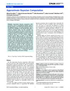
Importance Sampling estimates of P(M=1|y) Fig. 2.

Same caption as Fig. 1 when using 15 summary statistics.

ring the distinction between ABC and likelihood-based estimates but also reassuring the ability of ABC to provide the right choice of model with a higher information content of the data. We note that, for this experiment, all ABC-based decisions conclude in favor of the correct model. As shown in Fig. S6, this second experiment requires an increase in the number of importance sampling simulations because of a higher variability in the likelihood. Discussion Since its introduction by refs. 1 and 5, ABC has been extensively used in areas involving complex likelihoods, both for point estimation and testing of hypotheses. In realistic settings, with the exception of models such as Gibbs random fields, which are resilient with respect to their sufficient statistics, the conclusions drawn on model comparison cannot be trusted per se but require further simulation analyses as to the pertinence of the (ABC) Bayes factor based on the summary statistics. This paper has 1.0

0.0

0.2

0.4

0.6

0.8

1.0

Importance Sampling estimates of P(M=1|y)

0.6 0.4 0.2 0.0

ABC estimates of P(M=1|y)

0.8

0.8 0.6 0.4 0.2 0.0

ABC estimates of P(M=1|y)

0.2 0.0 0.0

1.0

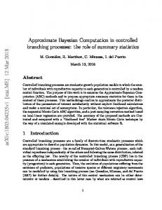
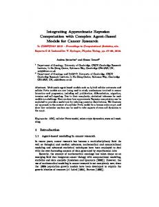
The second experiment also opposes two scenarios including three populations, two of them having diverged 100 generations ago and the third one resulting from a recent admixture between the first two populations (scenario 1) or simply diverging from population 1 (scenario 2) at the same time of 5 generations in the past. In scenario 1, the admixture rate is 0.7 from population 1. Pseudo observed datasets (100) of the same size as in experiment 1 (15 diploid individuals per population, 5 independent microsatellite loci) have been generated for an effective population size of 1,000 and mutation rates of 0.0005. In contrast with experiment 1, analyses included the following six parameters (provided with corresponding priors): admixture rate (U½0.1;0.9
), three effective population sizes (U½200;2000
), the time of admixture/ second divergence (U½1;10
), and the time of the first divergence (U½50;500
). To account for a higher complexity in the scenarios, the IS algorithm was performed with 10,000 coalescent trees per particle. Apart from this change, both ABC and likelihood analyses have been performed in the same way as experiment 1. Fig. 1 shows a reasonable fit between the exact posterior probability of model 1 (evaluated by IS) and the ABC approximation in the first experiment on most of the 100 simulated datasets, even though the ABC approximation is biased toward 0.5. When using 0.5 as the decision boundary between model 1 and model 2, there is hardly any discrepancy between both approaches, demonstrating that model choice based on ABC can be trusted in this case. Fig. 2 considers the same setting when moving from 24 to 15 summary statistics (given in Table S1): The fit somehow degrades. In particular, the number of opposite conclusions in the model choice moves to 12%. In the more complex setting of the second experiment, the discrepancy worsens, as shown in Fig. 3. The number of opposite conclusions reaches 26% and the fit between both versions of the posterior probabilities is considerably degraded, with a correlation coefficient of 0.643. The validity of the importance sampling approximation can obviously be questioned in both experiments; however, Figs. S3 and S4 display a strong stability of the posterior probability IS approximation across 10 independent runs for 5 different datasets and give proper confidence in this approach. Increasing the number of loci to 50 and the sample size to 100 individuals per population (see SI Text) leads to posterior probabilities of the true scenario overwhelmingly close to one (Fig. S5), thus blur-

0.0

0.2

0.4

0.6

0.8

1.0

Importance Sampling estimates of P(M=1|y) Fig. 1. Comparison of IS and ABC estimates of the posterior probability of scenario 1 in the first population genetic experiment, using 24 summary statistics. 15116 ∣

www.pnas.org/cgi/doi/10.1073/pnas.1102900108

Fig. 3. Comparison of IS and ABC estimates of the posterior probability of scenario 1 in the second population genetic experiment.

Robert et al.

1. Tavaré S, Balding D, Griffith R, Donnelly P (1997) Inferring coalescence times from DNA sequence data. Genetics 145:505–518. 2. Beaumont M, Zhang W, Balding D (2002) Approximate Bayesian computation in population genetics. Genetics 162:2025–2035. 3. Cornuet JM, et al. (2008) Inferring population history with DIYABC: A user-friendly approach to Approximate Bayesian Computation. Bioinformatics 24:2713–2719. 4. Robert C, Casella G (2004) Monte Carlo Statistical Methods (Springer, New York), 2nd Ed. 5. Pritchard J, Seielstad M, Perez-Lezaun A, Feldman M (1999) Population growth of human Y chromosomes: A study of Y chromosome microsatellites. Mol Biol Evol 16:1791–1798. 6. Beaumont M (2010) Approximate Bayesian computation in evolution and ecology. Annu Rev Ecol Evol Syst 41:379–406. 7. Lopes J, Beaumont M (2010) ABC: A useful Bayesian tool for the analysis of population data. Infect Genet Evol 10:825–832. 8. Csillèry K, Blum M, Gaggiotti O, François O (2010) Approximate Bayesian computation (ABC) in practice. Trends Ecol Evol 25:410–418. 9. Ratmann O, Andrieu C, Wiujf C, Richardson S (2009) Model criticism based on likelihood-free inference, with an application to protein network evolution. Proc Natl Acad Sci USA 106:1–6. 10. Templeton A (2009) Statistical hypothesis testing in intraspecific phylogeography: Nested clade phylogeographical analysis vs approximate Bayesian computation. Mol Ecol 18:319–331. 11. Templeton A (2010) Coherent and incoherent inference in phylogeography and human evolution. Proc Natl Acad Sci USA 107:6376–6381. 12. Beaumont M, et al. (2010) In defense of model-based inference in phylogeography. Mol Ecol 19:436–446. 13. Csillèry K, Blum M, Gaggiotti O, François O (2010) Invalid arguments against ABC: A reply to A. R. Templeton. Trends Ecol Evol 25:490–491. 14. Berger J, Fienberg S, Raftery A, Robert C (2010) Incoherent phylogeographic inference. Proc Natl Acad Sci USA 107:E57. 15. Lehmann E, Casella G (1998) Theory of Point Estimation (revised edition) (Springer, New York). 16. Fearnhead P, Prangle D Semi-automatic approximate Bayesian computation. J Royal Statist Soc, in press. 17. Joyce P, Marjoram P (2008) Approximately sufficient statistics and Bayesian computation. Stat Appl Genet Mol Biol 7:article 26. 18. Nunes MA, Balding DJ (2010) On optimal selection of summary statistics for approximate Bayesian computation. Stat Appl Genet Mol Biol 9:article 34. 19. Jeffreys H (1939) Theory of Probability (Clarendon Press, Oxford, UK), 1st Ed. 20. Estoup A, Beaumont M, Sennedot F, Moritz C, Cornuet J (2004) Genetic analysis of complex demographic scenarios: Spatially expanding populations of the cane toad, Bufo Marinus. Evolution 58:2021–2036. 21. Miller N, et al. (2005) Multiple transatlantic introductions of the Western corn rootworm. Science 310:992. 22. Pascual M, et al. (2007) Introduction history of Drosophila subobscura in the New World: A microsatellite-based survey using ABC methods. Mol Ecol 16:3069–3083. 23. Sainudiin R, et al. (2011) Experiments with the site frequency spectrum. Bull Math Biol 73:829–872. 24. Fagundes N, et al. (2007) Statistical evaluation of alternative models of human evolution. Proc Natl Acad Sci USA 104:17614–17619.

25. Grelaud A, Marin JM, Robert C, Rodolphe F, Tally F (2009) Likelihood-free methods for model choice in Gibbs random fields. Bayesian Anal 3:427–442. 26. Toni T, Welch D, Strelkowa N, Ipsen A, Stumpf M (2009) Approximate Bayesian computation scheme for parameter inference and model selection in dynamical systems. J R Soc Interf 6:187–202. 27. Belle E, Benazzo A, Ghirotto S, Colonna V, Barbujani G (2008) Comparing models on the genealogical relationships among Neandertal, Cro-Magnoid and modern Europeans by serial coalescent simulations. Heredity 102:218–225. 28. Cornuet JM, Ravigné V, Estoup A (2010) Inference on population history and model checking using DNA sequence and microsatellite data with the software DIYABC (v10). BMC Bioinformatics 11:401. 29. Excoffier C, Leuenberger D, Wegmann L (2009) Bayesian computation and model selection in population genetics. arXiv:0901.2231. 30. Ghirotto S, et al. (2010) Inferring genealogical processes from patterns of bronze-age and modern DNA variation in Sardinia. Mol Biol Evol 27:875–886. 31. Guillemaud T, Beaumont M, Ciosi M, Cornuet JM, Estoup A (2009) Inferring introduction routes of invasive species using approximate Bayesian computation on microsatellite data. Heredity 104:88–99. 32. Leuenberger C, Wegmann D (2010) Bayesian computation and model selection without likelihoods. Genetics 184:243–252. 33. Patin E, et al. (2009) Inferring the demographic history of African farmers and Pygmy hunter-gatherers using a multilocus resequencing data set. PLoS Genetics 5:e1000448. 34. Ramakrishnan U, Hadly E (2009) Using phylochronology to reveal cryptic population histories: Review and synthesis of 29 ancient DNA studies. Mol Ecol 18:1310–1330. 35. Verdu P, et al. (2009) Origins and genetic diversity of Pygmy hunter-gatherers from western central Africa. Curr Biol 19:312–318. 36. Wegmann D, Excoffier L (2010) Bayesian inference of the demographic history of chimpanzees. Mol Biol Evol 27:1425–1435. 37. Wegmann D, Leuenberger C, Neuenschwander S, Excoffier L (2010) ABCtoolbox: A versatile toolkit for approximate Bayesian computations. BMC Bioinformatics 11:116–123. 38. Lopes JS, Balding D, Beaumont MA (2009) PopABC: A program to infer historical demographic parameters. Bioinformatics 25:2747–2749. 39. Toni T, Stumpf M (2010) Simulation-based model selection for dynamical systems in systems and population biology. Bioinformatics 26:104–110. 40. Didelot X, Everitt R, Johansen A, Lawson D (2011) Likelihood-free estimation of model evidence. Bayesian Anal 6:1–28. 41. Bernardo J, Smith A (1994) Bayesian Theory (John Wiley, New York). 42. Wilkinson RD (2008) Approximate Bayesian computation (ABC) gives exact results under the assumption of model error. arXiv:0811.3355. 43. Sousa V, Fritz M, Beaumont M, Chikhi L (2009) Approximate Bayesian computation without summary statistics: the case of admixture. Genetics 181:1507–1519. 44. Dean T, Singh S, Jasra A, Peters G (2011) Parameter estimation for hidden Markov models with intractable likelihoods. arXiv:1103.5399. 45. Marin J, Pudlo P, Robert C, Ryder R (2011) Approximate Bayesian computational methods. Stat Comput, in press. 46. Estoup A, Clegg S (2003) Bayesian inferences on the recent island colonization history by the bird Zosterops lateralis lateralis. Mol Ecol 12:657–674. 47. Lombaert E, et al. (2010) Bridgehead effect in the worldwide invasion of the biocontrol Harlequin Ladybird. PloS ONE 5:e9743. 48. Stephens D, Donnelly P (2000) Inference in population genetics (with discussion). J R Stat Soc Series B Stat Methodol 62:602–655.

Robert et al.

PNAS ∣ September 13, 2011 ∣

vol. 108 ∣

no. 37 ∣

15117

BIOPHYSICS AND COMPUTATIONAL BIOLOGY

ACKNOWLEDGMENTS. The authors are grateful to the reviewers and to Michael Stumpf for their comments. Computations were performed on the INRA CBGP and MIGALE clusters. C.P.R., J.-M.C., and J-M.M. have been partly supported by Agence Nationale de la Recherche via the 2009–2013 project EMILE (Études de Méthodes Inférentielles et Logiciels pour l’Évolution). N.S.P. gratefully acknowledges National Science Foundation Grant DMS 1107070.

STATISTICS

tion rates resulting from using the ABC posterior probabilities in selecting a model as the most likely. For instance, in the setting of both our population genetic experiments, DIY-ABC gives false allocation rates equal to 20% (under scenarios 1 and 2) and 14.5% and 12.5% (under scenarios 1 and 2), respectively. This evaluation obviously shifts away from the performances of ABC as an approximation to the posterior probability toward the performances of the whole Bayesian apparatus for selecting a model, but this nonetheless represents a useful and manageable quality assessment for practitioners.

examined in details only the case when the summary statistics are sufficient for both models, while practical situations imply the use of insufficient statistics. The rapidly increasing number of applications estimating posterior probabilities by ABC indicates a clear need for further evaluations of the worth of those estimations, especially because our population genetic experiments showed that those ABC approximations were selecting the proper model. Further research is needed for producing trustworthy approximations to the posterior probabilities of models. At this stage, unless the whole data are involved in the ABC approximation as in ref. 43, our conclusion on ABC-based model choice is to exploit the approximations in an exploratory manner as measures of discrepancies rather than genuine posterior probabilities. This direction relates with the analyses found in ref. 9. Furthermore, a version of this exploratory analysis is already provided in the DIY-ABC software of ref. 3. An option in this software allows for the computation of a Monte Carlo evaluation of false alloca-