Learning a Wavelet-like Auto-Encoder to Accelerate Deep Neural ...

Learning a Wavelet-like Auto-Encoder to Accelerate Deep Neural Networks Tianshui Chen1 , Liang Lin1,5∗ , Wangmeng Zuo2 , Xiaonan Luo3 , Lei Zhang4 1

School of Data and Computer Science, Sun Yat-sen University, Guangzhou, China School of Computer Science and Technology, Harbin Institute of Technology, Harbin, China 3 School of Computer Science and Information Security, Guilin University of Electronic Technology, Guilin, China 4 Department of Computing, The Hong Kong Polytechnic University, HongKong 5 SenseTime Group Limited

arXiv:1712.07493v1 [cs.CV] 20 Dec 2017

2

Methods

top-5 err.

CPU (ms)

GPU (ms)

#FLOPs

VGG16 (224) VGG16 (112) Ours

11.65 15.73 11.87

1289.28 340.73 (3.78×) 411.63 (3.13×)

6.15 1.57 (3.92×) 2.37 (2.59×)

15.36B 3.89B 4.11B

Abstract Accelerating deep neural networks (DNNs) has been attracting increasing attention as it can benefit a wide range of applications, e.g., enabling mobile systems with limited computing resources to own powerful visual recognition ability. A practical strategy to this goal usually relies on a two-stage process: operating on the trained DNNs (e.g., approximating the convolutional filters with tensor decomposition) and finetuning the amended network, leading to difficulty in balancing the trade-off between acceleration and maintaining recognition performance. In this work, aiming at a general and comprehensive way for neural network acceleration, we develop a Wavelet-like Auto-Encoder (WAE) that decomposes the original input image into two low-resolution channels (sub-images) and incorporate the WAE into the classification neural networks for joint training. The two decomposed channels, in particular, are encoded to carry the low-frequency information (e.g., image profiles) and high-frequency (e.g., image details or noises), respectively, and enable reconstructing the original input image through the decoding process. Then, we feed the low-frequency channel into a standard classification network such as VGG or ResNet and employ a very lightweight network to fuse with the high-frequency channel to obtain the classification result. Compared to existing DNN acceleration solutions, our framework has the following advantages: i) it is tolerant to any existing convolutional neural networks for classification without amending their structures; ii) the WAE provides an interpretable way to preserve the main components of the input image for classification.

Introduction Deep convolutional neural networks (CNNs) (LeCun et al. 1990; Krizhevsky, Sutskever, and Hinton 2012) have been continuously improving the performance of various vision tasks (Simonyan and Zisserman 2014; He et al. 2016; Long, Shelhamer, and Darrell 2015; Lin et al. 2017a; Chen et al. ∗ Corresponding author is Liang Lin (Email: [email protected]). This work was supported by State Key Development Program under Grant 2016YFB1001004, the National Natural Science Foundation of China under Grant 61622214 and Grant 61320106008, Special Program of the NSFC-Guangdong Joint Fund for Applied Research on Super Computation (the second phase), and Guangdong Natural Science Foundation Project for Research Teams under Grant 2017A030312006. c 2018, Association for the Advancement of Artificial Copyright Intelligence (www.aaai.org). All rights reserved.

Table 1: The top-5 error rate (%), execution time on CPU and GPU, FLOPs of VGG16-Net with 224 × 224 and 112 × 112 as input, and our model on the ImageNet dataset. B denotes billion. The error rate is measured on single-view without data augmentation. In the brackets are the acceleration rates compared with the standard VGG16-Net. The execution time is computed with a C++ implementation on Intel i7 CPU (3.50GHz) and Nvidia GeForce GTX TITAN-X GPU. 2016; Chen, Guo, and Lai 2016), but at the expense of significantly increased computational complexity. For example, the VGG16-Net (Simonyan and Zisserman 2014), which has demonstrated remarkable performance on a wide range of recognition tasks (Long, Shelhamer, and Darrell 2015; Ren et al. 2015; Wang et al. 2017), requires about 15.36 billion FLOPs1 to classify an 224×224 image. These costs can be prohibitive for the deployment on ordinary personal computers and mobile devices with limited computing resources. Thus, it is highly essential to accelerate the deep CNNs. There have been a series of efforts dedicated to speed up the deep CNNs, most of which (Lebedev et al. 2014; Tai et al. 2015) employ tensor decomposition to accelerate convolution operations. Typically, these methods conduct two-step optimization separately: approximating the convolution filters of a pre-trained CNN with low-rank decomposition, and then fine-tuning the amended network. This would lead to difficulty in balancing the trade-off between acceleration rate and recognition performance, because two components are not jointly learned to maximize their strengths through cooperation. Another category of algorithms that aim at network acceleration is weight and activation quantization (Rastegari et al. 2016; Cai et al. 2017; Chen et al. 2015), but they usually suffer from an evident drop in performance despite yielding significant speed-up. For example, XNOR-Net (Rastegari et al. 2016) achieves 58× speed-up but undergoes 16.0% top-5 accuracy drop by ResNet-18 on the ImageNet dataset (Russakovsky et al. 2015). Therefore, we present our method according to the 1

FLOPs is the number of FLoating-point OPerations

following two principles: 1) no explicit network modification such as filter approximation or weight quantitation is needed, which helps to easily generalize to networks with different architectures; 2) the network should enjoy desirable speed-up with tolerable deterioration in performance. Since the FLOPs is directly related to the resolution of input images, a seemingly plausible way for acceleration is down-sampling the input images during both training and testing procedures. Although achieving a significant speedup, it inevitably suffers from a drastic drop in performance due to the loss of information (see Table 1). To address this dilemma, we develop a Wavelet-like Auto-Encoder (WAE) that decomposes the original input image into two lowresolution channels and feeds them into the deep CNNs for acceleration. Two decomposed channels are constrained to have following properties: 1) they are encoded to carry lowfrequency and high-frequency information, respectively, and are enabled to reconstruct the original image through a decoding process. Thus, most of the content from the original image can be preserved to ensure recognition performance; 2) the high-frequency channel carries minimum information, and thus we can use a lightweight network on it to avoid incurring massive computational burden. In this way, the WAE consists of an encoding layer that decomposes the input image into two channels, and a decoding layer to synthesize the original image based on these two channels. A transform loss, which includes a reconstruction error between the input image and the synthesized image, and an energy minimization loss on the high-frequency channel, is defined to optimize the WAE jointly. Finally, we feed the low-frequency channel to a standard network (e.g., VGG16-Net (Simonyan and Zisserman 2014), ResNet (He et al. 2016)), and employ a lightweight network to fuse with the high-frequency channel for the classification result. In the experiments, we first apply our method to the widely used VGG16-Net and conduct extensive evaluations on two large-scale datasets, i.e., the ImageNet dataset for image classification and the CACD dataset for face identification. Our method achieves an acceleration rate of 3.13 with merely 0.22% top-5 accuracy drop on ImageNet (see Tabel 1). On CACD, it even beats the VGG16-Net in performance while achieving the same acceleration rate. Similar experiments with ResNet-50 reveal that even for more compact and deeper network, our method can still achieve 1.88× speed-up with only 0.8% top-5 accuracy drop on ImageNet. Note that our method also achieves a better tradeoff between accuracy and speed compared with state-ofthe-art methods on both VGG16-Net and ResNet. Besides, our method exhibits amazing anti-noise ability compared with the standard network that takes original images as input. Codes are available at https://github.com/ tianshuichen/Wavelet-like-Auto-Encoder.

al. (Rigamonti et al. 2013) approximate the filters of a pretrained CNNs with a linear combination of low-rank filters. Jaderberg et al. (Jaderberg, Vedaldi, and Zisserman 2014) devise a basis of low-rank filters that are separable in the spatial domain and further develop two different schemes to learn these filters, i.e.,“Filter reconstruction” that minimizes the error of filter weights and “Data reconstruction” that minimizes the error of the output responses. Lebedev et al. (Lebedev et al. 2014) adopt a two-stage method that first approximates the convolution kernels using the low-rank CPdecomposition, and then fine-tunes the amended CNN. Quantization and Pruning. Weight and activation quantization are widely used for network compression and acceleration. As a representative work, XNOR-Net (Rastegari et al. 2016) binarizes the input to convolutional layers and filter weights, and approximates convolutions using primarily binary operations, resulting in significant speed-up but an evident drop in performance. Cai et al. (Cai et al. 2017) further introduce Half-Wave Gaussian Quantization to improve the performance of this method. On the other hand, pruning the unimportant connections or filters can also compress and accelerate deep networks. Han et al. (Han, Mao, and Dally 2015) remove the connections with weights below a threshold, reducing the parameters by up to 13×. This method is further combined with weight quantization to achieve an even higher compression rate. Similarly, Li et al. (Li et al. 2016) measure the importance of a filter by calculating its absolute weight sum and remove the filters with small sum values. Molchanov et al. (Molchanov et al. 2016) employ the Taylor expansion to approximate the change in the cost function induced by pruning filters. Luo et al. (Luo, Wu, and Lin 2017) further formulate filter pruning as an optimization problem. Network structures. Some works explore more optimal network structures for efficient training and inference. Lin et al. (Lin, Chen, and Yan 2013) develop a low-dimensional embedding method to reduce the number and size of the filters. Simonyan et al. (Simonyan and Zisserman 2014) show that stacked filters with small spatial dimensions (e.g., 3×3) could operate in the same receptive field of larger filters (e.g., 5 × 5) with less computational complexity. Iandola et al. (Iandola et al. 2016) further replace some 3 × 3 filters with 1 × 1 filters, and decrease the number of input channels to 3 × 3 filters to simultaneously speed up and compress the deep networks. Different from the aforementioned methods, we learn a WAE that decomposes the input image into two lowresolution channels and utilizes these decomposed channels as inputs to the CNN to reduce the computational complexity without compromising accuracy. Compared with existing methods, our method does not amend the network structures, and thus it can easily generalize to any existing convolutional neural networks.

Related Work Tensor decomposition. Most of the previous works for CNN acceleration focus on approximating the convolution filters by low-rank decomposition (Rigamonti et al. 2013; Jaderberg, Vedaldi, and Zisserman 2014; Lebedev et al. 2014; Tai et al. 2015). As a pioneering work, Rigamonti et

Proposed Method The overall framework of our proposed method is illustrated in Figure 1. The WAE decomposes the input image into two low-resolution channels that carry low-frequency information (e.g., basic profile) and high-frequency (e.g., auxiliary

Wavelet-like Auto-Encoder Reconstruction: ℓ$ = 𝐼 − 𝐼 "

' '

Energy: ℓ( = 𝐼)

𝐼)

Encoding layer

' '

Decoding layer Synthesized image 𝐼 "

Input image 𝐼

𝐼* …

Fusion

.. . Output

Standard classification net

Figure 1: The overall framework of our proposed method. The key component of the framework is the WAE that decomposes an input image into two low-resolution channels, i.e., IL and IH . These two channels encode the high- and low-frequency information respectively and are enabled to construct the original image via a decoding process. The low-frequency channel is then fed into the a standard network (e.g., VGG16-Net or ResNet) to extract its features. Then a lightweight network fuses these features and the high-frequency channel to predict the label scores. Note that the input to the classification network is low-resolution; thus it enjoys higher efficiency. Input image

details), i.e., IL and IH , and these two channels are enabled to construct the original image through the decoding process. Finally, the low-frequency channel is fed into a standard network (e.g., VGG16-Net or ResNet) to produce its features, and a network is further employed to fuse these features with the high-frequency channel to predict the classification result.

Wavelet-like Auto-Encoder The WAE consists of an encoding layer that decomposes the input image into two low-resolution channels and a decoding layer that synthesizes the original input image based on these two decomposed channels. In the following context, we introduce the image decomposition and synthesis processes in detail. Image decomposition. Given an input image I of size W × H, it is first decomposed into two half-resolution channels, i.e., IL and IH , which is formulated as: [IL , IH ] = FE (I, WE ),

(1)

where FE denotes the encoding process, and WE are its parameters. In this paper, the encoding layer contains three stacked convolutional (conv) layers with strides of 1, followed by two branched conv layers with strides of 2 to produce IL and IH , respectively. It is intolerable if this process incurs massive computational overhead, as we focus on acceleration. To ensure efficient computing, we utilize the small kernels with sizes of 3×3 and set the channel numbers of all intermediate layers as 16. The detailed architecture of the encoding layer are illustrated in Figure 2 (the blue part). Image synthesis. The decoding layer is employed to synthesize the input image based on IL and IH . It processes IL and IH to get the up-sampled images I 0 L and I 0 H , separately, and then simply adds them to obtain the synthesized

3×3 conv, 16 3×3 conv, 16 3×3 conv, 16 3×3 conv, 3, /2

3×3 conv, 3, /2

𝐼&

𝐼'

4×4 deconv, 16, ×2

4×4 deconv, 16, ×2

3×3 conv, 16

3×3 conv, 16

3×3 conv, 16

3×3 conv, 16

3×3 conv, 3

3×3 conv, 3

Element-wise sum Synthesized image

Figure 2: Detailed architecture of the wavelet-like autoencoder. It consists of an encoding (the blue part) and a decoding (the green part) layers. “/2” denotes a conv layer with a stride of 2 to downsample the feature maps, and conversely “×2” denotes a deconv layer with a stride of 2 to upsample the feature maps. image I 0 . The process is formulated as: I 0 = FDL (IL , WDL ) + FDH (IH , WDH ),

(2)

where FDL and FDH are the transforms on IL and IH , and WDL and WDH are their parameters. The decoding layer has two branches that share the same architecture, with each branch implementing one transform. Each branch contains a

deconvolutional (deconv) layer with a stride of 2 and three stacked conv layers with strides of 1, in which the deconv layer first up-samples the input images (i.e., IL and IH ) by two times, and the conv layers further refine the up-sampled feature maps to generate the outputs (i.e., I 0 L and I 0 H ). We set the kernel size of the deconv layer as 4 × 4, and those of the conv layers as 3×3. The channel numbers of all the intermediate layers are also set as 16. We present the detailed architecture of the decoding layer in Figure 2 (the green part).

Encoding and decoding constraints We adopt the two decomposed channels IL and IH to replace the original image as input to the classification network. To ensure the classification performance and simultaneously consider the computational overhead, IL and IH are expected to possess two properties as follows: • Minimum information loss. IL and IH should retain all the content of the original image as the classification network does not see the original image directly. If some discriminative content is lost unexpectedly, it may lead to classification error. • Minimum IH energy. IH should contain minimum information, so we can apply a lightweight network to it to avoid incurring heavy computational overhead. To comprehensively consider these two properties, we define a transform loss that consists of two simple yet effective constraints on the decomposed and reconstructed results. Reconstruction constraint. An intuitive assumption is that if IL and IH preserve all the content of the input image, they are enabled to construct the input image. In this paper, we reconstruct image I 0 from IL and IH through the decoding process, and minimize the reconstruction error between input image I and reconstructed image I 0 . So the reconstruction constraint can be formulated as:

the standard network except that the channel numbers of all the conv layers are divided by 4. fL is fed into a simple classifier to predict a score vector sL , and it is further concatenated with fH to compute a score vector sc by a similar classifier. The two vectors are then averaged to obtain the final score vector s. We employ the cross entropy loss as our objective function to train the classification network. Suppose there are N training samples, and each sample Ii is annotated with a label yi . Given the predicted probability vector pi exp(sc ) pci = PC−1 i 0 c = 0, 1, . . . , C − 1, c c0 =0 exp(si )

(6)

where C is the number of class labels. The classification loss function is expressed as: L1 = −

N C−1 1 XX 1(yi = c) log pc , N i=1 c=0

(7)

where 1(·) is the indicator function whose value is 1 when the expression is true, and 0 otherwise. We use the same loss function for sc and sL and simply sum up them to get the final classification loss Lc . Discussion on computational complexity. As suggested in (He and Sun 2015), the convolutional layers often take 90-95% computational cost. Here, we analyze the computational complexity of the convolutional layers and present an up bound of the acceleration rate of our method compared with the standard network. For a given CNN, the total complexity of all the convolutional layers can be expressed as: d X nl−1 · s2l · nl · m2l ), O(

(8)

l=1

Lt = `r + λ`e , (5) where λ is a weighted parameter, and it is set as 1 in our experiments.

where d is the number of the conv layers, and l is the index of the conv layer; nl is the channel number of the l-th layer; sl is the spatial size of the kernels and ml is the spatial size of the output feature maps. For the standard network, as it takes a half-resolution image as input, ml of each layer is also halved. So the computational complexity is about 14 of the standard network that takes original images as input. For the sub-module in fusion network that processes IH , the channel number of all the corresponding layers are further quar1 tered, so the computational complexity is merely about 64 of the original standard network. So the up bound of the acceleration rate of our classification network compared with 1 the standard network can be estimated by 1/4+1/64 = 3.76. However, as the decomposition process and additional fullyconnected layers could incur additional overhead, the actual acceleration rate may be lower than 3.76.

Image classification

Learning

The image classification network consists of a standard network to extract the features fL for IL , and a fusion network to fuse with IH to predict the final label scores. Here, the standard network refers to the VGG16-Net or the ResNet, and we use the features maps from the last conv layer. The fusion network contains a sub-module to extract features fH for IH . The sub-module shares the same architecture with

Our model is comprised of the WAE and the classification network, and it is indeed possible to jointly train them using a combination of the transform and classification losses in an end-to-end manner. However, it is difficult to balance the two loss terms if directly training from scratch, inevitably leading to inferior performance. To address this issue, the training process is empirically divided into three stages:

`r = ||I − I 0 ||22 . (3) Energy constraint. The second constraint minimizes the energy of IH and pushes most information to IL thus that IH preserves minimum content. It can be formulated as: `e = ||IH ||22 . (4) We combine the two constraints on the decomposed and reconstructed results to define a transform loss. It is formulated as the weighted sum of these two constraints:

Stage 1: WAE training. We first remove the classification network and train the WAE using the transform loss Lt . Given an image, we first resize it to 256 × 256 and randomly extract patches (and their horizontal reflections) with a size of 224 × 224, and train the network based on these extracted patches. The parameters are initialized with the Xavier algorithm (Glorot and Bengio 2010) and the WAE is trained using SGD algorithm with a mini-batch of 4, momentum of 0.9 and weight decay of 0.0005. We set the initial learning rate as 0.000001, and divide it by 10 after 10 epochs. Stage 2: Classification network training. We combine the classification network with the WAE, and train the classification network with the classification loss Lc . The parameters of the WAE are initialized with the parameters learned in Stage 1 and are kept fixed, and the parameters of classification network are also initialized with the Xavier algorithm. The training images are resized to 256 × 256, and the same strategies (i.e., random cropping and horizontal flipping) are adopted for data augmentation. The network is also trained using SGD algorithm with the same momentum and weight decay as Stage 1. The mini-batch is set as 256, and the learning rate is initialized as 0.01 (0.1 if using ResNet-50 as the baseline), which is divided by 10 when the error plateaus. Stage 3: Joint fine tuning. To better adapt the decomposed channels for classification, we also fine tune WAE and classification network jointly by combining the transform and classification losses, formulated as: L = Lc + γLt ,

(9)

where γ is set to be 0.001 to balance the two losses. The network is fine tuned using SGD with the mini-batch size, momentum, and weight decay the same as Stage 2. We utilize a small learning rate of 0.0001 and train the network until the error plateaus.

Experiments Baseline methods In the experiments, we utilize two popular standard networks, i.e., VGG16-Net and ResNet-50, as the baseline networks, and mainly compare with these baselines on image recognition performance and execution efficiency. To further validate the effectiveness of the proposed WAE, we implement two baseline methods that also utilize the decomposed channels as input to the deep CNNs for classification. Wavelet+CNN. Discrete wavelet transforms (DWTs) decompose an input image to four half-resolution channels, i.e., cA, cH, cV, cD, where cA is an approximation to the input image (similar to IL ), while cH, cV, cD preserve image details (similar to IH ). Also, the original image can be reconstructed based on cA, cH, cV, cD using an inverse transform. Then, cA is fed into the standard network, and cH, cV, cD is concatenated and fed into the final for classification. Here, we use the widely used 9/7 implementation (Zhang et al. 2011) for the DWT. Decomposition+CNN. This method also uses an encoding layer the same to that in our proposed WAE to decompose the input image into two half-resolution ones, followed by the classification network for predicting the class labels. But

it has no constraints on the decomposed channels, and it is trained merely with the classification loss. The classification networks in the two baseline methods share the same structure with that of ours for fair comparisons. Both two methods are also trained with SGD with an initial learning rate of 0.01, mini-batch of 256, momentum of 0.9 and weight decay of 0.0005. We select the models with lowest validation errors for comparison.

ImageNet classification with VGG16 We first evaluate our proposed method on VGG16-Net on the ImageNet dataset (Russakovsky et al. 2015). The dataset covers 1,000 classes and comprises a training set of about 1.28 million images and a validation set of 50,000 images. All the methods are trained on the training set, and evaluated on the validation set as the ground truth of the test set are not available. Following (Zhang et al. 2016), we report the top-5 error rate for performance comparison. Comparison with the original VGG16-Net We first compare the classification performance and execution time on CPU and GPU of our model and the original VGG16Net2 in Table 2. The execution time is evaluated with a C++ implementation on Intel i7 CPU (3.50GHz) and Nvidia GeForce GTX TITAN-X GPU. We can see our model achieves a speed-up rate of up to 3.13× with merely 0.22% increase in the top-5 error rate. For the CPU version, our model obtains an actual acceleration rate of 3.13×, close to the up bound of the acceleration rate (3.76×). The overhead may come from the computational cost of the encoding layer and additional fully-connected layers. For the GPU version, the actual acceleration rate is 2.59×. It is smaller since an accelerated model is harder for parallel computing. Comparison with state-of-the-art methods ThiNet (Luo, Wu, and Lin 2017) and Taylor3 (Molchanov et al. 2016) are two newest methods that also focus on accelerating deep CNNs, and they also conduct experiments on VGG16-Net. In this part, we compare our model with these methods and report the results in Table 2. Taylor presents two models, namely Taylor-1 and Taylor-2. Our model achieves better accuracy and speed-up rate than Taylor-1. The speed-up rate of Taylor-2 is a bit higher than ours, but it suffers an evident performance drop (3.63% increase in top-5 error rate). ThiNet also presents two models, i.e., ThiNet-GAP and ThiNet-Tiny. ThiNet-Tiny enjoys a significant speed-up at the cost of a drop in accuracy (6.47% increase in top-5 error rate), which is intolerant for real-world systems. ThiNet-GAP can achieve a better trade-off between speed and accuracy, but our model still surpasses it in both speed and accuracy. Comparison with the baseline methods To validate the effectiveness of the proposed WAE, we also compare our 2

For a fair comparison, the top-5 error rate of the original VGG16-Net is evaluated with center-cropped patches on resized images. The same strategy is also used in ResNet-50. 3 The execution time reported in Taylor paper are conducted on a hardware and software platform that is different from ours. Thus we merely present the relative speed-up rates for fair comparison.

Methods top-5 err. (%) CPU (ms) CPU speed-up rate GPU (ms) GPU speed-up rate VGG16-Net 11.65 1289.28 1× 6.15 1× Wavelet+CNN 14.42 392.24 3.29× 2.30 2.67× Decomposition+CNN 12.98 411.63 3.13× 2.37 2.59× Taylor-1 13.00 1.70× 2.20× Taylor-2 15.50 2.10× 3.40× ThiNet-Tiny 18.03 116.25 11.25× 1.32 4.66× ThiNet-GAP 12.08 442.807 2.91× 2.52 2.44× Ours 11.87 411.63 3.13× 2.37 2.59× Table 2: Comparison of the top-5 error rate, execution time and speed-up rate on CPU and GPU of VGG16-Net, the two baseline methods and the previous state of the art methods on the ImageNet dataset. The error rate is measured on single-view without data augmentation.

(a)

(b)

(c)

(d)

(e)

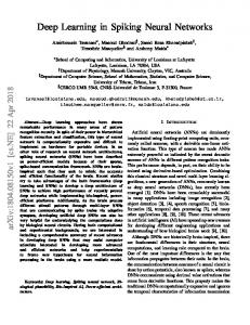
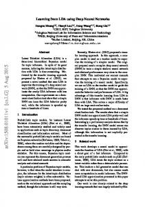
Figure 3: Visualization results of the input image (a), the sub-images (b) and (c) produced by our method and the subimages (d) and (e) produced by the “Decomposition+CNN”. model with two baseline methods that use different decomposition strategies in Table 2. It shows our model outperforms the two baseline methods by a sizable margin on the classification performance while sharing comparable efficiency. Note that “Wavelet+CNN” runs a bit faster than our method, as it uses the more efficient DWT for image decomposition. However, it results in inferior performance, and one possible reason is that directly separating the lowand high-frequency information of an image may hamper the classification result. Our model also decomposes the input image into two channels, but it pushes most information to the IL via minimizing the energy of IH and are jointly trained to better adapt for classification. We will conduct experiments to analyze the classification performance merely using IL and cA to give a deeper comparison later. To compare the difference between our model and the “Decomposition+CNN”, we visualize the decomposed channels generated by this method and ours in Figure 3. Without the constraints, the two decomposed channels share identical appearance, and fusing the classification results of them can be regarded as the model ensemble. Conversely, the channels generated by our model are somehow complementary, as IL retains the main content, while IH preserves the subtle details. These comparisons well prove the proposed WAE can achieve a better balance between speed and accuracy. Analysis on the decomposed channels Some examples of the decomposed channels and the reconstructed images are visualized in Figure 4. We can observe that IL indeed contains the main content of the input image, while IH preserves the details, e.g., edges and contours. It also shows

Input image

𝐼"

𝐼#

Reconstructed

Figure 4: Visualization results of the IL , IH and the reconstructed image. excellent reconstructed results. These visualization results finely accord with the assumption of our method. Input top-5 err.

cA 15.92

IR 15.73

IL 14.20

IL +IH 11.87

Table 3: Comparison of the top-5 error rate using IL +IH , IL , IR and cA for classification on the ImageNet dataset. To provide deeper analysis of the decomposed channels, we present the performance using the IL for classification. We first exclude the fusing with IH and re-train the classification network with the parameters of WAE fixed. The top-5 error rate is depicted in Table 3. It is not surprising that the performance drops, as IH preserves the image details and can provide auxiliary information for classification. We also conduct experiments that use cA generated by DWT, and IR generated by directly resizing the image to a given size, for classification. Specifically, we first resize cA and IR to 128 × 128, and randomly crop the patches of size 112 × 112 (and their horizontal reflections) for training. During testing, we crop the center patch with a size of 112 × 112 for fair comparisons. Although IL , IR and cA are all assumed to possess the main content of the original image, the classification result using IL is obviously superior to those using IR and cA. One possible reason is that the constraint on minimizing the energy of IH explicitly pushes most content to IL so that IL contains much more discriminative information than IR and cA. These comparisons can also give

a possible explanation that our approach outperforms the “Wavelet+CNN”. Contribution of joint fine tuning step We evaluated the contribution of joint fine tuning by comparing the performance with and without it, as reported in Table 4. The top-5 error rates with fine tuning decreases by 0.34%. This suggests fine tuning the network jointly can adapt the decomposed image for better classification. Methods top-5 err. (%)

w/o FT 12.21

ImageNet classification with ResNet-50 In this part, we further evaluate the performance of our proposed method on ResNet. Without loss of generalization, we select ResNet-50 from the ResNet family and simply use it to replace the VGG-Net as the baseline network. Then it is trained from scratch using a similar process as described in the Sec. of Learning. Because ResNet is a recently proposed network architecture, few works are proposed to accelerate this network. Thus, we simply compared with the standard ResNet-50, ThiNet in Table 5. ResNet is a more compact model, and accelerating this network is even more difficult. However, our method can still achieve 1.88× speed-up with merely 0.8% increase in top-5 error rate, surpassing ThiNet on both accuracy and efficiency. top-5 err. (%) 8.86 11.70 9.66

GPU SR 1× 1.30× 1.73×

Methods VGG16-Net Wavelet+CNN Decomposition+CNN Ours

acc. (%) 95.91 94.99 95.20 96.13

Table 6: Comparison of the accuracy of our model, VGG16Net and the baseline methods on the CACD dataset.

w/ FT 11.87

Table 4: Comparison of the top-5 error rate with and without joint fine tuning (FT) on the ImageNet dataset.

Methods ResNet-50 ThiNet-30 Ours

efficiency. It suggests our model can generalize to diverse datasets for accelerating the deep CNNs.

CPU SR 1× 1.88×

Table 5: Comparison of the top-5 error rate and speed-up rate (SR) of our model and ThiNet on ResNet-50 on the ImageNet dataset.

CACD face identification CACD is a large-scale and challenging dataset for face identification. It contains 163,446 images of 2,000 identities collected from the Internet that vary in age, pose and illumination. A subset of 56,138 images that cover 500 identities are manually annotated (Lin et al. 2017b). We randomly select 44,798 images as the training set and the rest as the test set. All the models are trained on the training set and evaluated on the test set. Table 6 presents the comparison results. Note that the execution times are the same as Table 2. In this dataset, our model outperforms the VGG16-Net (0.22% increase in accuracy) and meanwhile achieves a speed-up rate of 3.13×. Besides, our method also beats the baseline methods. These comparisons again demonstrate the superiority of our proposed WAE. Remarkably, the images on CACD are far different from those on ImageNet, and our method still achieves superior performance on both accuracy and

Noisy image classification Generally, the high-frequency part of an image contains more noise. Our model may implicitly remove some highfrequency part by minimize the energy of IH , so it may be inherently more robust to the noise. To validate this assumption, we add Gaussian noise of mean zero and different variances V to the test images, and present the accuracy of our method and the original VGG16-Net on these noisy images in Table 7. Note that both our model and the VGG16-Net is trained with the clean images. Our model performs consistently better than VGG16-Net over different noise levels. Remarkably, the superiority of our model is more evident when adding larger noise. For example, when adding noise with a variance of 0.05, our model outperforms the VGG16Net by 10.81% in accuracy. These comparisons suggest our method is more robust to noise compared to VGG16-Net. Methods V=0 V=0.01 V=0.02 V=0.05 V=0.1

VGG16-Net 95.91 90.22 80.00 45.10 14.31

Ours 96.13 91.16 83.85 55.91 23.88

Table 7: Comparison of accuracy (in %) on the image of our model and VGG16-Net with gaussian noise of zero mean and different variances on the CACD dataset.

Conclusion In this paper, we learn a Wavelet-like Auto-Encoder, which decomposes an input image into two low-resolution channels and utilizes the decomposed channels as inputs to the CNN to reduce the computational complexity without compromising the accuracy. Specifically, the WAE consists of an encoding layer to decompose the input image into two half-resolution channels and a decoding layer to synthesize the original image from the two decomposed channels. A transform loss, which combines a reconstruction error that constrains the two low-resolution channels to preserve all the information of the input image, and an energy minimization loss that constrain one channel contains minimum energy, are further proposed to optimize the network. In future work, we will conduct experiments to decompose the image into sub-images of lower resolution to explore a better trade-off between accuracy and speed.

References [Cai et al. 2017] Cai, Z.; He, X.; Sun, J.; and Vasconcelos, N. 2017. Deep learning with low precision by half-wave gaussian quantization. arXiv preprint arXiv:1702.00953. [Chen et al. 2015] Chen, W.; Wilson, J.; Tyree, S.; Weinberger, K.; and Chen, Y. 2015. Compressing neural networks with the hashing trick. In International Conference on Machine Learning, 2285–2294. [Chen et al. 2016] Chen, T.; Lin, L.; Liu, L.; Luo, X.; and Li, X. 2016. Disc: Deep image saliency computing via progressive representation learning. IEEE transactions on neural networks and learning systems 27(6):1135–1149. [Chen, Guo, and Lai 2016] Chen, S.-Z.; Guo, C.-C.; and Lai, J.-H. 2016. Deep ranking for person re-identification via joint representation learning. IEEE Transactions on Image Processing 25(5):2353–2367. [Glorot and Bengio 2010] Glorot, X., and Bengio, Y. 2010. Understanding the difficulty of training deep feedforward neural networks. In Aistats, volume 9, 249–256. [Han, Mao, and Dally 2015] Han, S.; Mao, H.; and Dally, W. J. 2015. Deep compression: Compressing deep neural networks with pruning, trained quantization and huffman coding. arXiv preprint arXiv:1510.00149. [He and Sun 2015] He, K., and Sun, J. 2015. Convolutional neural networks at constrained time cost. In Proceedings of the IEEE Conference on Computer Vision and Pattern Recognition, 5353–5360. [He et al. 2016] He, K.; Zhang, X.; Ren, S.; and Sun, J. 2016. Deep residual learning for image recognition. In Proceedings of the IEEE Conference on Computer Vision and Pattern Recognition, 770–778. [Iandola et al. 2016] Iandola, F. N.; Han, S.; Moskewicz, M. W.; Ashraf, K.; Dally, W. J.; and Keutzer, K. 2016. Squeezenet: Alexnet-level accuracy with 50x fewer parameters and¡ 0.5 mb model size. arXiv preprint arXiv:1602.07360. [Jaderberg, Vedaldi, and Zisserman 2014] Jaderberg, M.; Vedaldi, A.; and Zisserman, A. 2014. Speeding up convolutional neural networks with low rank expansions. arXiv preprint arXiv:1405.3866. [Krizhevsky, Sutskever, and Hinton 2012] Krizhevsky, A.; Sutskever, I.; and Hinton, G. E. 2012. Imagenet classification with deep convolutional neural networks. In Advances in neural information processing systems, 1097–1105. [Lebedev et al. 2014] Lebedev, V.; Ganin, Y.; Rakhuba, M.; Oseledets, I.; and Lempitsky, V. 2014. Speeding-up convolutional neural networks using fine-tuned cp-decomposition. arXiv preprint arXiv:1412.6553. [LeCun et al. 1990] LeCun, Y.; Boser, B. E.; Denker, J. S.; Henderson, D.; Howard, R. E.; Hubbard, W. E.; and Jackel, L. D. 1990. Handwritten digit recognition with a backpropagation network. In Advances in neural information processing systems, 396–404. [Li et al. 2016] Li, H.; Kadav, A.; Durdanovic, I.; Samet, H.; and Graf, H. P. 2016. Pruning filters for efficient convnets. arXiv preprint arXiv:1608.08710.

[Lin et al. 2017a] Lin, L.; Wang, G.; Zuo, W.; Feng, X.; and Zhang, L. 2017a. Cross-domain visual matching via generalized similarity measure and feature learning. IEEE transactions on pattern analysis and machine intelligence 39(6):1089–1102. [Lin et al. 2017b] Lin, L.; Wang, K.; Meng, D.; Zuo, W.; and Zhang, L. 2017b. Active self-paced learning for costeffective and progressive face identification. IEEE Transactions on Pattern Analysis and Machine Intelligence. [Lin, Chen, and Yan 2013] Lin, M.; Chen, Q.; and Yan, S. 2013. Network in network. arXiv preprint arXiv:1312.4400. [Long, Shelhamer, and Darrell 2015] Long, J.; Shelhamer, E.; and Darrell, T. 2015. Fully convolutional networks for semantic segmentation. In Proceedings of the IEEE Conference on Computer Vision and Pattern Recognition, 3431– 3440. [Luo, Wu, and Lin 2017] Luo, J.-H.; Wu, J.; and Lin, W. 2017. Thinet: A filter level pruning method for deep neural network compression. Proceedings of the IEEE international conference on computer vision. [Molchanov et al. 2016] Molchanov, P.; Tyree, S.; Karras, T.; Aila, T.; and Kautz, J. 2016. Pruning convolutional neural networks for resource efficient transfer learning. arXiv preprint arXiv:1611.06440. [Rastegari et al. 2016] Rastegari, M.; Ordonez, V.; Redmon, J.; and Farhadi, A. 2016. Xnor-net: Imagenet classification using binary convolutional neural networks. In European Conference on Computer Vision, 525–542. Springer. [Ren et al. 2015] Ren, S.; He, K.; Girshick, R.; and Sun, J. 2015. Faster r-cnn: Towards real-time object detection with region proposal networks. In Advances in neural information processing systems, 91–99. [Rigamonti et al. 2013] Rigamonti, R.; Sironi, A.; Lepetit, V.; and Fua, P. 2013. Learning separable filters. In Proceedings of the IEEE Conference on Computer Vision and Pattern Recognition, 2754–2761. [Russakovsky et al. 2015] Russakovsky, O.; Deng, J.; Su, H.; Krause, J.; Satheesh, S.; Ma, S.; Huang, Z.; Karpathy, A.; Khosla, A.; Bernstein, M.; et al. 2015. Imagenet large scale visual recognition challenge. International Journal of Computer Vision 115(3):211–252. [Simonyan and Zisserman 2014] Simonyan, K., and Zisserman, A. 2014. Very deep convolutional networks for largescale image recognition. arXiv preprint arXiv:1409.1556. [Tai et al. 2015] Tai, C.; Xiao, T.; Zhang, Y.; Wang, X.; et al. 2015. Convolutional neural networks with low-rank regularization. arXiv preprint arXiv:1511.06067. [Wang et al. 2017] Wang, Z.; Chen, T.; Li, G.; Xu, R.; and Lin, L. 2017. Multi-label image recognition by recurrently discovering attentional regions. In Proceedings of the IEEE Conference on Computer Vision and Pattern Recognition, 464–472. [Zhang et al. 2011] Zhang, L.; Zhang, L.; Mou, X.; and Zhang, D. 2011. Fsim: A feature similarity index for image quality assessment. IEEE transactions on Image Processing 20(8):2378–2386.

[Zhang et al. 2016] Zhang, X.; Zou, J.; He, K.; and Sun, J. 2016. Accelerating very deep convolutional networks for classification and detection. IEEE transactions on pattern analysis and machine intelligence 38(10):1943–1955.