LEAST SQUARE SUPPORT VECTOR MACHINE ALTERNATIVE TO ...

z

Available online at http://www.journalcra.com

INTERNATIONAL JOURNAL OF CURRENT RESEARCH International Journal of Current Research Vol. 4, Issue, 12, pp. 399-404, December, 2012

ISSN: 0975-833X

RESEARCH ARTICLE

LEAST SQUARE SUPPORT VECTOR MACHINE ALTERNATIVE TO ARTIFICIAL NEURAL NETWORK FOR PREDICTION OF SURFACE ROUGHNESS AND POROSITY OF PLASMA SPRAYED COPPER SUBSTRATES 1*Ajit

Behera, 2Sudeep Behera, 3Rajesh Kumar Tripathy, 4Subash Chandra Mishra

1,4Department

of Metallurgical and Materials Engineering Indian Institute of Technology, Kharagpur-721302, India 2Department of Electrical Engineering 3Department of Biomedical Engineering *Corresponding author: [email protected] ARTICLE INFO Article History: th

Received 10 September, 2012 Received in revised form 20th October, 2012 Accepted 23rd November, 2012 Published online 28th December, 2012

Key words: Plasma Spraying, Surface roughness, Porosity, Copper, LS-SVM, ANN.

ABSTRACT Plasma spraying technique has become a subject of intense research in many industrial structural/functional applications because its peculiarity surface properties. This investigation explains about plasma sprayed copper surface property. Here industrial waste and low grade ore (i.e. Flay-ash+ quartz+ illmenite), used as deposit material which is to be coated on copper substrates. In many applications, it is found that for structural modification, surface roughness & porosity parameters are very important. To decrease both surface roughness and coating porosity by optimizing other necessary properties, different soft computing methods like Artificial Neural Network (ANN) and Least Square support vector machine techniques used. The least square formulation of support vector machine (SVM) was recently proposed and rooted in the statistical learning theory. This technique potentially describes the approximation complexity of inter-relations between different parameters of atmospheric plasma spray process and helps in saving time & resources for experimental trials for which it is advantageous than all conventional methods. It is marked as a new development by learning from examples based on polynomial function, neural networks, radial basis function (RBF), splines or other function. From this above two methods (Multilayer Feed forward Neural Network& LS-SVM), we conclude that LS-SVM with RBF kernel gives better performance over ANN for prediction of surface roughness and coating porosity with minimum Mean Square Error. This methodology can provide clear understanding of various corelationships across multiple scales of length and time which could be essential for improvement of product performance and process. The results of this methodology give a good generalization capability to optimize the coating surface roughness& surface porosity. Copy Right, IJCR, 2012, Academic Journals. All rights reserved.

INTRODUCTION lasma sprayed technology have received much attention in recent years due to their outstanding surface properties when compared to those of their conventional processes. Plasma spray coating has the advantage of being able to process industrial waste and low-grade minerals to produce valueadded products (Satapathy et al., 2010), which are widely used in aerospace industry to biomedical industry (Hetmanczyk et al., 2007; Muggli et al., 1999; Behera, 2012a; Ohtsu, 2012) Plasma spray processes utilize the energy contained in a thermally ionized gas to melt prepared powder particle partially/fully and propel this molten/semi-molten powder on to a substrate surface such that they adhere and agglomerate to produce coatings. This technique implements a wide variety of materials (metal, ceramic, alloy and its composite) and processes (Atmospheric plasma spraying, vacuum plasma spraying etc.) for improving surface properties (Singla et al., 2011; Davis, 2004; Sampath et al., 2001). Conventional plasma-spraying refers to air or atmospheric plasma spraying (APS) process. Plasma generated by the help of an inert gas i.e.

argon or argon+ hydrogen mixture (Zhang et al., 2011). Approximately 6000°C to 15000°C temperature can generated in the power heating region, which is significantly above the melting point of any known material (Heimann, 2008). Homogenized powder mixture of fly-ash+ quartz+ illmenite having particle size from 40 µm to 100 µm injected into plasma flame and then accelerated with a very high velocity to impact on substrate surface in the form of molten/semi-molten state (Fauchais, 2004; Behera, 2012b). The coating efficiency directly or indirectly depends on many other parameters during spraying, in which each one is inter-related with each other. Porosity depends on several coating properties such as thermal conductivity, coefficient of thermal expansion, elastic modulus and dielectric behavior (Deshpande et al., 2004). Also surface roughness depends on particle state (molten/semi-molten), powder feeding rate etc. Various methods are employed for quantitative measurement of surface roughness & porosity and form a necessary part of micro structural characterization of thermal spray coatings. A variety of prediction models have been proposed in the manuscript that include time series models, regression models, adaptive neuro-fuzzy inference

400

International Journal of Current Research, Vol. 4, Issue, 12, pp. 399-404, December, 2012

systems (ANFIS), artificial neural network (ANN) models and SVM models. Among these model ANN increasingly used in different optimization process. This is mainly because the effectiveness and smoothness of ANN modeling systems, which improves a great deal in the engineering area. For classification and non-linear function estimation, the SVM is introduced by Vapnik (Vapnik, 1995; Vapnik, 1999). SVM have remarkable generalization performance and many more advantages over other methods, so SVM has attracted attention and gained extensive application. Suykens and Vandenwalle have proposed the use of the LS-SVM for simplification of traditional of SVM (Suykens et al., 2002). Not only LS-SVM has been used for classification in various areas of pattern recognition (Hanbay, 2009) but also it has handled regression problems successfully (Zuriani et al., 2011). LS-SVM has additional advantage as compared to SVM. In LS-SVM, a set of only linear equation (Linear programming) is solved which is much easier and computationally more simple. In this paper, by MFNN and LS-SVM models we are Predicting Surface Roughness and Porosity of Plasma Sprayed Copper. After comparing the result obtained by both these models, LS-SVM gives better performance to minimize the MSE that of MFNN. Experimental Procedure Flay-ash premixed with quartz and illuminate mixture taken (weight percentage ratio of 60:20:20) and homogenized by Planetary ball mill for 3 hour. This homogenized mixture used as coating material which is to be coated on Mild Steel substrate of dimension 3 mm thickness and 1 inch diameter. Four different sizes i.e. 40 µm, 60 µm, 80 µm and 100 µm are separated out by the application of sieve. Alumina grit blasting was made at a pressure of 3 kg/cm2 to create surface roughness of about 5Ra, for better bonding. By acetone substrates surface were cleaned which is followed by plasma spraying. The coating process made at the Laser & Plasma Technology Division, BARC, Mumbai. Here 40 kW DC non-transferred arc mode atmospheric plasma spray system used. Input power level varies from 11kW to 21 kW in spray gun. Coating powder material injects externally from the torch nozzle and directed towards the plasma flow. Ar/ H2/N2 gas may be used as carrier gas. The major subsystems of the set up include the plasma spraying torch, power supply, powder feeder, and carrier gas supply, torch to substrate surface distance, control console, cooling water and spray booth. A four stage closed loop centrifugal pump water cooling used for retrieving the heat generated during the process, regulated at a pressure of 10kg/cm2 supply. The specifications of spraying process parameters are given in table 1. Flow rate of plasma gas (Ar) and Secondary gas (N2) are kept constant. With increasing power level; powder feed rate, powder size and stand of distance of torch are varied. Measurement of coating surface roughness done by ‘Taylor/Hobson Surtronic 3+’ instrument and experimental value of porosity was measured by image analyzer technique. In image analyzer technique the porosity of coatings was measured by putting polished cross sections of the sample under a microscope (Neomate) equipped with a CCD camera (JVC, TK 870E). This system is used to obtain a digitized image of the object. The digitized image is transmitted to VOIS image analysis software. The total area captured by the

objective of the microscope or a fraction can be accurately measured by the software. Hence the total area and the area covered by the pores are separately measured. To find out some of the better surface property, there is a software programs used by implementation of MATLAB version 10.1. Back Propagation Algorithm (BPA) is used to train the network. The sigmoid function represented by equation (3.1) is used as the activation function for all the neurons except for those in the input layer. S(x) = 1 / (1+e-x)

(3.1)

Choice of Hidden Neurons The choice of optimal number of hidden neurons, Nh is the most interesting and challenging aspect in designing the MFNN. Simon Haykin (Simon, 1999) has specified that Nh should lie between 2 and ∞ (Hecht-Nielsen, 1990). HechtNielsen uses ANN interpretation of Kolmogorov’s theorem to arrive at the upper bound on the Nh for a single hidden layer network as 2(Ni+1), where Ni is the number of input neurons. However, this value should be decided very judiciously depending on the requirement of a problem. A large value of Nh may reduce the training error associated with the MFNN, but at the cost of increasing the computational complexity and time. For example, if one gets a tolerably low value of training error with certain value of Nh, there is no point in further increasing the value of Nh to enhance the performance of the MFNN. The input and the output data are normalized before being processed in the network as follows: In this scheme of normalization, the maximum values of the input and output vector components:

ni ,max  max  ni  p   p=1 …Np ,i= 1….Ni

(3.2)

Where Np is the number of patterns in the training set and Ni is the number of neurons in the input layer. Again, Ok ,max  max  ok  p   p=1,....Np, k=1,...Nk

(3.3)

Where, Nk is the number of neurons in the output layer. Normalized by these maximum values, the input and output variables are given as follows.

ni  p  , p = 1….N , i = 1,…N (3.4) p i ni,max and ok  p  , p = 1,...Np, i = 1,…Nk (3.5) ok ,nor  p   ok ,max After normalization, the input and output variable lay [13] in the range of 0 to 1. ni,nor  p  

Choice of ANN Parameters The learning rate, η and the momentum factor, α have a very significant effect on the learning speed of the BPA. The BPA provides an approximation to the trajectory in the weight space computed by the method of steepest descent method (Ghosh et al., 1999). If the value of η is considered very small, this results in slow rate of learning, while if the value of η is too large in order to speed up the rate of learning, the MFNN may become unstable (oscillatory). A simple method of increasing the rate of learning without making the MFNN unstable is by

401

International Journal of Current Research, Vol. 4, Issue, 12, pp. 399-404, December, 2012

adding the momentum factor α (Rumelhart et al., 1986). The values of η and α should lie between 0 and 1 (Simon, 1999).

y  wT  xi   b  ei , i  1, 2,...., N

Weight Update Equations

The first passssrt of this cost function is a weight decay which is used to regularize weight sizes and penalize large weights. Due to this regularization, the weights converge to similar value. Large weights deteriorate the generalization ability of the LS-SVM because they can cause excessive variance. The second part of eq. (4.2) is the regression error for all training data. The parameter  , which has to be optimized by the user, gives the relative weight of this part as com-pared to the first part. The restriction supplied by eq. (4.3) gives the definition of the regression error. To solve this optimization problem, Lagrange function is constructed as

The weights between the hidden layer and the output layer are updated based on the equation as follows: wb  j, k, m  1  wb  j, k, m   1   k  m   Sb  j

(3.6)

   wb  j, k, m   wb  j, k, m  1 

Where m is the number of iterations, j varies from 1 to Nh and k varies from 1 to Nk. δk(m) is the error for the kth output at the mth iteration. Sb(j) is the output from the hidden layer (Mohanty et al., 2010). Similarly, the weights between the hidden layer and the input layer are updated as follows: Wa  i, j, m  1  wa  i, j, m   1   j  m   Sa  j

(3.7)

    wa  i, j, m   wa  i, j, m  1 

1 w 2

N 2

  ei2 i 1

  i w   xi   b  ei  yi  T

K

(3.8)

k 1

Where αi are the Lagrange multipliers. The solution of eq. (4.4) can be obtained by partially differentiating with respect to w, b,ei and αi Then N

N

w    i  xi     ei  xi  i 1

Where a positive definite Kernel is used as follows:

The Mean Square Error Etr for the training patterns after the mth iteration is defined as

K  xi , x j     xi    x j 

(3.9)

Where V1p is the experimental value of (Surface roughness in first case and Porosity of Plasma Sprayed Copper in second case), P is the number of training patterns and V2p (m) is the estimated value of (Surface roughness in first case and Porosity of Plasma Sprayed Copper in second case) after mth iteration. The training is stopped when the least value of Etr has been obtained and this value does not change much with the number of iterations. Least Square Support Vector Machine

 xi , yi  , i  1, 2,..., N , with

T

An important result of this approach is that the weights (w) can be written as linear combination of the Lagrange multipliers with the corresponding data training (xi). Putting the result of eq. (4.5) into eq. (4.1), the following result is obtained as N

T

y    i  xi    x   b For a point

yi to evaluate it is:

N

T

yi    i  xi    x j   b

model can be constructed by using non-linear mapping function  (x) (Zegnini et al., 2011).

Where A is a square matrix given by

input data

(4.1)

Where w is weight vector and b is the bias term. As in SVM, it is necessary to minimize a cost function C containing a penalized regression error, as follows: N

1 T 1 w w    ei2 2 2 i 1

Subject to equality constraints

(4.8)

The vector follows from solving a set of linear equations:

xi  R and output data yi  R . The following regression

min C  w, e  

(4.7)

i 1

   y  A     b  0

y  wT   x   b

(4.6)

i 1

The formulation of LS-SVM is introduced as follows. Consider a given training set

(4.5)

i 1

Evaluation Criteria

 P 2  1  Etr    Vb1 p  Vb 2 p  m        p1  P

(4.4)

i 1

Where i varies from 1 to Ni as there are Ni inputs to the network, δj(m) is the error for the jth output after the mth iteration and Sa(i) is the output from the first layer. The δk(m) in equation (3.6) and δj(m) in equation (3.7) are related as

 j  m     k  m   wb  j , k , m 

L  w, b, e,   

(4.3)

(4.2)

I  K   A  T  1N

(4.9)

 1N   0 

(4.10)

Where K denotes the kernel matrix with ijth element in eq. (4.5) and I denotes the identity matrix N  N, 1N = [1 1 1…..1]T. Hence the solution is given by:

402

International Journal of Current Research, Vol. 4, Issue, 12, pp. 399-404, December, 2012

y   1    b   A 0    

(4.11)

RESULT AND DISCUSSION

All Lagrange multipliers (the support vectors) are non-zero, which means that all training objects contribute to the solution and it can be seen from eq. (4.10) to eq. (4.11). In contrast with standard SVM the LS-SVM solution is usually not sparse. However, by pruning and reduction techniques a sparse solution can easily achieved. Depending on the number of training data set, either an iterative solver such as conjugate gradients methods (for large data set) can be used or direct solvers, in both cases with numerically reliable methods. In application involving nonlinear regression it is not enough to change the inner product of

  xi  ,   x j 

eq. (4.7) by a

th

kernel function and the ij element of matrix K equals to eq. (4.5). This show to the following nonlinear regression function: N

y    i K  xi , x   b

With the help of 56 sets of experimental input-output patterns, the proposed modeling are carried out; 44 sets of input-output patterns used for training both networks and for testing purpose the remaining 12 sets are used. The software programs developed are used for implementation using MATLAB version 10.1. Table 1. Experimental plasma sprayed operating parameters. Operating parameters Plasma arc current (Amp) Arc voltage (volt) Torch input power (kW) Plasma gas (argon) flow rate (IPM) Secondary gas (N2) flow rate (IPM) Carrier gas (Ar) flow rate (IPM) Powder feed rate (gm/min) Powder Size (µm) Torch to base distance (mm)

Parametric variations 270, 300, 400& 420 40,45 & 50 11,15,18 & 21 28 3 12 12, 15 & 18 40, 60, 80 & 100 100

(4.12) Surface Morphology of plasma spray coating

i 1

For a point x j to be evaluated, it is: N

y j    i K  xi , x j   b

(4.13)

i

For LS-SVM, there are lot of kernel function (Radial basis function, Linear polynomial), sigmoid, bspline, spline, etc. However, the kernel function more used is a simple Gaussian function, polynomial function and RBF. They are defined by:

 x x K  xi , x j   exp   i 2 j   sv 

K  xi , x j    xiT x j  t 

obtained and this value does not change much with the number of iterations.

2

  

(4.14)

d

(4.15) 2

Where d is the polynomial degree and  sv is the squared variance of the Gaussian function, to obtained support vector it should be optimized by user. For α of the RBF kernel and d of the polynomial kernel, in order to achieve a good generalization model it is very important to do a careful model selection of the tuning parameters, in combination with the regularization constant γ.

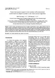
Figure 2 shows SEM image of coating surface. Here the flyash+ quartz+ illmenite composite powder is deposited on copper at 21 kW, 12 gm/min feed rate, 100mm torch to base distance with varying the power level. It is observed that surface contains some amount of pore with little surface roughness. In spraying the exact power level cannot be specified, because thermally sprayed coatings are very complex and incorporate process dependent defects such as splat gaps/interlamellar pores, globular pores, cracks (for ceramics), etc. It is clear that there is a close agreement of porosity measurement by the MFNN, LS-SVM and the experimental study, which indicates that the both the models can be used for predicting the amount coating porosity. Porosity formation by inter-splat position also depends on the mode of heat transfer through the substrate or prior deposited splats. This also similar to splat quenching by the Duwez gun technique. Inadequate amount of heat flow which results molten/semi-molten particles gather in a way to form more pore. Table 2. Variation of MSE (Etr) with Nh (η1=0.3, iteration = 400) h

1 2 3 4 5 6 7 8 9 10

Evaluation Criterion The Mean Square Error Etr for the training patterns after the mth iteration is defined as

 P 2  1  Etr    Vb1 p  Vb 2 p  m        p1  P

(4.16)

Where V1p is the experimental value of (Surface roughness in first case and Porosity of Plasma Sprayed Copper in second case), P is the number of training patterns and V2p (m) is the estimated value of (Surface roughness in first case and Porosity of Plasma Sprayed Copper in second case) after mth iteration. The training is stopped when the least value of Etr has been



= 0.6 and

Etr 4.2056× 10-5 6.0379 × 10-6 1.9029 × 10-6 9.9219 × 10-7 8.5546 × 10-7 5.8662 × 10-7 3.3196 × 10-7 1.9942 × 10-7 1.6227 × 10-7 1.4296 × 10-7

MFNN Modeling From Tables 2 and Figure 3, it is quite obvious that when Nh = 10,  = 0.6 and η1= 0.3, the MSE for training data is the lowest at 1.4296 × 10-7. The sequential mode of training has been adopted. It may be noted that the range of the values of η1 and  should be between 0 and 1and value of Nh should not more than 10 as per the HechtNielsen criteria. Hence we have stopped at Nh = 10 in Table1, we have stopped at η1= 0.3 and  = 0.6.

403

International Journal of Current Research, Vol. 4, Issue, 12, pp. 399-404, December, 2012

Fig. 3. Variation Mean Square Error (Etr) with number of iterations (η1=0.1,  = 0.6 and Nh=10) Fig. 1. Multilayer feed forward neural network LS-SVM Modeling From Figure 4, it is quite obvious that when  =0.31 , Sig2=5780.87 and iteration = 400, the data is well separated from LS-SVM hyper plane and mean square error (MSE) for training data is the lowest and equals to 7.15×10-7. It may be noted that if the value of iteration is increased MSE will decrease. Finally the test data are calculated by simply passing the input data in the LS-SVM and using  and b for the kernel parameter.

RESULT OBTAINED

Fig. 2. Surface morphology of plasma coated copper specimen (Spraying at 21KW power level).

Table 3 depicts the comparison between the MSE for the training data and testing data obtained from two different models using different techniques. As may be seen from Table-3 that LS-SVM model is better than MFNN model. This can be confirmed from the values of MSE.

Fig. 4. Shows the change of output parameter with respect to different input for training sample.

404

International Journal of Current Research, Vol. 4, Issue, 12, pp. 399-404, December, 2012

Table 3. Comparison of MSE for training & testing data of two models AC 270 300 400 420 270 300 400 420 270 300

V 40 50 45 50 40 50 45 50 40 50

PFR 12 12 12 12 15 15 15 15 18 18

PD 40 60 80 100 40 60 80 100 40 60

JSA 30 60 80 100 30 60 80 100 30 60

CT 300 350 290 280 315 360 300 290 320 340

ESR 14.33 12.4 12.4 14.06 14.01 13.8 13.9 14 14.5 13.8

AC- Arc current, V-Voltage, PFR- Powder Flow Rate, PDPowder size, JSA- Jet Spray Angle, CT-Coating Thickness, ESR- Experimental Surface roughness, EPPSR- Experimental Plasma Sprayed Copper, PSRN- Predicted Surface roughness using neural network, PPPSRN- Predicted Plasma Sprayed Copper using neural network, PSRS- Predicted Surface roughness using LSSVM, PPPSRS- Predicted Plasma Sprayed Copper using LSSVM. Conclusions In this study, a LS-SVM with RBF Kernel and feed forward neural network (MFNN) using Back Propagation algorithm was designed, trained and tested for prediction of surface roughness and porosity of plasma spray coating. The selected LS-SVM model successfully exhibited a good prediction capability with a low MSE for training and testing data than that of MFNN network. This can lead to reduce the time and cost of the process and improve the quality of the product.

REFERENCES [1] Satapathy Alok, Sahu Suvendu Prasad, Mishra Debadutta. 2010. Development of protective coatings using fly ash premixed with metal powder on aluminium substrates. Waste Management & Research. 28: 660-666. DOI: 10.1177/0734242X09348016 [2] Hetmanczyk M., Swadzba L., Mendala B. 2007. Advanced materials and protective coatings in aero-engines application. journal of Achievements in Materials and Manufacturing Engineering. vol. 24. Issue 1. 372-381. [3] Muggli P., Marsh K. A., Wang S., Clayton C. E., Lee S., T. C. Katsouleas, and Joshi C. 1999.Photo-Ionized Lithium Source for Plasma Accelerator Applications. IEEE Transactions On Plasma Science, vol. 27, no. 3, 1999, 791-799. [4] aBehera Ajit. 2012 Processing and Characterization of Plasma Spray Coatings of Industrial Waste and Low Grade Ore Mineral on Metal Substrates” Thesis Submitted For Master of Technology, Department of Metallurgical & Materials Engineering National Institute of Technology, Rourkela, India, 2012. [5] Ohtsu Y. 2012. Production of Low Electron Temperature Plasma and Coating of Carbon-Related Water-Repellent Films on Plastic Plate. IEEE Transactions on Plasma Science. Issue: 99, Page 1-6, DOI- 10.1109/TPS.2012.2194513 [6] Singla M. K., Singh Harpreet, ChawlaVikas. 2011. Thermal Sprayed CNT Reinforced Nanocomposite Coatings- A Review. Journal of Minerals & Materials Characterization &Engineering. Vol. 10. No.8. 717-726. [7] Davis J. R. 2004. Handbook of thermal spray technology in Thermal Spray Society Training Committee. Materials Park, OH: ASM Int, pp. 5. [8] Sampath S., Jiang X. 2001. Splat formation and microstructure development during plasma spraying: deposition temperature effects. Materials Science and Engineering: A, Vol. 304-306. 144–150.

EPPSR 22 28 23 18 24 26 21 20 28 27

PSRN 14.0206 12.5157 12.7141 13.7215 14.4761 13.9018 13.7836 13.8591 14.4925 13.6921

PPPSRN 21.6591 27.3736 21.4914 19.2354 23.8616 27.7279 21.4816 20.2544 26.7921 27.3341

PSRS 14.18 12.4 12.4 14.06 13.85 13.8 13.9 14 14.5 13.8

PPPSRS 21.93 27.843 22.62 17.642 24 26 21.326 20 27.89 27

[9] Zhang M., Wang X. and Luo J. 2011. Influence of Plasma Spraying on the Performance of Oxide Cathodes. IEEE transactions on electron devices. vol. 58, no. 7. 2143 -2148 [10] Heimann R. B. 2008. Plasma Spray Coating: Principles and Applications. New York: WILEY-VCH. pp. 81. [11] Fauchais P. 2004.Understanding plasma spraying. J. Phys. D: Appl. Phys. 37. 86-108. [12] bBehera Ajit, Mishra S.C. 2012. Prediction and analysis of Deposition Efficiency of Plasma Spray Coating using Artificial Intelligence Method. Open Journal of Composite Materials, 2. 54-60, doi:10.4236/ojcm.2012.22008. [13] Deshpande S., Kulkarni A., Sampath S., Herman H. 2004. Application of image analysis for characterization of porosity in thermal spray coatings and correlation with small angle neutron scattering. Surface & Coatings Technology. vol. 187. 6-16. [14] Vapnik V. N. 1995. Book: The Nature of Statistical Learning Theory”, Springer, New York. [15] Vapnik V. N. 1999. An Overview of Statistical Learning Theory. IEEE Transactions on Neural Networks, vol. 10, no. 5. 988-999. [16] Suykens J. A. K, Gestel T Van, Brabanter J De, Moor B De, Vandewalle J. 2002. Least Square SVM. World Scientific Pub. Co., Singapore. ISBN 981-238-151-1. [17] Hanbay D. 2009. An expert system based on least square support vector machines for diagnosis of the valvular heart disease. Expert Systems with Application. 36(4), part-1. 8368-8374. [18] Zuriani Mustaffa, Yuhanis Yusof. 2011. Optimizing LSSVM Using ABC For Non-Volatile Financial Prediction. Australian Journal of Basic and Applied Sciences, 5(11). 549-556. [19] Simon Haykin. 1999. Neural networks a comprehensive foundation. Prentice Hall International Inc, New Jersey, USA. 270-300,161-175. ISBN: 0023527617. [20] Hecht-Nielsen R. 1990. Neural network approach in scientific computing. Addison-Wesley Publishing Company Inc. 1990 433. [21] Ghosh S. and Kishore N. K. 1999. Modeling PD inception voltage of Epoxy Resin post insulators using an adaptive neural network. IEEE Transaction, Dielectrics and Electrical Insulation. Vol. 6. No. 1. 131-134. [22] Rumelhart D. E., Mcclelland J. L. (Eds.). 1986. Parallel distributed processing: explorations in the microstructure of cognition. MIT Press, vol. 1. 1986 - 567. [23] Simon Haykin. 1999. Neural networks a comprehensive foundation. Prentice Hall International Inc, New Jersey, USA. 161-175. [24] Mohanty S., Ghosh S. 2010. Artificial neural networks modeling of breakdown voltage of solid insulating materials in the presence of void. Institution of Engineering and Technology Science. Measurement and Technology. Vol. 4, Issue 58. 278-28. [25] Zegnini B., Mahdjoubi A. H. and Belkheiri M. 2011. A Least Squares Support Vector Machines (LS-SVM) Approach for Predicting Critical Flashover Voltage of Polluted Insulators. 2011 IEEE Conference on Electrical Insulation and Dielectric Phenomena, Mexico. 403-406.

*******