A Sparse Least Squares Support Vector Machine Classifier (Least squares support vector machines) József Valyon Gábor Horváth Department of Measurement and Information Systems Department of Measurement and Information Systems Budapest University of Technology and Economics Budapest University of Technology and Economics E-mail:
[email protected] E-mail:
[email protected]
Abstract – Since the early 90’s, Support Vector Machines (SVM) are attracting more and more attention due to their applicability to a large number of problems. To overcome the high computational complexity of traditional Support Vector Machines, recently a new technique, the Least–Squares SVM (LS–SVM) has been introduced, but unfortunately a very attractive feature of SVM, namely its sparseness, was lost. LS–SVM simplifies the required computation to solving linear equation set. This equation set embodies all available information about the learning process. By applying modifications to this equation set, we present a Least Squares version of the Least Squares Support Vector Machine (LS2–SVM). The proposed modification speeds up the calculations and provides better results, but most importantly it concludes a sparse solution. Introduction Among Neural Networks, the main advantage of SVM methods is that they automatically derive a network structure that guaranties an upper bound on the generalization error. This is very important in a large number of real life classification problems. Lately the Least–Squares Support Vector Machine (LS– SVM) is gaining more and more attention, mostly because it has some very attractive properties, regarding the implementation and the computational issues of teaching. In this case, training requires the solving a set of linear equations, instead of the quadratic programming problem involved by the standard SVM [1]. While the least squares version incorporates all training data in the network to produce the result, the traditional SVM selects a subset of them (called support vectors) including the samples that have a more significant effect on the classification. Because LS–SVM does not incorporate a support vector selection method, the resulting network size is usually much larger than it would be using the traditional SVM. This sparseness can also be reached with LS–SVM by applying a pruning method [2], but this iterative process requires an equation set –slowly decreasing in size–to be solved in every step, which multiplies the complexity. An optimal solution should combine the desirable features of these methods. It: (1)should be fast, (2)should lead to a sparse solution, (3)should produce good results. In order to achieve these goals, two new methods are introduced in the
sequel. The combination of these methods lead to a sparse, good quality LS–SVM solution, which means that a smaller network –based on a subset of the training samples– is accomplished, while all available information –training sample– is considered, all with the speed and simplicity of the least squares solution. The LS–SVM method is capable of solving both classification and regression problems. The present study concerns classification therefore only this is introduced in the sequel, along with the standard pruning method. Only a brief outline of these methods is presented, a detailed description can be found in refs. [2][3][4] and [5]. A brief overview of the LS–SVM method A. LS-SVM classification Given the
{xi ,di }iN=1
training data set, where x i ∈ ℜ p
represents a p–dimensional input vector with di ∈ {−1,+1} labels, our goal is to construct a classifier of form h y (x) = sign ∑ w jϕ j (x) + b = sign wT ϕ(x) + b , j =1 (1)
[
]
ϕ = [ϕ1 , ϕ 2 ,..., ϕ h ]T .
w = [ w1 , w2 ,..., wh ]T ,
The ϕ(.) : ℜ p → ℜ h is a mostly non-linear function, which maps the data into a higher (possibly infinite –h) dimensional feature space. The optimization problem can be given by the following equations ( k = 1,..., N ): min J p (w, e) = w ,b ,e
1 T 1 N w w + C ∑ ek2 2 2 k =1
[
(2)
]
with constraints: d k w T ϕ(x k ) + b = 1 − e k . The first term is responsible to find a smooth solution, while the second one minimizes the training errors ( C is the trade–off parameter between the terms). From this, the following Lagrangian can be formed: N
{ [
]
L(w, b, e;α) = J p (w, e) − ∑αk dk wT ϕ(xk ) + b −1+ ek k =1
}
(3)
, where the α k parameters are the Lagrange multipliers. The solution concludes in a constrained optimization with the conditions: ∂L =0 ∂w ∂L =0 ∂b ∂L =0 ∂ek ∂L =0 ∂α k
N
→ w = ∑ α k d k ϕ(x k ) →
k =1
N
∑αk dk = 0 k =1
→ α k = C ek
[
k = 1,..., N
(4)
]
→ d k w T ϕ(x k ) + b − 1 + ek = 0 k = 1,..., N
This can be formulated into the following linear equation set:
0 dT b 0 = r , −1 α + C d Ω I 1 d = [d1 , d 2 ,..., d N ]T , α = [α1,α2 ,..,αN ]T ,
(5)
r 1 = [1,...,1]T , Ω i , j = d i d j K (x i , x j ) .
where C ∈ ℜ is a positive constant, b is the bias and the result is: y (x) = ∑k =1 α k d k K (x, x k ) + b . This result can be N
interpreted as a neural network, which contains N non-linear neurons in its single hidden layer. The result ( y ) is the weighted sum of the outputs of the middle layer neurons. The weights are the calculated α k Lagrange multipliers. Although in practice SVMs are rarely formulated as actual networks, this neural interpretation is important, because it provides an easier discussion framework than the purely mathematical point of view. This paper uses the neural interpretation throughout the discussions, because the points and statements of this work can be more easily understood this way. The LS-SVM method –when RBF kernels are used– requires only two parameters ( C and σ), while the time consumed by the training method is reduced, by replacing the quadratic optimization problem with a simple linear equation set. One of the main drawbacks of the least–squares solution is that it is not sparse in the sense, that it incorporates all training vectors in the resulting network. In most real life situations the resulting networks are unnecessarily large. To overcome this problem, a pruning method was introduced. Pruning techniques are also well known in the context of traditional neural networks. Their purpose is to reduce the complexity of the networks by eliminating as much hidden neurons as possible. The method proposed later in this paper, not only results in a sparse model, it also has some positive effects concerning the algorithmic issues.
B. LS–SVM pruning Sparseness can also be reached with LS-SVM by applying a pruning method [2],[3], which eliminates some training samples based on the sorted support vector spectrum [2]. In the traditional SVM the result usually contains many zero weights. In the Least–Squares SVM the α k multipliers reflect the importance of the training points, since according to eq. 4, the α i weights are proportional to the ei errors in the training points: α i = Cei . By eliminating some vectors, represented by the smallest values from this α k spectrum, the number of neurons can be reduced. The irrelevant points are omitted, by iteratively leaving out the least significant vectors. These are the ones corresponding to the smallest α k values. The algorithm is the following [2]–[5]: 1. Train the LS–SVM based on N points. (N is the number of all available training vectors.) 2. Remove a small amount of points (e.g. 5% of the set) with the smallest values in the sorted α k spectrum. Re-train the LS–SVM based on the reduced training set. 4. Go to 2, unless the user–defined performance index degrades. If the performance becomes worse, it should be checked whether an additional modification of C, σ might improve the performance. In SVM sparseness is achieved by the use of such loss functions, where errors smaller than ε are ignored (ε– insensitive loss function). This method reduces the difference between the SVM and LS–SVM, because the omission of some data points implicitly corresponds to creating an ε– insensitive zone [4]. The described method leads to a sparse model, but some questions arise: How many neurons are needed in the final model? How many iterations it should take to reach the final model? Another problem is that a usually large linear system –slowly degrading in size- must be solved in all iteration. The pruning is especially important if the number of training vectors is large. In this case however, the iterative method is not very effective. This paper proposes a new method (the LS2–SVM), which leads to a sparse solution, automatically answers the questions and solves the problem described above. 3.
The proposed method C. Modifying the equation set If the training set consists of N samples, then our original linear equation set will have ( N + 1) unknowns, the α i -s,
( N + 1) equations and ( N + 1) 2 multiplication coefficients. These factors are the d j d k K k x j , x k kernel matrix elements
(
)
representing all training samples. The cardinality of the training set therefore determines the size of this coefficient matrix. Let’s take a closer look at the linear equation set describing the problem: 0 d T b 0 = r (6) −1 d Ω + C I α 1 where the first row means: N
∑α k dk = 0
(7)
k =1
and the j-th row stands for the: d j b + α1d j d1 K x j , x1 + ... + α k d j d k K x j , x k + C −1I + ... + α N d j d N
[ (
( ) K (x , x ) = 1 j
)
]
(8)
N
condition. To reduce the kernel matrix, columns and/or rows may be omitted. If the k–th column is left out, then the corresponding α k weight is also deleted, therefore the resulting will be sparser. If the k–th row is omitted, then the input–output defined by the (x k , d k ) training sample is lost. This leads to a less constrained, and therefore worst solution. When traditional iterative pruning is applied to the LS– SVM solution some training points are fully –from both column and row– omitted. These samples do not participate in the next kernel matrix, therefore information embodied in the subset of dropped points are entirely lost! Our proposition is to generalize the formulation of the kernel matrix. Reducing only the number of columns and not the rows means that the numbers of neurons are reduced, but all the known constraints are taken into consideration. This is the key concept of keeping the quality, while sparseness is achieved. The proposition presented here resembles to the basis of the Reduced Support Vector Machines (RSVM) introduced for standard SVM classification in ref. [6]. The RSVM selects a reduced training vector set ( M vectors) randomly and uses a reduced rectangular ( N × M ) kernel matrix, which reduces the size of the quadratic program to be solved. The number of kernels ( M ) may be less than N , so columns may be represented by M chosen c j vectors: {c1 , c 2 ,..., c M | c i ∈ {x1 , x 2 ,..., x N }, M < N } . (9) A possible method for selecting this subset of the samples is proposed in the next section. The formulation of Ω changes as follows: Ω j ,k = d j d k K x j , c k (10) The result will be calculated from:
(
)
y (x) = ∑ k =1 α k d k K (x, c k ) + b , where M is the number of M
kernels (nonlinear neurons) used.
Using fewer columns than training samples, means less weights ( αk ) and consequently a sparse solution. It also leads to an overdetermined equation set, which can be solved as a linear least–squares problem, consisting of only ( M + 1) × ( N + 1) coefficients.
0 dT 0 Ω + C−1 L Ω1,M b 1 1 , 1 M O M α1 M (11) = d L Ω j,M + C−1 M 1 Ω j,1 αM M M O M 1 L ΩN,1 ΩN,M This equation set is written shortly as Ax = b , where A , x and b are the matrixes in eq. (6) respectively. There is a slight problem with the regularisation parameter C since it can only be inserted in the first M rows, but it is enough to ensure us M linearly independent rows, so the equation set can be solved. The solution is calculated as (12) A T Ax = A T b The modified matrix A has ( N + 1) rows and ( M + 1) columns. After the matrix multiplications the results are obtained from a reduced equation set, incorporating AT A , which is only of size ( M + 1) × ( M + 1) . Since the modified LS–SVM equation set is solved in a least squares sense, we name this method LS2–SVM. D. A support vector selection method In the equation set, every variable (α k ) stands for a neuron, representing it’s output weighting. Each of the M selected training vectors will define a kernel function, therefore the selected samples must be evenly distributed and they should be of exactly the number required for a good solution. For the above described overdetermined solution, the following question must be answered: How many and which vectors are needed? Standard SVM automatically marks a subset of the training points as support vectors. In case of LS–SVM the linear equation set has to be reduced to an overdetermined equation set in such a way, that the solution of this reduced problem is the closest to what the original solution would be. As the matrix is formed from columns we can select a linearly independent subset of column vectors and omit all others, which can be formed as linear combinations of the selected ones. This can be done by finding a “basis” (the quote indicates, that this basis is only true under certain conditions defined later) of the coefficient matrix, because the basis is by definition the smallest set of vectors that can solve the problem. The slight modification of a common mathematical method can be utilized to find this “basis”. This method is used for bringing the matrix to the reduced row echelon form [7,8]. This is discussed in more detail in the sequel.
The basic idea of doing a feature selection in the kernel space is not new. The nonlinear principal component analysis technique, the Kernel PCA uses the same idea [9]. This reduced input set (the “support vectors”) is (are) selected automatically by determining a “basis” of the Ω (or the Ω + C −1I ) matrix. Let’s examine this a little closer! An Au = v linear equation set may be viewed as follows: if we consider the columns of A vectors, than v has to be the result of the weighted sum of these vectors. The equation set has a solution if and only if v is in the span of the columns of A. Every solution (u) means a possible decomposition of v to these vectors, but an LS–SVM problem requires only one(!). The solution is unique if and only if the columns of A are linearly independent. This means, that by determining a basis of A –any set of vectors, that are linearly independent, and span the same space as A– the problem can be reduced to a weighted sum of fewer vectors. In this proposed solution however, linear dependence does not mean exact linear dependence, because the method uses an adjustable tolerance value when determining the “resemblance” of the column vectors. The use of this tolerance value is essential, because none of the columns of Ω will likely be exactly dependent, especially if the selection is applied to the regularized Ω + C −1I matrix. This tolerance (ε’) can be related to the ε parameter of the standard SVM, because it has similar effects. The larger the tolerance, the fewer vectors the algorithm will select. If the tolerance is chosen too small, than a lot of vectors will seem to be independent, resulting in a larger network. As stated earlier the standard SVM’s sparseness is due to the ε– insensitive loss function, which allows the samples falling inside this insensitive zone to be neglected. It may not be very surprising to find, that an additional parameter is needed to achieve sparseness in LS–SVM. This parameter corresponds to ε, which was originally left when changing from the SVM to the standard least-squares solution. This selection process incorporates a parameter which indirectly controls the number of resulting basis vectors (M). This number does not really depend on the training sample number (N), but only on the problem, since M only depends on the number of linearly independent columns. In practice it means that if the problems complexity requires M neurons, than no matter how many training samples are presented, the size of the resulting network does not change. The reduction is achieved as a part of transforming the AT matrix into reduced row echelon form [7, 8]. The tolerance is used in the rank tests. The algorithm uses elementary row operations: 1. Interchange of two rows. 2. Multiply one row by a nonzero number. 3. Add a multiple of one row to a different row. The algorithm goes as follows [10]: 1. Loop over the entire matrix (i–row index, j– column index).
2.
Determine the largest element p in column j with row index i ≥ j. 3. If p ≤ ε’ (where ε’ is the tolerance) then zero out this part of the matrix (elements in the j–th row with index i ≥ j ); else remember the column index because we found a bases vector (support vector), and divide the row with the pivot element p and subtract the row from all other rows. 4. Step forward to i=i+1 and j=j+1. Go to step 1. This method returns a list of the column vectors which are linearly independent form the others considering tolerance ε’. The problem of choosing a proper ε’ resembles the selection of the other SVM hyper–parameters. One possibility is to use cross–validation, but as it will be seen later in the experiments, it is a trade–off problem between network size and performance. In the original LS-SVM pruning, the importance of a vector is considered to be proportional to the corresponding α k weight. In the light of the description above, it can be seen, that in every step this algorithm leaves out the “shortest” (least significantly weighted) vectors from the current decomposition of v . By doing this, the least important vectors are expected to be removed. Unfortunately this isn’t always true. If the number of training samples are very high, than it is unlikely to loose an important direction, but otherwise one may end up in a subspace of the original problem, because the resulting vector set do not span the original space. It is important to mention, that in the traditional algorithm, pruning means full reduction and therefore rows are also eliminated, which changes the vector space. Complexity issues This section discusses the algorithmic complexity of the described solutions. It is important to emphasize, that the primary goal of the described method is not an algorithmic gain, rather to achieve a sparse, and still precise solution,. LS–SVM training requires a linear equation set to be solved. In case of N training samples this can be solved by 1 using LU decomposition in N 3 + N 2 steps, each with one 3 multiplication and one addition [42]. If the training set comprises N points, than the equation set consists of N + 1 equations, that is the size of the matrix to be manipulated is ( N + 1) × ( N + 1) . As usually N >> 1 the effect of the one additional row can be neglected. Therefore to keep the formulas simple we will consider a matrix of size N × N . The reduced row echelon form of a matrix can be reached in N 2 steps. The proposed “support vector” selection is based on the result of this transformation. Let’s assume that the reduction leads to M selected vectors, and partial reduction
LS2-SVM
4
LS-SVM
6
NLS2-SVM
8
NLS-SVM
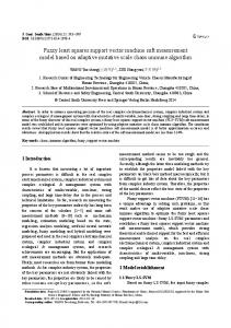
First, the two spiral benchmark problem is presented. The results for this CMU (Carnegie Melon University) benchmark is plotted on Fig. 1.. It shows that both methods are perfectly capable of distinguishing between the two input sets.
TABLE 1
NTS
Experiments
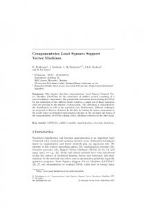
The next table summarizes the results for some UCI benchmarks. The results described here may not be the ones achieved for optimal hyper–parameter settings, but it is not that important in the comparison of LS–SVM and LS2–SVM. This is because by using 0 tolerance in the “reduced row” support vector selection method, the two methods are equivalent! Of course, in the experiments we were aiming at using nearly optimal hyper parameter settings. NTR is the number of training inputs and NTS is the number of test samples. The column marked NLS2-SVM contains the network size of our sparse solution. The last two columns show the hit/miss classification rates for the test sets. In the experiments we split the datasets to a training and test set as seen in ref. [5] .
NTR
is used. In this case, the calculation of A T A (defined in eq. 17.) requires M 2 N steps. Solving this new equation set costs 1 3 M + M 2 steps. The total cost of the proposed of 3 1 algorithm adds up to: N 2 + M 2 N + M 3 + M 2 . If 3 M