EE263 Autumn 2007-08. Stephen Boyd. Lecture 7. Regularized least-squares
and Gauss-Newton method. • multi-objective least-squares. • regularized least- ...
EE263 Autumn 2007-08
Stephen Boyd
Lecture 7 Regularized least-squares and Gauss-Newton method • multi-objective least-squares • regularized least-squares • nonlinear least-squares • Gauss-Newton method
7–1
Multi-objective least-squares in many problems we have two (or more) objectives • we want J1 = kAx − yk2 small • and also J2 = kF x − gk2 small (x ∈ Rn is the variable) • usually the objectives are competing • we can make one smaller, at the expense of making the other larger common example: F = I, g = 0; we want kAx − yk small, with small x Regularized least-squares and Gauss-Newton method
7–2
Plot of achievable objective pairs plot (J2, J1) for every x:
J1
x(1) x(2)
x(3)
J2 note that x ∈ Rn, �but this plot is in R2; point labeled x(1) is really J2(x(1)), J1(x(1)) Regularized least-squares and Gauss-Newton method
7–3
• shaded area shows (J2, J1) achieved by some x ∈ Rn • clear area shows (J2, J1) not achieved by any x ∈ Rn • boundary of region is called optimal trade-off curve • corresponding x are called Pareto optimal (for the two objectives kAx − yk2, kF x − gk2)
three example choices of x: x(1), x(2), x(3) • x(3) is worse than x(2) on both counts (J2 and J1) • x(1) is better than x(2) in J2, but worse in J1
Regularized least-squares and Gauss-Newton method
7–4
Weighted-sum objective
• to find Pareto optimal points, i.e., x’s on optimal trade-off curve, we minimize weighted-sum objective J1 + µJ2 = kAx − yk2 + µkF x − gk2 • parameter µ ≥ 0 gives relative weight between J1 and J2 • points where weighted sum is constant, J1 + µJ2 = α, correspond to line with slope −µ on (J2, J1) plot
Regularized least-squares and Gauss-Newton method
7–5
PSfrag
J1
x(1) x(3) x(2) J1 + µJ2 = α J2
• x(2) minimizes weighted-sum objective for µ shown • by varying µ from 0 to +∞, can sweep out entire optimal tradeoff curve
Regularized least-squares and Gauss-Newton method
7–6
Minimizing weighted-sum objective can express weighted-sum objective as ordinary least-squares objective:
� � � � 2
A y
= √ x− √ µF µg
2
˜
= Ax − y˜
kAx − yk2 + µkF x − gk2
where A˜ =
�
A √ µF
�
,
y˜ =
�
y √ µg
�
hence solution is (assuming A˜ full rank) x = =
�
�−1 A A˜ A˜T y˜ ˜T T
T
A A + µF F
Regularized least-squares and Gauss-Newton method
�−1
T
T
A y + µF g
� 7–7
Example f
• unit mass at rest subject to forces xi for i − 1 < t ≤ i, i = 1, . . . , 10 • y ∈ R is position at t = 10; y = aT x where a ∈ R10 • J1 = (y − 1)2 (final position error squared) • J2 = kxk2 (sum of squares of forces) weighted-sum objective: (aT x − 1)2 + µkxk2 optimal x: T
x = aa + µI Regularized least-squares and Gauss-Newton method
�−1
a 7–8
optimal trade-off curve: 1
0.9
0.8
J1 = (y − 1)2
0.7
0.6
0.5
0.4
0.3
0.2
0.1
0
0
0.5
1
1.5
2
J2 = kxk2
2.5
3
3.5 −3
x 10
• upper left corner of optimal trade-off curve corresponds to x = 0 • bottom right corresponds to input that yields y = 1, i.e., J1 = 0 Regularized least-squares and Gauss-Newton method
7–9
Regularized least-squares when F = I, g = 0 the objectives are J1 = kAx − yk2,
J2 = kxk2
minimizer of weighted-sum objective, T
x = A A + µI
�−1
AT y,
is called regularized least-squares (approximate) solution of Ax ≈ y • also called Tychonov regularization • for µ > 0, works for any A (no restrictions on shape, rank . . . ) Regularized least-squares and Gauss-Newton method
7–10
estimation/inversion application: • Ax − y is sensor residual • prior information: x small • or, model only accurate for x small • regularized solution trades off sensor fit, size of x
Regularized least-squares and Gauss-Newton method
7–11
Nonlinear least-squares
nonlinear least-squares (NLLS) problem: find x ∈ Rn that minimizes kr(x)k2 =
m X
ri(x)2,
i=1
where r : Rn → Rm • r(x) is a vector of ‘residuals’ • reduces to (linear) least-squares if r(x) = Ax − y
Regularized least-squares and Gauss-Newton method
7–12
Position estimation from ranges estimate position x ∈ R2 from approximate distances to beacons at locations b1, . . . , bm ∈ R2 without linearizing
• we measure ρi = kx − bik + vi (vi is range error, unknown but assumed small) • NLLS estimate: choose x ˆ to minimize m X
ri(x)2 =
i=1
Regularized least-squares and Gauss-Newton method
m X i=1
2
(ρi − kx − bik)
7–13
Gauss-Newton method for NLLS
NLLS: find x ∈ Rn that minimizes kr(x)k2 = n
r:R →R
m
m X
ri(x)2, where
i=1
• in general, very hard to solve exactly • many good heuristics to compute locally optimal solution Gauss-Newton method: given starting guess for x repeat linearize r near current guess new guess is linear LS solution, using linearized r until convergence Regularized least-squares and Gauss-Newton method
7–14
Gauss-Newton method (more detail): • linearize r near current iterate x(k): r(x) ≈ r(x(k)) + Dr(x(k))(x − x(k)) where Dr is the Jacobian: (Dr)ij = ∂ri/∂xj • write linearized approximation as r(x(k)) + Dr(x(k))(x − x(k)) = A(k)x − b(k) A(k) = Dr(x(k)),
b(k) = Dr(x(k))x(k) − r(x(k))
• at kth iteration, we approximate NLLS problem by linear LS problem:
2
(k) (k) kr(x)k ≈ A x − b 2
Regularized least-squares and Gauss-Newton method
7–15
• next iterate solves this linearized LS problem: (k+1)
x
�
= A
(k)T
A
(k)
�−1
A(k)T b(k)
• repeat until convergence (which isn’t guaranteed)
Regularized least-squares and Gauss-Newton method
7–16
Gauss-Newton example • 10 beacons • + true position (−3.6, 3.2); ♦ initial guess (1.2, −1.2) • range estimates accurate to ±0.5 5
4
3
2
1
0
−1
−2
−3
−4
−5 −5
−4
−3
−2
Regularized least-squares and Gauss-Newton method
−1
0
1
2
3
4
5
7–17
NLLS objective kr(x)k2 versus x: 16
14
12
10
8
6
4
2 5 0 5
0 0 −5
−5
• for a linear LS problem, objective would be nice quadratic ‘bowl’ • bumps in objective due to strong nonlinearity of r Regularized least-squares and Gauss-Newton method
7–18
objective of Gauss-Newton iterates: 12
10
kr(x)k2
8
6
4
2
0
1
2
3
4
5
6
7
8
9
10
iteration • x(k) converges to (in this case, global) minimum of kr(x)k2 • convergence takes only five or so steps Regularized least-squares and Gauss-Newton method
7–19
• final estimate is x ˆ = (−3.3, 3.3) • estimation error is kˆ x − xk = 0.31 (substantially smaller than range accuracy!)
Regularized least-squares and Gauss-Newton method
7–20
convergence of Gauss-Newton iterates: 5 4 3
4 56 3
2 2
1
0
1
−1
−2
−3
−4
−5 −5
−4
−3
−2
Regularized least-squares and Gauss-Newton method
−1
0
1
2
3
4
5
7–21
useful varation on Gauss-Newton: add regularization term kA(k)x − b(k)k2 + µkx − x(k)k2 so that next iterate is not too far from previous one (hence, linearized model still pretty accurate)
Regularized least-squares and Gauss-Newton method
7–22