Lectures in Dynamic Programming and Stochastic Control - Stanford ...

Lectures in Dynamic Programming and Stochastic Control Arthur F. Veinott, Jr.

Spring 2008 MS&E 351 Dynamic Programming and Stochastic Control

Department of Management Science and Engineering Stanford University Stanford, California 94305

Copyright © 2008 by Arthur F. Veinott, Jr.

Contents 1 Discrete-Time-Parameter Finite Markov Population Decision Chains...................................1 1 FORMULATION................................................................................................................................. 1 2 MAXIMUM R -PERIOD VALUE: RECURSION AND EXAMPLES................................................ 3 Minimum-Cost Chain........................................................................................................................4 Supply Management......................................................................................................................... 5 Exercising a Call Option...................................................................................................................6 System Reliability............................................................................................................................. 7 Maximum Expected R -Period Instantaneous Rate of Return: Portfolio Selection.......................... 8 3 MAXIMUM EXPECTED R -PERIOD UTILITY WITH CONSTANT RISK POSTURE................ 9 Expected Utilities and Risk Aversion/Preference............................................................................. 9 Constant Additive Risk Posture..................................................................................................... 10 Constant Multiplicative Risk Posture.............................................................................................11 Additive and Multiplicative Utility Functions................................................................................11 Maximum Expected R -Period Symmetric Multiplicative Utility................................................... 12 Maximum R -Period Instantaneous Rate of Expected Return........................................................12 4 MAXIMUM VALUE IN CIRCUITLESS SYSTEMS.........................................................................12 Knapsack Problem (Capital Budgeting)......................................................................................... 13 Portfolio Selection........................................................................................................................... 14 5 DECISIONS, POLICIES, OPTIMAL-RETURN OPERATOR.........................................................14 6 MAXIMUM R -PERIOD VALUE: FORMALITIES..........................................................................15 Advantages of Maximum-R -Period-Value Policies.........................................................................16 Rolling Horizons and the Backward and Forward Recursions........................................................16 Limitations of Maximum-R -Period-Value Policies......................................................................... 17 7 MAXIMUM VALUE IN TRANSIENT SYSTEMS............................................................................17 Why Study Infinite-Horizon Problem............................................................................................. 17 Characterization of Transient Matrices.......................................................................................... 18 Transient System............................................................................................................................ 19 Comparison Lemma........................................................................................................................ 19 Policy-Improvement Method...........................................................................................................20 Stationary Maximum-Value Policies: Existence and Characterization...........................................21 Newton’s Method: A Specialization of Policy-Improvement Method............................................. 22 Successive Approximations: Maximum R -Period Value Converges to Maximum Value............... 22 Geometric Interpretation: a Single-State Reliability Example........................................................23 System Degree, Spectral Radius and Polynomial Boundedness......................................................24 Geometric Convergence of Successive Approximations.................................................................. 27 Contraction Mappings.....................................................................................................................28 Linear-Programming Method.......................................................................................................... 29 State-Action Frequency...................................................................................................................31 Simplex Method: A Specialization of Policy-Improvement Method............................................... 34 Running Times................................................................................................................................35 Stochastic Constraints.....................................................................................................................37 Stationary Randomized Policies......................................................................................................37 Supply Management with Service Constraints............................................................................... 39 Maximum Present Value.................................................................................................................39 Multi-Armed Bandit Problem: Optimality of Largest-Index Rule..................................................41

i

MS&E 351 Dynamic Programming Copyright © 2008 by Arthur F. Veinott, Jr.

ii

Contents

8 MAXIMUM PRESENT VALUE WITH SMALL INTEREST RATES IN BOUNDED SYSTEMS.... 45 Bounded System..............................................................................................................................46 Strong Maximum Present Value in Bounded Systems................................................................... 46 Cesàro Limits and Neumann Series................................................................................................ 46 Stationary and Deviation Matrices................................................................................................. 47 Laurent Expansion of Resolvent..................................................................................................... 49 Laurent Expansion of Present Value for Small Interest Rates....................................................... 50 Characterization of Stationary Strong Maximum-Present-Value Policies...................................... 50 Application to Controlling Service and Rework Rates in a G/M/_ Queue.................................. 51 Strong Policy-Improvement Method............................................................................................... 53 Existence and Characterization of Stationary Strong Maximum-Present-Value Policies...............54 Truncation of Infinite Matrices....................................................................................................... 55 8-Optimality: Efficient Implementation of the Strong Policy-Improvement Method.....................57 9 CESÀRO OVERTAKING OPTIMALITY WITH IMMIGRATION IN BOUNDED SYSTEMS.....60 Controlled Queueing Network with Proportional Service Rates.....................................................61 Cash Management...........................................................................................................................62 Manpower Planning........................................................................................................................ 62 Insurance Management................................................................................................................... 62 Asset Management.......................................................................................................................... 63 Immigration Stream........................................................................................................................ 63 Cohort and Markov Policies............................................................................................................63 Overtaking Optimality.................................................................................................................... 65 Cesàro Overtaking Optimality........................................................................................................ 66 Convolutions................................................................................................................................... 66 Binomial Coefficients and Sequences.............................................................................................. 67 Polynomial Expansion of Expected Population Sizes with Binomial Immigration........................ 68 Polynomial Expansion of R -Period Values.....................................................................................70 Comparison Lemma for R -Period Values....................................................................................... 72 Cesàro Overtaking Optimality with Binomial Immigration Stream...............................................73 Reward-Rate Optimality.................................................................................................................73 Cesàro Overtaking Optimality........................................................................................................ 74 Float Optimality............................................................................................................................. 74 Value Interpretation of Immigration Stream.................................................................................. 75 Combining Physical and Value Immigration Streams.................................................................... 75 Cesàro Overtaking Optimality with More General Immigration Streams...................................... 76 Future-Value Optimality................................................................................................................ 78 10 SUMMARY.......................................................................................................................................78

2 Team Decisions, Certainty Equivalents and Stochastic Programming.................................81 1 FORMULATION AND EXAMPLES................................................................................................ 81 Airline Reservations with Uncertain Demand.................................................................................82 Inventory Control with Uncertain Demand.................................................................................... 83 Transportation Problem with Uncertain Demand.......................................................................... 84 Capacity Planning with Uncertain Demand................................................................................... 84 2 REDUCTION OF STOCHASTIC TO ORDINARY MATHEMATICAL PROGRAMS..................85 Linear and Quadratic Programs......................................................................................................86 Computations.................................................................................................................................. 87 Comparison of Dynamic and Stochastic Programming.................................................................. 87


iii

Contents

3 QUADRATIC UNCONSTRAINED TEAM DECISION PROBLEMS............................................. 88 4 SEQUENTIAL QUADRATIC UNCONSTRAINED TEAMS: CERTAINTY EQUIVALENTS...... 89 Interpretation of Solution................................................................................................................90 Computations.................................................................................................................................. 90 Quadratic Control Problem............................................................................................................ 91 Rocket Control................................................................................................................................ 91 Multiproduct Supply Management................................................................................................. 91 Dynamic Programming Solution with Zero Random Errors...........................................................92 Solution with Independent Random Errors.................................................................................... 94 Solution with Dependent Random Errors.......................................................................................94 Strengths and Weaknesses.............................................................................................................. 95

3 Continuous-Time-Parameter Markov Population Decision Processes..................................97 1 FINITE CHAINS: FORMULATION................................................................................................. 97 2 MAXIMUM X -PERIOD VALUE: BELLMAN’S EQUATION AND EXAMPLES...........................98 Controlled Queues...........................................................................................................................99 Supply Management........................................................................................................................99 Project Scheduling...........................................................................................................................99 3 PIECEWISE-CONSTANT POLICIES, GENERATORS, TRANSITION MATRICES................. 100 Nonnegative, Substochastic and Stochastic Transition Matrices..................................................101 4 CHARACTERIZATION OF MAXIMUM X -PERIOD-VALUE POLICIES................................... 101 5 EXISTENCE OF MAXIMUM X -PERIOD-VALUE POLICIES..................................................... 103 6 MAXIMUM X -PERIOD VALUE WITH A SINGLE STATE.........................................................106 7 EQUIVALENCE PRINCIPLE FOR INFINITE-HORIZON PROBLEMS......................................108 8 MAXIMUM PRINCIPLE................................................................................................................. 110 Linear Control Problem................................................................................................................ 112 Markov Population Decision Chain.............................................................................................. 113 9 MAXIMUM PRESENT VALUE FOR CONTROLLED ONE-DIMENSIONAL DIFFUSIONS.....113 Diffusions.......................................................................................................................................113 Probability of Reaching One Boundary Before the Other............................................................ 116 Mean Time to Reach Boundary.................................................................................................... 117 Controlled Diffusions.....................................................................................................................117 Maximizing the Probability of Accumulating Given Wealth........................................................118

Appendix: Functions of Matrices............................................................................................. 121 1 2 3 4 5 6 7 8

MATRIX NORM.............................................................................................................................. 121 EIGENVALUES AND VECTORS...................................................................................................122 SIMILARITY....................................................................................................................................122 JORDAN FORM.............................................................................................................................. 122 SPECTRAL MAPPING THEOREM...............................................................................................123 MATRIX DERIVATIVES AND INTEGRALS............................................................................... 124 MATRIX EXPONENTIALS............................................................................................................ 125 MATRIX DIFFERENTIAL EQUATIONS...................................................................................... 125

References................................................................................................................................. 127 BOOKS................................................................................................................................................ 127 SURVEYS............................................................................................................................................128 ARTICLES.......................................................................................................................................... 128

Index of Symbols.................................................................................................................................... 131


iv

Contents

Homework Assignments Homework 1 (4/11/08) Exercising a Put Option Requisition Processing Matrix Products Bridge Clearance

Homework 2 (4/18/08) Dynamic Portfolio Selection with Constant Multiplicative Risk Posture Airline Overbooking Sequencing: Optimality of Index Policies

Homework 3 (4/25/08) Multifacility Linear-Cost Production Planning Discovering System Transience Successive Approximations and Newton’s Method Find Nearly Optimal Policies in Linear Time

Homework 4 (5/2/08) Component Replacement Optimal Stopping Policy Simple Stopping Problems House Buying

Homework 5 (5/9/08) Bayesian Statistical Quality Control and Repair Minimum Expected Present Value of Sojourn Times Optimal Control of Tandem Queues

Homework 6 (5/16/08) Limiting Present-Value Optimality with Binomial Immigration Maximizing Reward Rate by Linear Programming

Homework 7 (5/23/08) Discovering System Boundedness Finding the Maximum Spectral Radius Irreducible Systems and Cesàro-Geometric-Overtaking Optimality

Homework 8 (5/30/08) Element-Wise Product of Symmetric Positive Semi-Definite Matrices Quadratic Unconstrained Team-Decision Problem with Normally Distributed Observations Optimal Baking

Homework 9 (6/4/08) Pricing a House for Sale Transient Systems in Continuous Time

1 Discrete-Time-Parameter Finite Markov Population Decision Chains 1 FORMULATION A discrete-time-parameter finite Markov population decision chain is a system that involves a finite population evolving over a sequence of periods labeled "ß #ß á . and over which one can exert some control. The system description depends on four data elements, viz., states, actions, rewards and transition rates. In each period R , each individual is in some state = in a set f of W  _ states. The state summarizes all “relevant” information about the system history L as of period R . Each individual in state = chooses an action + from a finite set E=L œ E= of possible actions, earns a reward l =ß +Ñ ! of individuals in state > − f in period R ". Call :Ð> l =ß +Ñ the transition rate. The assumptions that E, < and : depend on L only through = are essential for a state = in a period to summarize all relevant information about the system history L as of the period. Ob-

1For

nearly all optimality concepts considered in the sequel, it suffices to consider only the expected numbers of individuals entering each state rather than the distribution of the actual random numbers of individuals entering each state. For that reason, those distributions are not considered explicitly here.

1


2

§1 Discrete Time Parameter

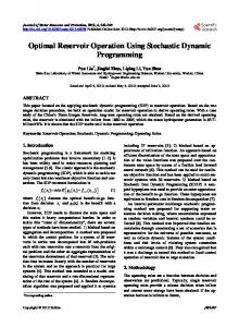
serve that the size of the population may vary over time. Also, there is no interaction among the individuals. Figure 1 illustrates this situation.

ã =

+

:

> ã

Figure 1

Call a system stochastic (resp., substochastic) if !> :Ð> l =ß +Ñ œ " (resp., Ÿ ") for each + − E= and = − f . An important instance of a stochastic (resp., substochastic) system is that in which

:Ð> l =ß +Ñ is the probability that an individual in state = who takes action + in a period generates a single individual in state >.2 Call a stochastic system deterministic if the :Ð> l =ß +Ñ are all ! or " because then for each = and + there will be a unique > − f for which :Ð> l =ß +Ñ œ " and :Ð7 l =ß +Ñ

œ ! for all 7 Á >. Examples of States and Actions in Various Applications. The table below gives examples of states and actions in several application areas. Application Manage supply chain Maintain road Invest in securities Inspect lot Route calls Control queueing network Overbook flight Market product Manage reservoirs Insure asset Patrol area Guide rocket Care for a patient

State Inventory levels of products Condition of road Portfolio of securities Number of defectives Nodes in network Queue sizes at each station Number of reservations Goodwill Water levels at reservoirs Risk category Car locations, service requests Position and velocity Condition of patient

Action Choose product order times/quantities Select resurfacing option Buy/sell securities: times and amounts Accept/reject lot, continue sampling Send a call at one node to another Set service rates at each station Book/decline reservation request Advertise product Release water from reservoirs Set policy premium Reposition cars Choose retrorockets to fire Conduct tests and treatments

In practice, it is often the case that the reward l =ß +ÑZ>R " . >−f

reward in first period

expected reward in remaining R " periods when an optimal policy is used therein

Moreover, if the individual chooses an “optimal” action + in the first period, then equality occurs above. This idea, called the principle of optimality, implies the dynamic-programming recursion: (1)

Z=R œ max Ò−f


4


for = − f and R œ "ß #ß á ß where Z=! is the given terminal value in state =. This recursion permits one to calculate ÖZ=" ×, then ÖZ=# ×, then ÖZ=$ ×, and so on. Once Z=R is computed, one optimal action +R = in state = with R periods to go is simply any action in E= that achieves the maximum on the right-hand side of (1). Thus, when there are R periods to go, each individual in state = can be assumed to take the same action without loss of optimality. The recursion Ð1) is of fundamental importance in a broad class of applications. Minimum R -Period Cost. If . In that event, it is best to choose one with maximum reward and eliminate the others. Then one can identify actions in state = with states > visited next, so (1) simplifies to

Z=R œ max ÒÑ  Z>R " Ó

(2)

>−E=

for = − f and R œ "ß #ß á . As Figure 2 illustrates, Z=R can be thought of as the maximum R -period reward that an individual can earn in traversing an R -step chain that begins in state = and earns a terminal reward Z>! when it ends in state >.

Z =R

= > N

N1

N2

1

Z >!

0

Figure 2 Examples 1 Minimum-Cost Chain. The minimum-cost-chain problem described above has a terminal cost in each state. One specialization of this problem is to find a minimum-cost chain from every state to a given terminal state 7 in R steps or less. Thus if -Ð=ß >Ñ is the cost of moving from state = to state > in one step and G=R is the minimum R -step-or-less cost of moving from state = to state 7 ,

then G7R œ ! for R ", G=" œ -Ð=ß 7 Ñ and (3)

G=R œ min Ò-Ð=ß >Ñ  G>R " Ó, R œ #ß $ß á and = − f Ï Ö7 ×. >−E=


5


If the associated (directed) graph Z ´ Ðf ß TÑ with node set f and arc set T ´ ÖÐ=ß >Ñ À > − E= × has

no circuit (i.e., directed cycle) around which the total cost incurred is negative, then G=R œ G=W" for = − f Ï Ö7 × and R W  ".

(4)

This is because a minimum-cost chain from = to 7 need not visit a node twice. For if it did, the chain could be shortened and its cost reduced by eliminating the circuit created by visiting the indicated node twice as Figure 3 illustrates. Thus a minimum-cost chain from any node in f Ï Ö7 × to 7 can be assumed to have W  " arcs or less, justifying (4). If one takes care to choose the minR R " imizer > œ >R whenever G=R œ G=R " , then the >R = in (3) so that >= œ >= = œ >= will be independ-

ent of R W  " by (4). Also, the subgraph of Z with arcs Ð=ß >= Ñ, = − f Ï Ö7 ×, is a tree with the unique simple chain therein from each node = Á 7 to 7 being a minimum-cost chain from = to 7 .

2 1 =

6 3

2

7

5

6

7

1 =

4 Figure 3

Computational Effort (or Complexity). How much computation is required to calculate G= ´ G=W"

for all = − f Ï Ö7 ×? Let E be the number of arcs in T. Then for each R , evaluation of (3) re-

quires E additions and nearly the same number of comparisons. Since this must be done for each R œ #ß á ß W", the total number of additions and comparisons is about ÐW  #ÑE. 2 Supply Management. One of the areas in which dynamic programming has been used most

widely is to find optimal supply-management policies. The reason for this is that nearly all firms carry inventories and the investment in them is sizable. For example, US manufacturing and trade inventories alone in 2000 were 1.205 trillion dollars, or 12% of the entire US gross national product of 9.963 trillion dollars that year!3 As an illustration of the role of dynamic programming in such problems, suppose that the de-

mands for a single product in successive periods are independent and identically-distributed random variables. At the beginning of a period, the supply manager observes the initial stock =, ! Ÿ =

Ÿ W , and orders a nonnegative amount with immediate delivery bringing the starting stock to +, = Ÿ + Ÿ W . If the demand H in the period exceeds +, the excess demand H  + is lost. There is an ordering cost -Ð+  =Ñ and a holding and penalty cost 2Ð+  HÑ in the period. Let G=R be the minimum expected R -period cost starting with the initial stock =. Then ÐG†! ´ !Ñ

32001

Statistical Abstract of the United States, Table 756 and 640.


6


R " G=R œ min Ò-Ð+  =Ñ  E2Ð+  HÑ  EGÐ+HÑ Ó =Ÿ+ŸW

for ! Ÿ = Ÿ W and R œ "ß #ß á . 3 Exercising a Call Option. One of the most active places in which dynamic programming is

used today is Wall Street. To illustrate, consider the problem of determining when to exercise an (American) call option to buy a stock ignoring commissions. The option gives the purchaser the right to buy the stock at the strike price =‡ ! on any of the next R days. Two questions arise. When should the option be exercised? What is its value? To answer these questions requires a stock-price model and a dynamic-programming recursion to find the value of the option as well as an optimal option-exercise policy.4 Consider the following stock-price model. Suppose that the stock price is = on day R !, i.e., R days before the option expires. If R  !, assume that the stock price on the following day R " is =VR where V" ß V# ß á are independent identically distributed nonnegative random variables with the same distribution as a nonnegative random variable V. Then, < ´ V  " is the rate

of return for a day, and E< is the expected rate of return that day. Let Z=R be the value of the option on day R when the market price of the stock is =. There are two alternatives that day. One is to exercise the option to buy the stock at the strike price and immediately resell it, which earns =  =‡ . The other is not to exercise the option that day, in R " which case the maximum expected income in the remaining R " days is EZ=V . Since one seeks

the alternative with higher expected future income, the value of the option on expiration day is

Z=! œ Ð=  =‡ Ñ and on day R  ! is given recursively by (5)

R " Z=R œ maxÐ=  =‡ ß EZ=V Ñß R œ "ß #ß á .

Thus it is optimal to exercise the option on expiration day if =  =‡  !, and not do so otherwise. R" And it is optimal to exercise the option on day R  ! if =  =‡  EZ=V , and not do so otherwise.

Nonnegative Expected Rate of Return. Consider now the question when it is optimal to

exercise the option. It turns out that as long as the expected rate of return is nonnegative, i.e., E< ! or equivalently EV ", the answer is to wait until the expiration day. To establish this fact, it suffices to show that (6) 4This

R " Z=R œ EZ=V

formulation of the problem of when to exercise an (American) call option addresses the situation faced by an investor who wishes to profit from speculation on the market price of a stock. By contrast, the formulation of the problem in finance addresses the problem faced by an institution who wishes to price an option to avoid market risk and rely on commissions for profits. Though the assumptions differ, the computations are similar.


7


for each R  ! and all = !. To that end, observe from (5) for R  " and by definition for R œ R " " that Z=R " =  =‡ for each = !. Thus because EV ", it follows that EZ=V EÐ=V  =‡ Ñ

=  =‡ . Hence from (5) again, (6) holds. Hence, if the expected rate of return is nonnegative, it is optimal not to exercise the option at any market price when R  ! days remain until expiration. R Furthermore, Z=R œ EÐ=VR  =‡ Ñ is the value of the option where V R ´ #R is the " V3 , so =V

price at expiration. Negative Expected Rate of Return. Suppose now that the expected rate of return is nega-

tive, i.e., E<  !. To analyze equation (5), it turns out to be useful to subtract =  =‡ from both sides of (5) and make the change of variables Y=R œ Z=R  Ð=  =‡ Ñ. Then (5) reduces to the equiv-

alent system (5)w

R " Y=R œ maxÐ!ß =E<  EY=V Ñ

for R œ "ß #ß á where Y=! œ Ð=‡  =Ñ . Now we claim that Y=R is decreasing and continuous in = ! for each R and lim=Ä_ Y=R œ !. Certainly that is so for R œ !. Suppose it is so for R " R " and consider R . Then EY=V is decreasing and continuous in = and approaches ! as = Ä _. R " Consequently, there is a smallest = œ =R ! such that =E<  EY=V Ÿ !. Thus, it follows that R " the maximum on the right side of (5)w is =E<  EY=V if =  =R and ! if = =R . Since (5) and

(5)w are equivalent, it follows that this rule is optimal with (5) as well, i.e., it is optimal to wait if =  =R and to exercise the option if = =R . In short, if the expected rate of return is negative and if R days remain until expiration of the option, then there is a price limit =R such that it is optimal to wait if the price is below =R and to exercise the option if the price is =R or higher. 4 System Reliability. A system consists of a finite set D of components. The system is ob-

served once a period and each component is found to be “working” or “failed.” If = is the subset of components that is observed to be working in some period, then a subset > Ï = of the failed com-

ponents may be replaced at a cost Ï= where > Ð ª =Ñ is the set of working components after replacement. The expected operating cost incurred during the period is then :> . Some components may fail during the period with the conditional distribution of the random set A of working com-

ponents in the next period, given that > is the working set after replacement in the period and given the past history, depending on >, but not otherwise on the past history. Let G=R be the minimum expected R -period cost when = is the initial working set. Then ÐG†! ´ !Ñ, G=R œ min ÒÏ=  :>  EÐGAR " l >ÑÓ =©>©D

for g © = © D and R œ "ß #ß á .


8


5 Maximum Expected R -Period Instantaneous Rate of Return: Portfolio Selection. Sup-

pose that in a stochastic system, the return the system earns in periods "ß á ß R is the product V" â VR of the nonnegative random returns V" ß á ß VR in those periods. For example, if the rate of return in period 3 is 15%, then the return in period 3 is V3 œ 1.15. Now let 1003R % be the (random) instantaneous rate of return per period over the R periods assuming continuous compounding. Then /3R R œ V" â VR , so (7)

3R œ

" ÒlnV"  â  lnVR Ó. R

Now since lnV3 is the instantaneous rates of return in period 3, the problem of maximizing the expected instantaneous rate of return over R periods reduces to maximizing the sum E lnV"  â  E lnVR of the expected instantaneous rates of return in those R periods. Now assume that the conditional distribution of V3 given that the system starts in state = in

period 3 and takes action + − E= in that period, and given the past history, is independent of 3 and of the past history. Then the corresponding conditional expected value l =ß +Ñ œ :Ð> l =Ñ. Let Z=R be the maximum expected value

of the instantaneous rate of return over R periods when the market state is initially =. Then (1) holds with :Ð> l =Ñ replacing :Ð> l =ß +Ñ. Consequently, since an action in E= maximizes the righthand side of (1) if and only if it maximizes :Ð> l =ÑZ>R" is independent of +. This means that the optimal policy is myopic, i.e., maximizes the (expected) reward in each period alone without regard for the future. Thus, in the present case, it suffices to separately maximize the expected instantaneous rate of return in each period. 3 MAXIMUM EXPECTED R -PERIOD UTILITY WITH CONSTANT RISK POSTURE

[HM72], [Ar65], [Ro75a] Expected Utility and Risk Aversion/Preference Expected Utility. A decision maker’s preferences among gambles, which we take to be

random R -vectors, can often be expressed by a utility function, i.e., a real-valued function ? defined on the range (assumed in d R ) of the set of gambles. When this is so, a decision maker who has a choice between two gambles will prefer one with higher expected utility, i.e., if \ and ] are gambles, then the decision maker prefers \ to ] if E?Ð\Ñ E?Ð] Ñ. Eminently plausible axioms implying that a decision maker’s preferences can be represented by a utility function are discussed in books on the foundations of decision theory. Risk Aversion/Preference. A decision maker whose preferences can be represented by a util-

ity function ? is called a risk averter (resp., risk preferrer) if E?Ð\Ñ Ÿ ?ÐE\Ñ (resp., E?Ð\Ñ ?ÐE\Ñ) for all gambles \ with finite expectations, i.e., the decision maker prefers a certain (resp., an uncertain) gamble to an uncertain (resp., a certain) one having the same expected value. As examples, managers and investors are usually risk averters as are buyers of insurance. By contrast, those who gamble at casinos and at race tracks are usually risk preferrers. Of course, a risk averter may still prefer an uncertain gamble to a certain one if the former has higher expectation and ? is increasing (which is usually the case). Indeed, in that event only such gambles will be of interest if they are real valued. For if ] is a constant random variable and \ is an uncertain one that is preferred to ] , then ?Ð] Ñ Ÿ E?Ð\Ñ Ÿ ?ÐE\Ñ, whence ] Ÿ E\ . That is why investors do not exhibit much interest in risky securities whose expected returns are

less than those available on safe ones. A decision maker is a risk averter (resp., preferrer) if and only if ? is concave (resp., convex).

To see this, observe first that it suffices to establish the claim for a risk averter, since if ? is the utility function for a risk preferrer, ? is the utility function for a risk averter. To show the “only if ” part, observe that for all R -vectors Bß C and nonnegative numbers :ß ; with :  ; œ ",


10


a risk averter would rather receive the certain gamble :B  ;C than the gamble that yields B with probability : and C with probability ; (and so has the same expected value), i.e., ?Ð:B  ;CÑ :?ÐBÑ  ;?ÐCÑ, which is the definition of concavity. The “if part” is known as Jensen’s inequality

and may be proved as follows. Suppose \ is a random R -vector with finite expectation E\ and that ? is concave. Then since ? is concave, there is a . − d R (the supergradient of ? at E\ or the gradient there if it exists) such that ?ÐBÑ Ÿ ?ÐE\Ñ  .ÐB  E\Ñ for all B − d R . Thus ?Ð\Ñ Ÿ ?ÐE\Ñ  .Ð\  E\Ñ, so on taking expected values, E?Ð\Ñ Ÿ ?ÐE\Ñ. Examples. Suppose - œ Ð-3 Ñ, B œ ÐB3 Ñ − d R . For B ¦ !, i.e., B3  ! for each 3, let B- ´ B"-" â B-RR and ln B ´ Ðln B3 Ñ. Then the functions -B, /-B and, for - ! and B ¦ !, ln B- œ !3 -3 ln B3 ex-

hibit risk aversion, while the first and the negatives of the last two exhibit risk preference. For B ¦ !, the functions „ B- , and for ! Ÿ Î -Ÿ Î !, ln B- generally do not exhibit either risk aversion or risk preference. General (even concave) utility functions are usually too complex to permit one to do the computations needed to choose between gambles. For that reason, it is of interest to consider more tractable utility functions with special structures that arise naturally in applications. One such class of utility functions that is tractable in dynamic programming is that with constant

risk posture, i.e., for which one’s posture towards a class of gambles is independent of one’s level of wealth. We now discuss this concept for the classes of additive and multiplicative gambles. Constant Additive Risk Posture A decision maker has constant additive risk posture if his posture towards every additive gam-

ble ] is independent of his wealth B − d R , i.e., E?ÐB  ] Ñ  ?ÐBÑ has constant sign in B whenever E?ÐB  ] Ñ has finite expected value for every B. This hypothesis is plausible for large firms whose total assets are much larger than the investments they consider. In any case, the hypothesis is satisfied if and only if, apart from an affine transformation +?  , of ?, ? has the form (1)

?ÐBÑ œ /-B for all B

(2)

?ÐBÑ œ -B for all B

or for some row vector - − d R . For the “if ” part of the above result, observe that the sign of E?ÐB  ] Ñ  ?ÐBÑ œ 

/-B ÒE/-]  "Ó, if (1) holds , if (2) holds - E]

is independent of B. Notice that +?  , is concave (resp., convex) if (1) holds and + Ÿ ! (resp., + !), in which case the decision maker is a constant additive risk averter (resp., preferrer).


11


Constant Multiplicative Risk Posture

Alternately, a decision maker has constant multiplicative risk posture if his posture toward any positive multiplicative gamble ] ¦ ! is independent of his positive wealth B − d R , i.e., E?ÐB ‰ ] Ñ  ?ÐBÑ has constant sign in B ¦ ! whenever E?ÐB ‰ ] Ñ has finite expected value for all B ¦ ! where B ‰ ] ´ ÐB3 ]3 Ñ. In most situations this hypothesis seems more reasonable for a wide range of wealth levels than does constant additive risk posture. In any case, the hypothesis is satisfied if and only if, apart from an affine transformation +?  , of ?, ? has the form (3)

?ÐBÑ œ B-

(4)

?ÐBÑ œ ln B- for all B ¦ !

for all B ¦ !

or

and some - − d R . This result follows from that for the additive case on making the change of variables Bw œ ln B and ] w œ ln ] , and defining ?w by the rule ?w ÐBw Ñ œ ?ÐBÑ. Then ?ÐB ‰ ] Ñ œ ?w ÐBw  ] w Ñ, so ? exhibits constant multiplicative risk posture if and only if ?w exhibits constant

additive risk posture. In particular, ?ÐBÑ œ B-

w

if and only if

?w ÐBw Ñ œ /-B ,

?ÐBÑ œ ln B- if and only if

?w ÐBw Ñ œ -Bw .

while

Additive and Multiplicative Utility Functions A utility function ?Ð−f

for = − f and R œ "ß #ß á where for each + − E= and =ß > − f , (7)

:Ð> l =ß +Ñ ´ ?ÐÑÑ;Ð> l =ß +Ñ. s

Observe that !>−f :Ð> l =ß +Ñ may exceed one even though !>−f ;Ð> l =ß +Ñ œ ". Thus (7) is an instance of branching and maximizing (resp., minimizing) the size of the expected total population in all states at the end of R periods from each initial state where Z ! œ " (resp., Z ! œ "). Maximum R -Period Instantaneous Rate of Expected Return.

The above development also applies to the problem in which the goal is to maximize the instantaneous rate of expected return. In that event, ?Ð l =ß +Ñ.

4 MAXIMUM VALUE IN CIRCUITLESS SYSTEMS

In the preceding two subsections we studied the problem of maximizing the R -period value. In many circumstances one is interested in earning the maximum value over an infinite horizon. Problems of this type are not generally well posed because the sum of the expected rewards in periods "ß #ß á may diverge. The simplest situation in which this difficulty does not arise is that in which the system is “circuitless”. To describe this concept, it is useful to introduce the system graph Z , i.e., the di-


13


rected graph whose nodes are the states and whose arcs are the ordered pairs Ð=ß >Ñ of states for which :Ð> l =ß +Ñ  ! for some + − E= . Call the system circuitless if the system graph has no circuits, i.e., there is no sequence of states that begins and ends with the same state and for which each successive ordered pair Ð=ß >Ñ of states in the sequence is an arc of Z . For example, the R -period problems of §1.2 and §1.3 are circuitless systems. To see this, include the period in the state so the state-space for the R -period problem consists of the pairs Ð=ß 8Ñ − f ‚ a where a œ Ö"ß á ß R × is the set of periods. Then since no period can be revisited, the system is circuitless. In circuitless systems, it is possible to relabel the states as "ß á ß W so that each state is accessible only to states with higher numbers. Consequently, the number of transitions before the population disappears is at most lf l  " œ W  " because no state can be revisited. Thus, the maximum value Z= starting from state = is finite because it is a sum of at most W finite terms. Then by an argument like that used to justify (1) of §1.2, one sees that Z= satisfies (1)

Z= œ max Ò l =ß +Ñ ! dollars in period > œ ="ß á ß W . Of course !W>œ=" :Ð> l =ß +Ñ normally exceeds one, so the system is branching. Then the state-space is f œ Ö"ß á ß W×. Since no period can be revisited, the system is circuitless. The goal is to find, for each =, the maximum income Z= that can be earned by period W from each dollar invested in period =. Then ZW œ " and Z= œ max " :Ð> l =ß +ÑZ> , = œ "ß á ß W". W

+−E= >œ="

"

In this case, the internal rate of return on capital invested in period =  W is ÐÐZ= Ñ W=  "Ñ100%. 5 DECISIONS, POLICIES, OPTIMAL-RETURN OPERATOR An informal definition of a “policy” appears on page 3. It is now time to make that concept precise. At the same time, we introduce matrix and operator notation to simplify the development. A decision is a function $ that assigns to each state = − f an action $ = − E= . Thus ? ´

‚=−f E=

is the set of decisions. A policy is a sequence 1 œ Ð$" ß $# ß á Ñ of decisions. Using 1 œ Ð$R Ñ means = that if an individual is in state = in period R , then the individual uses action $R in that period.

Now ?_ ´ ? ‚ ? ‚ â is the set of policies. Finally, call a policy $ _ œ Ð$ ß $ ß á Ñ stationary if it uses the same decision $ in each period. For any $ − ?, let h element is 2 element is :Ð> l =ß $ = Ñ, i.e., T$ is the (one-step) transition matrix using $ . If 1 œ Ð$" ß $# ß á Ñ is a policy, let T1R ´ T$" â T$R be the R -step transition matrix using 1 ÐT1! ´ MÑ. Thus T$R ´ T$R_ œ ÐT$ ÑR . Observe that the =>>2 element of T1R is the expected number of indi-


15


viduals in state > in period R  " that one individual in state = in period one and his progeny generate when they use 1. Then ÐZ1! ´ !Ñ the W -element column vector Z1R ´ " T13" 2 element ÐeZ Ñ= of eZ is ÐeZ Ñ= œ max Ò−f


16


for R œ "ß #ß á and = − f . Of course, (1c) is precisely (1) in §1.2. Remark 2. The proof is constructive. For if we have found 1 maximizing Z† R " Ð?Ñ, then

Ð$ ß 1Ñ maximizes Z† R Ð?Ñ if and only if $ attains the maximum on the right-hand side of (1b). Advantages of Maximum-R -Period-Value Policies

Policies having maximum R -period value are very useful in practice for several reasons. ì Ease of Computation. They are easy to compute for moderate size R by the recursion (1c). ì Dependence on Horizon Length. The recursion for computing them automatically finds the best first-period decision for each horizon length R , thus enabling one to study the impact of the horizon length on the best first-period decision. ì Nonstationary Data. The recursion extends immediately to the case of nonstationary data without any additional computational effort. However, in this event, it is no longer possible to study the impact of the horizon length on the best first-period decision without extra computation except in the deterministic case. We now explain briefly why this is so.

Rolling Horizons and the Backward and Forward Recursions

Consider first the deterministic case in which the reward Ñ earned in period 8 when an individual moves from state = in period 8 to state > in period 8  " is nonstationary and one is given the states 5ß 7 in which one must begin and end in periods " and R respectively. Then the obvious generalization of the recursion (1c) is the backward recursion (2)

F=8 œ max ÒÑ  F>8" Ó, = − f and 8 œ "ß á ß R >

where F=8 is the maximum reward that can be earned in periods 8ß á ß R by an individual starting in state = in period 8 and F>R " œ ! or _ according as > œ 7 or > Á 7 . Observe that although we have suppressed the fact in the notation, F=8 depends on R since F=8 is the maximum reward earned in periods 8ß á ß R . Thus, if one wishes to tabulate the maximum R -period value F5" for R œ "ß á ß Q , then one must compute the F=8 from (2) for all " Ÿ 8 Ÿ R Ÿ Q and = − f . If we fix the number of state-action pairs, this requires SÐQ # Ñ additions and comparisons.5 However, it is possible to do this computation with at most SÐQ Ñ additions and comparisons by instead using the forward recursion (2)w

J>8 œ max ÒÑ  J=8" Ó, > − f and 8 œ "ß á ß R =

where J>8 is the maximum reward that can be earned in periods "ß á ß 8 by an individual ending in state > in period 8 and J=! œ ! or _ according as = œ 5 or = Á 5 . Now the maximum R -per0 and 1 are real-valued functions, write 0 ÐBÑ œ SÐ1ÐBÑÑ if there is a constant O such that ¸0 ÐBÑ¸ Ÿ O1ÐBÑ for all B. 5If


17


iod value is simply J7R which can be tabulated for all " Ÿ R Ÿ Q with at most SÐQ Ñ additions and comparisons. Thus, if one is interested in studying the effect of changes in the horizon length

on the maximum R -period value for a deterministic problem, it is much better to use the forward than the backward recursion. Unfortunately, the forward recursion does not have a natural generalization to stochastic sys-

tems. For that reason one is left only with the nonstationary generalization of the backward recursion (2) in that case. Limitations of Maximum-R -Period-Value Policies

Policies having maximum R -period value do have some significant limitations including the following. ì Computational Burden. The computational effort rises linearly with the horizon length R . ì Nonstationarity of Optimal Policies. Optimal R -period policies are generally nonstationary, even with stationary data, and so are difficult to implement. ì Dependence on Horizon Length. The dependence of the best first-period decision on the horizon length R is generally complex and, especially in the case of large R , requires the user to be rather arbitrary in choosing it.

These considerations lead us to look for an asymptotic theory as R gets large, or alternately, to consider instead the infinite-horizon problem. The latter approach is particularly fruitful because the symmetries present in the problem generally assure that there is an “optimal” policy that is stationary. Also, those policies are “nearly optimal” for all large enough R . 7 MAXIMUM VALUE IN TRANSIENT SYSTEMS [Sh53], [Ho60], [D’E63], [deG60], [Bl62],

[Der62], [Den67], [Ve69a], [Ve74], [Ro75c], [Ro78], [RV92] Why Study Infinite-Horizon Problems? What is the point of studying infinite-horizon prob-

lems in a stationary environment? After all, life is finite. No doubt for this reason men and women of practical affairs are usually concerned with the near term, often concerned with the intermediate term, and occasionally concerned with the long term. But is the long term infinite? Probably not. Also, is it reasonable to consider models in which the environment remains immut-

able and unchanging forever? Hard to believe. In view of these observations, what is the justification for studying the stationary infinitehorizon problem? Here are some reasons for so doing. ì Near Optimality for Long Finite-Horizons. The stationary infinite-horizon problem provides a good approximation to the stationary long finite-horizon problem in the sense that optimal infinite-horizon policies are nearly optimal for long (and often surprisingly short) horizons.


18


ì Optimality of Stationary Policies. The stationarity of the environment in the stationary infinitehorizon problem generally assures that there is an optimal policy that is stationary and independent of the horizon. This fact is important in practice because stationary policies are much easier to store and implement than nonstationary ones. ì Computational Effort Independent of Horizon. By contrast with the finite-horizon problem, the computational effort to find an optimal infinite-horizon policy is independent of the horizon. ì Includes Many Nonstationary Problems. The stationary infinite-horizon problem includes the 8-period nonstationary problem as a special case. To see this, append to the original state = each period R that the system could be in that state, so the states of the augmented system are the pairs Ð=ß R Ñ for = − f and R œ "ß á ß 8, and transitions are from each period R  8 to R " and from period 8 to exiting the system. If 8 œ 7  : and transitions in period 8 are instead to period 7  ", the system repeats every : periods after period 7. This reduces such “eventually :-periodic” problems to stationary ones.

A natural approach to the infinite-horizon problem is to seek a policy 1 œ Ð$R Ñ whose value Z1 ´ " T1R l =ß # = ÑZ$> Z$= >−f

with strict inequality holding for some =, i.e., a decision # œ Ð# = Ñ such that 2 team member observes a random vector ^3 assuming values in a set ™3 and then uses a real-valued decision \3 À ™3 Ä d to select an action \3 Ð^3 Ñ. This formulation encompasses team members that have vector-valued decisions since each such member can be considered to be a group of different team members each with common information and real-valued decisions. Let ^ œ Ð^" ß á ß ^8" Ñ be the vector whose elements are the 8 random vectors ^" ß á ß ^8 observed by the 8 team members and a random

81


82

§2 Team Decisions & Stochastic Programming

vector ^8" that contains a (possibly empty) subset of those random vectors as well as relevant unobserved information. The distribution of ^ is known to all members of the team. Denote by ™ the range of ^ , which we take to be finite. Call \ ´ Ð\" ß á ß \8 Ñ a team decision. Let — de-

note the set of all team decisions. Let 2 constraint in (2). Let Q ´ max3 lW3 l be the maximum number of nonconstant ^4 that appear in an inequality. Then the mathematical program may have up 7 # Q to !83œ" R3 Ÿ 8R variables and up to !3œ" inequality constraints. This 4−W3 R4 Ÿ 7R problem is generally tractable only if R is not too large and if either Q is very small or 7 œ !. These two conditions are often fulfilled in a problem that either has a very small number of time periods, e.g., say three or less, or has a deterministic transition law. The Transportation Problem with Uncertain Demand (Example 3) is an example of the former type and involves 7Ð8  #R Ñ variables and 8  7R linear equations or inequalities beyond nonnegativity. The problem of Capacity Planning with Uncertain Demand (Example 4) is an example of the latter type and involves up to

" # 8 #

 #8R variables and 8R linear equations as well as nonnegativity

of the variables. In both cases R is generally not too large and Q œ ". As a third example, suppose 7 œ ! and the objective is quadratic and strictly concave. Then one simply sets the partial derivatives with respect to each of the 8R variables equal to zero and solves the resulting system of 8R linear equations in a like number of unknowns. This last problem is tractable if R is not too large since 7 œ !. The stochastic programming approach is not tractable for many multiperiod stochastic sequential decision problems because R is large. To illustrate, consider the problem of Inventory Control with Uncertain Demand (Example 2) and complete information. If each H3 has O # values, then R œ l™8 l œ O 8" grows exponentially in the number of periods 8. Thus the number of variables, and hence inequalities, in the mathematical programming formulation of this stochastic program is usually impossibly large. This is so even if the demands in successive periods are independent. Comparison of Dynamic and Stochastic Programming

The dynamic- and stochastic-programming approaches to solving sequential decision problems under uncertainty are generally useful for computational purposes in different circumstances.


88


The dynamic-programming approach is useful if the number of state-action pairs is not too large. The stochastic-programming approach is useful if the number of possible values of the information that one observes is not too large. To illustrate, the dynamic-programming approach is useful in Examples 2 where the demands in successive periods are independent and there is complete information, whereas the stochastic-programming approach to this problem is generally intractable. On the other hand, the stochastic-programing approach is useful in Example 3 where the demands for capacity in successive periods are independent, whereas the dynamic-program-

ming approach to this problem is generally intractable. 3 QUADRATIC UNCONSTRAINED TEAM DECISION PROBLEMS [Ra61ß 62], [MR72]

As discussed above, a team decision problem that is especially easy to solve is one that is strictly concave and quadratic, and unconstrained. In particular, assume that 1 œ g and " œ"

subject to the linear dynamical equations Ð6Ñ

B>" œ E> B>  F> ?>  !> , > œ "ß á ß X "

where the B> and !> are column vectors of common dimension, the ?> are column vectors of common dimension, the matrices U> are symmetric and positive semidefinite, the matrices V> are symmetric and positive definite, the matrices E> and F> have appropriate dimension, the !> are random errors whose distributions are independent of the controls applied, and Ð!" ß á ß !>" Ñ is the

information available to choose the control ?> for each >. It is natural in most applications to think of > as one of X periods, e.g., days, weeks, months, etc., and we shall use this terminology in what follows. Problems of this type arise in a variety of settings of which we mention two. Example 6. Rocket Control. Consider the problem of moving a rocket efficiently from its

initial position B" to a terminal position that is close to a target position at time X . Let B> be the position of the rocket at time > and ?> be the “control” exerted at that time. The position of a rocket might be a vector including at least its six location and velocity coordinates. The desired target location and velocity vector at time X is the null vector (the distance and velocity should be zero at time X ). Assume that the motion of the rocket satisfies the linear dynamical equations (6). The objective function might have U> œ ! for all >  X . Then the objective function would entail minimizing the sum of two terms, the first representing the sum of the costs of T

the controls at the first X  " times and the second BX UX BX the cost of missing the target position at time X . Each cost reflects the fact that small quantities have small costs and large quantities have large costs. Example 7. Multiproduct Supply Management. Consider the problem of managing inventor-

ies of several products so as to minimize the sum of the expected resource and storage/shortage costs in the presence of uncertain demands for the products. In this setting, B> would be the possibly negative vector of inventories of the products in period >, ?> the possibly negative vector of several resources (perhaps labor, materials, capital, etc.) applied to production in period >, and


92


!> the vector of demands for the products in period >. Negative inventories represent backorders

and negative resource consumption represents returns of resources. The matrix E> in period > would be the identity matrix if stocks of products are merely held in storage without transformation. That matrix might differ from the identity matrix if stocks move from one state to another over time, e.g., reflecting age, deterioration, location, etc. The 34>2 element of the matrix F> would be the rate of production of product 3 in period > per unit of resource 4 applied in that period. The costs reflect the desirability of low inventories and low resource costs. Reduction to Unconstrained Problem. It might seem that this problem is more general

than the unconstrained sequential decision problem considered to date because of the linear equality constraints (6). But that is not the case because one can use (6) to eliminate the B> leaving (5) depending only on the ?> . Then Theorem 3 applies at once. As a consequence, in order to determine the optimal choice of ?" , it suffices to replace the random vectors !> by their conditional expectations given the state of information at the time the vector ?" is chosen. For this reason we can and do assume without loss of generality that the !> are constant vectors. In fact it is possible to eliminate the constant vectors entirely. This may be accomplished by appending an additional state variable C> in each period > and appending to (6) the equations Ð7Ñ

C>" œ C> , > œ "ß á ß X

where C" ´ ". This assures that C> œ " for all >, so we can replace !> in (6) by the product !> C> . The augmented system with one additional state variable and the same control variables then has the desired form with zero random errors. If we denote the various quantities in the augmented system with overbars, those quantities have the following relations to the  ? > œ ? > , V > œ V> , ! > œ !,  corresponding quantities of the original system:  Ð8Ñ

U  U> œ  > 0

E> 0  , E> œ Œ  0 0

F> !> B  B > œ Œ > , , F > œ Œ  and  C> 1 0

where in each case the second matrix in a column (resp., row) partition has only one column (resp., row). Dynamic-Programming Solution with Zero Random Errors. It is natural to solve the zero-

random-error problem by dynamic programming. This approach is tractable because even though the state vector B> in period > may have many components, the minimum cost is a positive semidefinite quadratic form that can be calculated explicitly. To see this, let V> ÐBÑ be the minimum cost in periods >ß á ß X given B is the state in period >, and let ?> ÐBÑ be the corresponding optimal control in that state and period. Evidently


93


V> ÐBÑ œ min ÒBT U> B  ?T V> ?  V>" ÐE> B  F> ?ÑÓ, > œ "ß á ß X "

Ð9Ñ

?

and VX ÐBÑ œ BT UX B for all B. Theorem 3. Optimal Quadratic Control. If the quadratic control problem Ð&Ñ-Ð'Ñ has zero

random errors, each U> is symmetric and positive semidefinite, and each V> is symmetric and positive definite, then the minimum cost V> and optimal control ?> are Ð10Ñ

V> ÐBÑ œ BT O>" B, > œ "ß á ß X ,

Ð11Ñ

?> ÐBÑ œ W>" Y> E> B, > œ "ß á ß X "

with symmetric positive semidefinite matrices O> given from the Riccati recursion T

Ð12Ñ

O>" œ U>  E> [> E> , > œ "ß á ß X " T

T

T

and OX " œ UX where [> ´ O>  Y> W>" Y> , W> ´ V>  F> O> F> and Y> ´ F> O> for > œ "ß á ß X ". Proof. The proof of (10)-(11) is by induction on >. This claim is trivially true for > œ X . Sup-

pose it holds for 1  >  " Ÿ X and consider >. Then W> is symmetric and positive definite since that is so of V> and since O> is symmetric and positive semidefinite from the induction hypothesis. Thus W> is nonsingular, whence by (10) for >  " and completing the square, the expression in brackets on the right-hand side of (9) is T

BT U> B  ?T V> ?  V>" ÐE> B  F> ?Ñ œ BT ÐU>  E> O> E> ÑB  Ð?T W> ?  #?T Y> E> BÑ T

œ BT ÐU>  E> [> E> ÑB  Ð?  W>" Y> E> BÑT W> Ð?  W>" Y> E> BÑ. Now since W> is symmetric and positive definite, ? œ W>" Y> E> B is the unique minimizer of the above function, so (10) and (11) follow from (9). Furthermore, it is immediate from (12) and the induction hypothesis that O>" is symmetric. Finally, O>" is positive semidefinite because V> is nonnegative. The last follows from the fact that the expression in brackets on the right-hand side of (9) is nonnegative for all B because U> , V> and O> are symmetric and positive semidefinite. è Remark 1. Linearity of Optimal Control. Observe from (11) that the optimal control ?> in

period > is linear in the state vector. Thus when there is a random error, ?> is linear in the state vector in period > and the conditional expected value of the random error in that period given the random errors in prior periods.


94


Remark 2. Linearity of Computational Effort in X . Observe that the matrices O> can be

calculated recursively from (12). Thus the computational effort to determine those matrices and the optimal controls is linear in X . Remark 3. Quadratic Plus Linear Costs. It is also possible to apply the above results to the

case in which a linear function of the state and control vectors is added to the objective function (5). To do this, complete the square, thereby expressing the generalization of (5), apart from a constant, as "ÒÐB>  0> ÑT U> ÐB>  0> Ñ  Ð?>  8> ÑT V> Ð?>  8> ÑÓ  ÐBX  0X ÑTUX ÐBX  0X Ñ X "

Ð&Ñ

w

>œ"

for some translation vectors 0> and 8> for each >. Then substitute  B > ´ B>  0> ,  ? > ´ ?>  8> and  ! > ´ E> 0>  F> 8>  !>  0>" in both (5)w and (6) for each >. The resulting problem assumes the ! > replacing B> , ?> and !> respectively. form (5)-(6) with  B >,  ? > and  Solution with Independent Random Errors. If the random errors in different periods are in-

dependent, then the conditional expectations of the random errors in period > or later given the random errors in periods prior to > are independent of the latter. Consequently the optimal control functions for the corresponding augmented zero-random-error system are optimal for the original system with independent random errors. Solution with Dependent Random Errors. If, however, the random errors in different per-

iods are dependent, then the optimal control function in period >  " determined from the corresponding augmented zero-random-error system is not generally optimal for the original system  (with random errors) in period >. The reason is that the augmented matrix E > depends on the conditional expected error !> , whose value depends on the values of the conditioning variables.  Consequently, the matrix O > depends on !>X ´ Ð!> ß á ß !X " Ñ. To examine this dependence,  partition O > like (8) in the form O>  O> œ  T 5>

5> ,>

.

Then a straightforward, but tedious, computation using (12) for the corresponding augmented system shows by induction on > that the matrices O> are independent of !>X , the vectors 5> satisfy the recursion (5X " ´ !) Ð13Ñ

T

T

T

5>" œ E> Ò[> !>  ÐM  Y> W>" F> Ñ5> Ó, > œ "ß á ß X 1,

and the optimal control ?> ÐBß !>X Ñ takes the form


Ð14Ñ

95


T

?> ÐBß !>X Ñ œ W>" ÒY> ÐE> B  !> Ñ  F> 5> Ó, > œ "ß á ß X 1,

Indeed, the matrices O> coincide with the corresponding matrices satisfying the Riccati recursion for the unaugmented zero-random-error problem. Also, the matrices defining the coefficients of B, !> and 5> in (13) and (6) are all independent of !>X . Consequently, to compute the optimal controls ?> from (6) when !>X is altered because of new information, simply recompute the 5> using the recursion (13). Incidentally, it also follows by iterating (13) that 5> œ 5> Ð!>"ßX Ñ is linear in !>"ßX . Thus, in view of (6), ?> ÐBß !>X Ñ is linear in B and !>X , confirming Remark 3 following Theorem 2 in the present instance. Strengths and Weaknesses The Certainty-Equivalence Theorem 2 permits sequential decision problems under uncertainty with thousands of variables and constraints to be solved nearly as easily as corresponding determin-

istic problems provided that the objective function is convex and quadratic, and the constraints consist only of linear equations—not inequalities. For example, a multiproduct multiperiod inventory problem with thousands of products that are tied together by joint convex quadratic production and storage/shortage costs, uncertain demand for each product, and no inequality constraints can be solved easily by the Certainty-Equivalence Theorem and its implementation as

a quadratic control problem discussed above. Because of the Certainty-Equivalence Theorem, it is tempting to use its conclusion, viz., replacing all random variables by their expectations and solving the resulting deterministic problem, in circumstances where it cannot be shown to lead to optimal solutions. The reason for so doing is the hope that the error from so doing will not be great. Indeed, that general approach is used implicitly in practice for many large sequential decision problems under uncertainty that could not otherwise be solved.

Nevertheless, it must be recognized that the assumption that the costs are convex and quadratic may not be a reasonable approximation in practice. And the absence of inequality constraints does not, for example, permit one to require production in each period to be nonnegative, as is usually the case in practice. Thus, if the optimal production schedule is not nonnegative, the optimal

solution may not be meaningful. On the other hand, in practice one can usually modify the optimal solution in reasonable ways to overcome these limitations—though not without losing optimality. Though the certainty-equivalence approach has limitations, it is one of very few approaches that is useful for finding optimal policies for large sequential decision problems under uncertainty.

For this reason, it is worthy of serious consideration in many circumstances.


96


This page is intentionally left blank.

3 Continuous-Time-Parameter Markov Population Decision Processes 1 FINITE CHAINS: FORMULATION

Consider a finite population of individuals that is observed continuously and indefinitely beginning at time zero. At each time, each individual will be in some state in a finite set f of W  _ states. Each time > ! an individual is observed in state =, an action + is chosen from a finite set E= of possible actions and a reward rate 1‡ Ñ.>, the result follows from (4) and (5). è X

!

. .>

The optimal-return operator plays a fundamental role in discrete-time-parameter problems. In continuous-time-parameter problems, the optimal-return generator Z plays a similar role. Define Z À d W Ä d W by Z Z œ max Ò Ñ has

maximum X -period value with terminal-value vector @ if and only if Z > ´ Z1>‡ 3s continuously differentiable in > on Ò!ß X Ó, Z X œ @ and Ð6Ñ

†> Z œ Z Z > œ  U$> Z > , ! Ÿ > Ÿ X .


103

§3 Continuous Time Parameter

> Proof. For the “if ” part, observe that (6) implies that K#1 ‡ Ÿ ! for all # , so by the Compari-

son Lemma 1, Z1! Ÿ Z1!‡ for all 1. For the “only if ” part, observe first that if 1 œ 1‡ , (5) becomes

! œ T1>‡ K$> > 1‡ . Also T1>‡ is nonsingular because it is a product of matrix exponentials, each of which > is nonsingular. Thus K$> > 1‡ œ ! for all continuity points of 1‡ . Now suppose K#1 Î ! for some ‡ Ÿ > = = continuity point > of 1‡ and some # . For each state = with K#1 ‡ = Ÿ !, redefine # œ $> , whence > > ? w K#1 ‡ = œ K$ 1‡ = œ !. Thus K#1‡  ! for ? in a sufficiently small neighborhood of >. Let 1 be the >

policy that uses # on that neighborhood and uses 1‡ elsewhere. Observe that T1>w is nonnegative and has positive diagonal elements because it is a product of nonnegative matrix exponentials with those properties. Thus, it follows from the Comparison Lemma 1 that Z1!w  Z1!‡ , which is a > > contradiction. Hence, max#−? K#1 ‡ œ ! œ K$ 1‡ , or equivalently (6) holds, at continuity points of >

1‡ . But Z > is continuous and so is Z, whence by the first equality in (6) at continuity points of † † Z † , Z > is continuous on Ò!ß X Ó. è

† Incidentally, Z > œ Z Z > is, of course, Bellman’s equation. 5 EXISTENCE OF MAXIMUM X -PERIOD-VALUE POLICIES [Mi68b]

As a first step in showing that there is a maximum X -period-value piecewise-constant policy, we show how to find a stationary policy that has maximum >-period value for all small enough >  !. To that end, let >

> Zs$ Ð@Ñ

(1)

œ  ( /U$ ? .? @. !

be the expected >  ! period reward when $

_

> is used and the terminal reward is @. For >  !, Zs$ Ð@Ñ

in (1) can be interpreted as the terminal reward for which the expected >  ! period reward when $ _ is used is @. To see this, notice that with this interpretation, we should have >

@ œ  ( /U$ ? .? Zs$ Ð@Ñ. >

(2)

!

Solving (2) for

> Zs$ Ð@Ñ

gives >

> Zs$ Ð@Ñ

œ ( / !

which shows that

> Zs$ Ð@Ñ

U$ Ð?>Ñ

.?

U$ >

@ œ  ( /U$ ? .? @, !

satisfies (1) for >  !.

Now consider the following two problems. > I. Maximum Value. Choose $ − ? to maximize Zs$ Ð@Ñ for all small enough >  !. > II. Minimum Balloon Payment. Choose $ − ? to minimize Zs$ Ð@Ñ for all large enough >  !.


104


The first problem has an obvious interpretation. The second problem can be interpreted as follows. Suppose that one must accumulate a total expected reward @= during the next > periods

starting with one individual in state =. Also suppose that there are no funds available initially and that if the system earns a total expected reward differing from @ in the > periods, then each individual in state ? after > periods must make a (possibly negative) balloon payment > Zs$ Ð@Ñ? at that time to make up the shortfall. The goal of problem II is to minimize the size of the balloon payments that each individual must make for small >. Example 4. Suppose W œ ", ? œ Ö# ß $ ×, s " „ Z $ Ð@Ñ œ  ! 8x 8œ!

(3) where Ð@Ñ be the >-period value when using $ and the terminal reward is @. Now show that $" maximizes Zs$> Ð@Ñ over all piecewise-constant policies for all sufficiently small >  !. By Theorem 2, this will be so if # œ $" maximizes Ð@Ñ for all >8 8 small enough >  !. To see that this is so, notice on using Zs$>" Ð@Ñ œ !_ " Ð@Ñ œ ÒU# Ÿ X À Z Zs$> Ð@Ñ  Ð@Ñ×  !. Then 1‡ œ $" for X  >" Ÿ > Ÿ X is "

"

>" optimal. Now on replacing @ by Zs$" Ð@Ñ ´ @" , repeat the above construction obtaining $# − ? Ð@" Ñ. Then define 1‡ œ $# for X  >"  ># Ÿ >  X"  >" where ># œ inf Ö!  > Ÿ X  >" À ZZs$> Ð@"Ñ  # Ð@Ñ×  !. Continuing inductively, construct 1‡ and a sequence >" ß ># ß á of positive num‡ !_ bers. If !R 3œ" >3 X for some R , the claim is established. If not, X ´ X  3œ" >3 !. It turns out that this is impossible. For let @‡ œ lim>ÆX ‡ Z1>‡ . From Theorem 3, there is a $ that minimizes Zs.>Ð@‡ Ñ over the class of decisions for all small enough >  !, i.e., $ − ? Ð@‡ Ñ. Now # œ $ maximizes Ð@‡ Ñ for all small enough >  !, say for ! Ÿ > Ÿ %, %  !. To see this observe

(6)

Ð@‡ Ñ œ ÒU# , Ð=ß +Ñ and ;> Ð?l=ß +Ñ are constant in > on the interval ÒX3" ß X3 Ñ for each 3 œ "ß á ß R . To

see why there is a maximum X -period-value policy, suppose that one has found the maximum ÐX X3 Ñ-period value Z X3 and the corresponding policy 1 on the interval ÒX3 ß X Ó with terminal value

@ . Now apply Theorem 5 to find a maximum ÐX3 X3" Ñ-period-value Z X3" and the corresponding policy . on the interval ÒX3" ß X3 Ñ with terminal value Z X3 . Then the policy that uses . on the

interval ÒX3" ß X3 Ñ followed by 1 on the interval ÒX3 ß X Ó has maximum ÐX X3" Ñ-period value on the interval ÒX3" ß X Ó with terminal value @. Repeating this procedure for 3 œ R ß á ß " produces the desired maximum X -period-value policy and its value. 6 MAXIMUM X -PERIOD VALUE WITH A SINGLE STATE It is instructive to apply the results for the maximum-X -period-value problem to the case where

there is only a single state, i.e., W œ ". The general procedure is best described with an example. Example 5. Suppose there is a single-state and five decisions !ß # ß $ ß (ß ). Also suppose the graph of the piecewise-linear convex function Z appears (landscape) in the right-hand side of Figure 1,

with each linear segment labeled by the decision , for which Z Z œ œ Z Z > , ! Ÿ > Ÿ X , given any terminal value @. These features include: • the monotonicity of Z > in > on Ò!ß X Ó, • • • •

the the the the

subinterval of Ò!ß X Ó during which it is optimal to use a decision, † monotonicity of Z > on each such subinterval, values of Z > at the ends of each such subinterval and order in which the decisions are used.

To see how, suppose one has at hand the value Z > at time >. Now find the value and sign of the † derivative Z > , and the decision , to use at time > by moving horizontally from the value Z > on


!

107


Z>

!

Z

Z !

Z

(

(

@ /

Z

(

>

/ Z

! U( U) (

) Z@

X

%

U! U U !

)

) !

@

!

ZZ

† Z > œ Z Z > , ! Ÿ > Ÿ X Graphs of Four Z †

Graph (Landscape) of Z  Z ‡ œ ! œ ZZ ‡ Z

Figure 1. Graphs of Z † and Z for a Single-State Problem

the vertical axis of the left-hand graph to the same value on the vertical axis of the right-hand † graph and reading off Z > œ Z Z > œ  . Using this information and starting with the given terminal value @, construct the graph of Z † . This is done in the left-hand side of Figure 1 for four different terminal values. To illustrate, consider the second largest @, say, of the four terminal values mentioned † above. For that terminal value, Z X œ Z @ œ  increases as long as Z > / . Call the time

> œ 7 at which Z > œ / the switching time. Thus Z † is concave and increasing on the interval † Ò7 ß X Ó. Now as > decreases from 7 to !, the derivative Z > œ  decreases, but remains positive, with Z > remaining above the value  Z ‡ at which the derivative of Z † vanishes, i.e., Z Z ‡ œ !. Thus Z † is convex and increasing on the interval Ò!ß 7 Ó. And it is optimal to use ( on Ò!ß 7 Ñ and $ on Ò7 ß X Ó. Actually, it is possible to give a closed form expression for the switching time 7 . For at 7 , we have

X 7

Z/ œ .> œ U" $ . Hence

!

_

Z$ œ  ( /U$ > .> œ Z Z > for all > !. Maximum Present Value. Suppose instead that each stationary policy $ _ is bounded, i.e., T$> œ SÐ"Ñ. In this event, interest often centers on present-value optimality criteria. For that case, observe from what was shown above, for each $ the finite present value of future population sizes _ _ ÐU 3MÑ> with the nominal interest rate 3  ! per unit time is '! /3> T$> .> œ '! /$ $ .> œ Ð3M  U$ Ñ"

œ V$3 where V$3 is, of course, the resolvent of U$ . Also, as long as the time unit is small enough

(which here requires common rescaling of the œ 0 Ð=> ß +> Ñ, =! œ =!

(3)

+> − E

and

for ! Ÿ > Ÿ X where =† À Ò!ß X Ó Ä d 8 and =! is the given initial state. The interpretation is that => − d 8 is the state of the system at time >, +> − E © d 7 is the action chosen at time >, ß +> Ñ is the reward rate at time >, and (2) is the transition law governing the evolution of the system through the states. In order to obtain the desired necessary condition for optimality, first formally generalize Bell-

man’s equation 

` > Z œ max Ò Ñ= Ó, Z=X œ !, `> = +−E

for ! Ÿ > Ÿ X and all =, to the present case where Z=> is the maximum value in Ò>ß X Ó starting in state =. The appropriate definition of ÐU+ Z Ñ= in the present case is the differential operator " ÐU+ Z Ñ= œ lim ÐZ=20 Ð=ß+Ñ  Z= Ñ œ 0 Ð=ß +Ñf= Z= 2Æ! 2 where f= Z= œ Ð

` Z= Ñ `=3

is the gradient of Z= because if Ð=> ß +> Ñ œ Ð=ß +Ñ, then from (2), =>2 œ =>  20 Ð=> ß +> Ñ  9Ð2Ñ.

Thus Bellman’s equation becomes the nonlinear partial differential equation ! œ max Ò 

(4)

+−E

` > Z Ó, Z=X œ !, `> =

for ! Ÿ > Ÿ X and all =. Now let 1Ð=ß +ß >Ñ be the term in brackets in (4), +† be an optimal control and =† be the corresponding optimal trajectory satisfying the differential equations (2). Then from (4), ! œ max 1Ð=ß +> ß >Ñ œ 1Ð=> ß +> ß >Ñ

(5)

=

because 1Ð=ß +ß >Ñ Ÿ ! for all states =, actions + − E and ! Ÿ > Ÿ X . Thus f= 1Ð=> ß +> ß >Ñ œ !,

(6) so on suppressing Ð=> ß +> ß >Ñ,

# # ! œ f= <  f= 0 f= Z  0 f== Z  f=> Z # where f== œŠ

`# ‹, `=3 `=4

# f=> œŠ

`# ‹ `=3 `>

and f= 0 œ Š

`03 ‹. `=4

Thus since =† œ 0 ,


112


. # # f= Z=>> œ =† > f== Z=>>  f=> Z=>> œ f= <  f= 0 f= Z=>> . .>

(7)

Now set @> ´ f= Z=>> and observe that Z=X œ ! for all =, (7) becomes the adjoint linear differential equation @† > œ f= ß +> Ñ  f= 0 Ð=> ß +> Ñ@> , @X œ !

(8)

for ! Ÿ > Ÿ X and (4) implies the maximum principle (9)



` > Z > œ max Ò ß +Ñ  0 Ð=> ß +Ñ@> Ó œ ß +> Ñ  0 Ð=> ß +> Ñ@> `> = +−E

for ! Ÿ > Ÿ X . In order to check whether a control Ð+> Ñ satisfies (9), solve the ordinary differential equations (2) for Ð=> Ñ and then the linear differential equations (8) for Ð@> Ñ. Finally, check whether

+> attains the maximum on the right-hand-side of (9). In general the conditions (2), (8), and (9) are necessary, but not sufficient, for optimality of a control Ð+> Ñ because (6) is necessary, but not sufficient, for (5). Thus, like the analogous Karush-Kuhn-Tucker-Lagrange conditions for finite-dimensional mathematical programs, the maximum principle is necessary, but not sufficient, for optimality. However, again like analogous results for finite-dimensional concave programs, the maximum principle is sufficient for optimality under suitable convexity hypotheses, e.g., when 0 Ð † ß † Ñ is linear, , @X œ ! that are independent of the control and trajectory. Also the maximum principle simplifies to max +Ð.  H@> Ñ œ +> Ð.  H@> Ñ. +−E

Observe that in this case, all that is required to find an optimal control is to solve the adjoint equations and then choose + œ +> to achieve the maximum on the left-hand side of the above equation.


113


Example 7. Markov Population Decision Chain. Consider the W -state Markov branching decision chain discussed in the preceding section. In this event, => is the (row) vector of expected num-

bers of individuals in each state at time >. Then E œ ?, + œ $ , =! œ =! , @> , @X œ ! that depend on the control, but not the trajectory. Thus, the maximum principle simplifies to max Ò=> U$ @> Ó œ =>  => U$> @> œ => @† > . $ −?

Now this is so for all initial populations =! œ =! !, and hence all => ! in the corresponding convex cone of dimension W . Thus it follows by factoring out => in the above equation that @† > œ Z @> œ  U$> @> , which is precisely Bellman’s equation (6) of §3.4 for the continuous-time-parameter problem. 9 MAXIMUM PRESENT-VALUE FOR CONTROLLED ONE-DIMENSIONAL DIFFUSIONS [Ma67ß 68], [Pu74]

The goal of this section is to introduce the theory of controlled one-dimensional diffusions in a manner analogous to the development of continuous-time-parameter Markov decision chains. As in the previous section, the generators here are differential operators. Otherwise, as will be seen in the sequel, the main features, formulas and results developed for Markov decision chains carry over in the same form to controlled one-dimensional diffusions, albeit with a few new com-

plications. The development given below is analytic in the spirit of Feller, Volume I, and has the advantage of leading quickly to computational methods. A more fundamental treatment would, of course, require demonstrating that there exist stochastic processes with the properties described

here. Diffusions Roughly speaking, a one-dimensional diffusion ÖW > À > !× with state space a compact interval of real numbers f œ Ò=! ß =" Ó, _  =!  ="  _, is a Markov process in which for all small 2 

!, the conditional distribution of each increment W >2  W > given W > is approximately normal with mean and variance proportional to 2 and with the proportionality constants depending on W > . (If f œ d and the proportionality constants are ! and " respectively, the process is a Wiener


114


process or Brownian motion.) More precisely, assume that there exist piecewise-continuous drift and diffusion coefficients .= and 5=# , = − f , with 5=#  ! being bounded away from zero and bounded above such that for each %  !, (

Ð3Ñ (

Ð33Ñ

k?=kŸ%

k?=k%

T 2 Ð=ß .?Ñ œ 9Ð2Ñ,

Ð?  =ÑT 2 Ð=ß .?Ñ œ .= 2  9Ð2Ñ,

and (

Ð333Ñ

k?=kŸ%

Ð?  =Ñ# T 2 Ð=ß .?Ñ œ 5=# 2  9Ð2Ñ

at continuity points of . and 5# where T > Ð=ß FÑ œ T ÐW > − F ± W ! œ =Ñ. Observe that Ð3Ñ asserts that the probability that the process deviates from any given initial state by more than % in a small interval is small. Condition Ð33Ñ (resp., Ð333Ñ) asserts that the truncated mean drift (resp., square deviation) of the process from any initial state = in a small interval is essentially proportional to the length of the interval with the proportionality constant .= (resp., 5=# ) depending on =. Incidentally, the diffusion coefficient has an alternate interpretation as the infinitesimal variance. To justify this interpretation, it suffices to show that Ð33Ñ and Ð333Ñ are equivalent to Ð33Ñ and (

Ð333Ñw

k?=kŸ%

Ð?  =  .= 2Ñ# T 2 Ð=ß .?Ñ œ 5=# 2  9Ð2Ñ.

To see why this is so, observe that (

k?=kŸ%

Ð?  =  .= 2Ñ# T 2 Ð=ß .?Ñ œ (  #.= 2(

k?=kŸ%

k?=kŸ%

Ð?  =Ñ# T 2 Ð=ß .?Ñ

Ð?  =ÑT 2 Ð=ß .?Ñ  .#= 2# (

k?=kŸ%

T 2 Ð=ß .?Ñ.

Now the next to last term on the right-hand side of this equation is 9Ð2Ñ by Ð33Ñ and the last term is 9Ð2Ñ because the integral is bounded below by zero and above by one. Thus, it follows from the above equation that Ð33Ñ and Ð333Ñ are equivalent to Ð33Ñ and Ð333Ñw as claimed. While this formulation has intuitive appeal, it has the drawbacks that the conditions Ð33Ñ and Ð333Ñw are not independent and condition Ð333Ñw is less convenient to work with. The next step is to derive the generator U of the process defined by (1)

" ÐUZ Ñ= ´ lim ”( Z? T 2 Ð=ß .?Ñ  Z= • 2 2Æ!


115


†† †† for all bounded Z with bounded piecewise-continuous Z and = an interior continuity point of Z ,

. and 5# . It turns out that at such points

ÐUZ Ñ= œ

(2)

" # †† † 5 Z =  .= Z= . # =

To see this, observe from Ð3Ñ-Ð333Ñ that " ÐUZ Ñ= œ lim ( ÐZ?  Z= ÑT 2 Ð=ß .?Ñ 2Æ! 2 k?=kŸ%

" " †† † œ lim ( ÒZ= Ð?  =Ñ  Z = Ð?  =Ñ# ÓT 2 Ð=ß .?Ñ # 2Æ! 2 k?=kŸ% " " †† ††  –lim ( ÐZ )  Z = ÑÐ?  =Ñ# T 2 Ð=ß .?Ñ— 2 # 2Æ! k?=kŸ% " # †† † œ 5= Z =  .= Z= # †† †† (with k)  =k Ÿ k?  =k) because ¸ Z )  Z = ¸, and hence the bracketed term above, can be made arbitrarily small by choosing %  ! small enough.

The next step is to show that if the reward rate T > , 3

for 3  ! where ÐT >

Lectures in Dynamic Programming and Stochastic Control - Stanford ...

Lectures in Dynamic Programming and Stochastic Control - Stanford ...

Suggest Documents

Application of Stochastic Dynamic Programming in ...

Solving Dynamic Stochastic Competitive General ... - Stanford University

Min-Max Approximate Dynamic Programming - Stanford University

Primal and dual stochastic dynamic programming in ... - IEEE Xplore

Stochastic Dynamic Programming for Long Term

Discrete Stochastic Dynamic Programming (Wiley ... - Google Sites

Parallel Stochastic Dynamic Programming: Finite Element ... - CiteSeerX

Stochastic Dynamic Programming Using Optimal ... - Optimization Online

Optimal Reservoir Operation Using Stochastic Dynamic Programming

markov decision processes: discrete stochastic dynamic programming ...

Sampling Stochastic Dynamic Programming Applied to Reservoir ...

Stochastic equilibrium programming for dynamic ... - Springer Link

Dynamic Programming Approximations for a Stochastic ... - CiteSeerX

Approximate Stochastic Dynamic Programming for ... - Semantic Scholar

Dynamic Programming for Stochastic Target ... - Semantic Scholar

Stochastic Differential Dynamic Programming - Computer Science

Deterministic or stochastic dynamic programming? - AgEcon Search

Fuzzy Stochastic Dynamic Programming for Process ...

Stochastic Dynamic Programming Based Approaches to Sensor ...

Stochastic Dynamic Programming Based Approaches ...

g-sddp generalized stochastic dual dynamic programming

Control and Cybernetics Fuzzy dynamic programming: interpolative

2012 Catalysis Lectures - Stanford University

Lectures on Dynamic Systems and Control - DSpace@MIT