Linear image processing is based on the same two techniques as ... presents
strategies for designing filter kernels for various image processing tasks.
The Google Newspaper Search program was launched on September 8, 2008[1]. In this paper, we outline the technology pieces underlying this large and.
coefficients are required, e.g. for convolution operations. Examples for such SWO ... and an ASIC for the efficient processing of MP algorithms. .... processed with a sliding window from the upper left to the lower right corner. We also ...... 10th I
ent magnitude simplifies to w. L . The w,v-system will be used in what follows. 1.3. Statistical Point Structure. An alternative way to probe local structure is ...
and. Andrew Zisserman. IMA Preprint Series # 2212. ( June 2008 ). INSTITUTE FOR MATHEMATICS AND ITS APPLICATIONS. UNIVERSITY OF MINNESOTA.
IMAGE PROCESSING MODELS FOR DYNAMIC RANGE ... theory by proposing a simple and practical application of digital still camera dynamic range ... considering an example of generative function, which being piecewise linear is.
1. INTRODUCTION. Digital image processing involves using a computer to apply ... disadvantages of the various filters for the applications discussed below are ...
IMAGE PROCESSING: A RETROSPECTIVE VIEW ..... ery and Synthesis III, 1989, Technical Digest Series 15,. Conference .... 76, Number 2, February, 2008, pp.
A high speed 3D reconstruction method using mul- tiple video cameras is presented. The video cameras are set to surround the real 3D space where people.
An Automated Image Processing Pipeline for High-Throughput Phenotyping with Unmanned Aerial Systems. Xu Wang, Daljit Singh, Richard Brown, Jesse ...
Jun 5, 2010 - a portable, easy to use web application providing high level functionalities to ... your data on a computer cluster, to manage your processing jobs in ... guide on how to write custom plug-ins and extend processing capabilities.
Astronomical Data Analysis Software and Systems XI. ASP Conference ... We demonstrate this idea with our tool for searching data collections. A generalized ...
arXiv:astro-ph/0205118v1 8 May 2002. PIPELINE PROCESSING OF VLBI DATA. Cormac Reynolds(1), Zsolt Paragi(2), Mike Garrett(3). (1)Joint Institute for VLBI ...
Specialise in Clinical Language Processing (CLP) ... Clinical Texts Pipeline Processing Services. ⢠Cancer ... Search engine for everything at premium accuracy.
Numerical Python. NO COMPILED LANGUAGES! ... Image Processing. −
Optimization ... of getting images. View image as an array of continuous values
...
recap assume a general periodic function f(x), w.l.o.g. period = 1. â assume a function such that f(x) = f(x + 1) then f(x) = a0. 2. + n. â k=1 αk sin(2Ïk x + Ïk).
rotations in the plane we have p = x px + ypy = û pu + vpv. âdottingâ with x yields. ãx,xã px + ãx,yã py = ãx, ûã pu + ãx,vã pv since x ⥠y and x = 1, this simplifies to.
python code import numpy as np import scipy.misc as msc import scipy.ndimage as img sigma = ... alpha = ... f = msc.imread('input.png').astype('float').
coordinate systems and coordinate transformations ... our long term goal is to understand image transformations .... carry out the back transformation O â O ...
images as partial functions assuming a slightly more abstract point of view, g[x,y] can also be thought of as a partial function g : R2. {. 0,...,255. } ...
Now, nearest lane will be that whose theta is more negative. So, while on going scanning lines, if above threshold value length, white length comes and if its ...
however, affine transformations are not restricted to points in R2 but also apply to ... to rotate about a point p different from the origin O, we translate by âp using ...
typically, images are stored using 256 = 28 intensity levels per color ... data formats for storing digital images on Internet servers .... 02 11 01 03 11 01 ff c4.
given intensity image f, consider the m à n neighborhood of pixel p ..... R. Gonzales and R.E. Woods, Digital Image Processing,. Prentice Hall, 3rd edition, 2007.
imaging sensors by altering the color filter array (CFA) to achieve improvements in other ... Although there exist numerous image processing algorithms for cam-.
Local Linear Learned Image Processing Pipeline Steven Lansel and Brian A. Wandell Electrical Engineering Department, Stanford University, Stanford, CA-94305, USA. Psychology Department, Stanford University, Stanford, CA-94305, USA. [email protected], [email protected]
1. Introduction The recent increase in the number of megapixels in digital cameras has resulted in images that have a higher spatial resolution than is required by most imaging applications. This excess of pixels offers an opportunity to redesign imaging sensors by altering the color filter array (CFA) to achieve improvements in other aspects of photography than spatial resolution. The CFA is a mosaic of optical filters overlaying each photosensitive site on the sensor that controls the spectral sensitivity of the pixel. Figure 1 shows four possible CFA designs. The Bayer CFA shown in Figure 1(a) is in almost all cameras today. Figure 1(b) shows a CFA where half of the green pixels from the Bayer CFA are replaced with white pixels for low light imaging [1]. For cameras with new CFA designs, there is a challenge in designing the image processing pipeline, the series of calculations that transforms the raw output from the sensor into a desirable image. In general, one needs to perform demosaicking to estimate a full color image from the mosaicked image where only a single band is measured at each pixel. Denoising is required to suppress noise that exits due to photon shot noise and imperfections in the sensor electronics. Surveys of existing demosaicking and denoising algorithms are provided in [2] and [3], respectively. Finally, a transformation is needed from the input color space defined by the sensors spectral sensitivities to a desired output color space such as XY Z. The output images can then be converted to a standard color space such as sRGB. The algorithm can estimate output images in any color space, which is required for multispectral imaging. The Local Linear Learned (L3 ) algorithm is presented that simultaneously performs demosaicking, denoising, and color conversion for an arbitrary CFA. Although there exist numerous image processing algorithms for camera pipelines, very few have the ability to operate on any CFA or can perform any of these calculations simultaneously. The L3 algorithm learns from a training set of images how to distinguish between flat and texture regions and optimal linear filters for these two regions. As a result, the algorithm can be trained for a specific CFA with a training set appropriate for a particular imaging application. The algorithm enables rapid design and testing of future CFAs by automatically generating the image processing pipeline. An overview of the algorithm is presented in Figure 2.
(a)
(b)
(c)
(d)
Fig. 1. Example CFA patterns. (a) Bayer pattern, (b) RGBW CFA with translucent pixel for low light imaging, (c) 6-band CFA for improved color or multispectral imaging, and (d) 6-band CFA for possible medical use.
The training set contains a collection of CFA measurements that contain little or no noise and the corresponding desired output images, which may be calculated, designed, or measured as desired. The learned pipeline will try to match the desired output images as closely as possible. A large number of images are not required since each image contains many pixels, but the training images should be representative of data for the intended application. To generate training data and evaluate algorithms, digital cameras were simulated using the Image Systems Evaluation Toolkit (ISET) [4]. The simulations accurately account for the scene, optics, and sensor. Computer simulations have the advantage that a physical camera prototype is not needed, which enables fast design optimization and testing. The scene is modeled using a specified illuminant and multispectral images that provide the reflectance at each spatial location for the different wavelengths of light. 3.
Algorithm Description
The L3 pipeline classifies each pixel in the sensor image as being in a flat (uniform) or texture (contrast) patch and learns filters that use nearby measurements to estimate the output colorbands at that pixel. These filters are optimized over the training set and adapt to the expected noise in the measurements by depending on the scene’s luminance. The algorithm is spatially localized: each pixel in the final image is a function only of the nearby sensor measurements. This enables parallel processing. We use a square neighborhood of m × m pixels, referred to as an image patch. Since only the center pixel output values are estimated, the number of patches that must be processed equals the number of image pixels. For an RGB array there are four types of patches (R,B and two Gs). Patch Classification: In order to make the algorithm adaptive (local instead of global), patches are classified into flat and texture clusters. The flat patches are relatively uniform image areas that contain only low spatial frequencies. Texture patches contain higher frequencies and appear as edges or textures. To classify patches as flat or texture, the CFA values at the center pixel are estimated. For each pixel in the patch, subtract the estimate that corresponds to that pixel’s color, which removes the overall color of the patch. If the patch is uniform, the transformed patch will now be identically 0. The amount that each value in the transformed patch deviates from 0 is a measure of the presence of texture in the patch. Therefore, the absolute sum of the transformed patch is calculated and compared to a threshold to determine if the patch is flat or texture. Learning Filters: Next, we find optimal filters that estimate the desired output colors at the center pixel of each patch in each cluster. Separate Wiener filters are found for the flat and texture clusters, patch type, and scene luminance. Optimal filters for flat clusters are spread over space to reduce noise by averaging with little risk of blurring the signal. Optimal filters for texture clusters are relatively compact to avoid combining measurements across an edge. The training data for each cluster, patch type, and scene luminance consists of k chosen from a set of training
Fig. 3. Estimated images under various light levels. Images are the result of reconstructing a scene from simulated camera measurements. Images are cropped to 240x280 pixels. Original image is omitted because it is very similar to the image on the bottom-right.
images. Let the columns of Y ∈ Rm ×k be vectorized CFA patches from the sensor and the columns of X ∈ Ro×k be the ideal values of the o output color bands at the center pixel of each patch. Although we assume Y is noise-free for 2 training, we need the filtering to be robust to measurement noise. Let N ∈ Rm ×k be a random variable representing measurement noise so that X + N is observed. We assume the columns of N are independent of X and Y and identically distributed with mean 0 and autocorrelation Rn even though this is not true when testing. 2 We wish to learn the linear estimator W ∈ Ro×m so that the estimate Xb = W (Y + N) is most similar to X. Generally 2 m < k, so we cannot obtain perfect estimation. Instead the sum of the squares of the errors of the estimates is minimized for convenience even though the metric may not match visual perception. Under these assumptions, the optimal linear filter is given by the Wiener filter, which can be found by solving W (YY T + kRn ) = XY T . 2
4.
Results
To test the pipeline, the capture of a scene was simulated using both Bayer and RGBW CFAs. The images were processed using the L3 pipeline and a basic pipeline consisting of bilinear demosaicking and a linear transformation from the CFA color space to XY Z. The XY Z images were then converted to sRGB for display in Figure 3. The L3 pipeline was trained on six similar portrait scenes using 9 × 9 patches and a threshold that results in 88% of training patches being flat. Notice that there is more noise in the images from the basic pipeline than the L3 pipeline. The images from the darkest scenes are very poor except for the L3 processing of the RGBW CFA, which shows the advantage of the algorithm and white pixels. For such a dark scene, the colors are washed out due to the reliance on the white channel because it has better signal to noise ratio. References 1. M. Parmar and B. A. Wandell, “Interleaved imaging: an imaging system design inspired by rod-cone vision,” in Digital Photography V, SPIE, Vol. 7250, 2009. 2. X. Li, B. Gunturk, and L. Zhang, “Image demosaicing: a systematic survey,” in Visual Communications and Image Processing 2008, SPIE, Vol. 6822, 2008. 3. M. Motwani, M. Gadiya, R. Motwani, and F. Harris, Jr., “A Survey of Image Denoising Techniques,” in Proceedings of GSPx 2004, 2004. 4. J. Farrell, P. Catrysse, and B. Wandell, “The Digital Camera is an Imaging System,” in Imaging Systems, OSA technical Digest, 2010.