Localization in Wireless Sensor Networks with Gradient Descent. Dapeng Qiao, Grantham K.H. Pang. Department of Electrical and Electronic Engineering.
Localization in Wireless Sensor Networks with Gradient Descent Dapeng Qiao, Grantham K.H. Pang Department of Electrical and Electronic Engineering The University of Hong Kong {dpqiao, gpang}@eee.hku.hk The absolute positions of some of the nodes may be known, but most of them are with unknown positions. The localization of all the nodes depends not only on the known positions of some nodes, but also on the type of measured information among the nearby nodes, which leads to localization methods based on distance measurement based on TOA (time-of-arrival), or RSS (received signal strength). Some algorithms can first estimate the relative coordinates of all the nodes (including known nodes and unknown nodes) based on the inter-sensor distance measurements. Then, the absolute coordinates of the unknown nodes can be found by arranging the relative coordinates to fit the coordinates of known nodes. In the 2D situation, only three known nodes can determine the whole plane in which all the relative coordinates are placed.
Abstract In this article, we present two distance-based sensor network localization algorithms. The location of the sensors is unknown initially and we can estimate the relative locations of sensors by using knowledge of inter-sensor distance measurements. Together with the knowledge of the absolute locations of three or more sensors, we can also determine the locations of all the sensors in the wireless network. The proposed algorithms make use of gradient descent to achieve excellent localization accuracy. The two gradient descent algorithms are iterative in nature and result is obtained when there is no further improvement on the accuracy. Simulation results have shown that the proposed algorithms have better performance than existing localization algorithms. A comparison of different methods is given in the paper.
1.1. Related work
1. Introduction
Multidimensional scaling (MDS) [1,2] can recover the positions of the unknown nodes, but it must know distances between any two nodes in the whole network. Some researchers employ MDS as the core step in their algorithms. MDS-MAP [1] utilizes classical MDS and obtains a success on positioning with small variation of distance measurement. First, based on the connectivity and distance information between nodes, a rough estimate of relative node distance is made. Then relative positions are obtained by using a Singular Value Decomposition on the estimated distance information matrix. Finally absolute positions of the unknown nodes are estimated based on the relative positions and the positions of the known nodes. The computation complexity of this method is about O(n³) time for a sensor network of n nodes. SMACOF (Scaling by Majorizing A COmplicated Function) uses an iterative method to tackle the multidimensional scaling problem. Xiang and Hongyuan [2] apply this algorithm on the issue of sensor network positioning, but un-convergence is common with SMACOF algorithm.
Localization in wireless sensor networks is a hot topic since the position information is needed in applications such as wide life monitoring, habitat monitoring and military surveillance. This paper gives two new methods based on the gradient descent approach to locate the sensors based on the inter-sensor distance measurements. In the above location-aware systems, there are usually hundreds of or even thousands of low-cost sensor nodes. In addition, based on the signals received from other nodes, it would know its distance from these nodes. Estimation on the location of these nodes is an important issue for any sensor network. It is necessary to accurately localize the sensors in order to measure data which is geographically meaningful. This localization issue has been studied by many researchers and there are many different methods and algorithms [1-5] dealing with this situation. Generally speaking, the situation considered in this paper is the following. There are lots of nodes in the whole region, which can communicate with each other.
91
978-1-4577-0253-2/11/$26.00 ©2011 IEEE
Doherty et al [3] model range and angular constraints in sensor network localization as convex constraints. The resulting minimization problem can be solved efficiently using semi-definite program (SDP). SDP in some particular conditions can become linear programming (LP) which is much more computational efficient. The aim is to minimize a linear function over a polyhedron. Triangulation and multi-lateration greatly depends on the density of the anchors. If there are not enough anchors, the error of the estimation of unknown nodes will be accumulated and become very inaccurate. Proximity distance matrix (PDM) is used in [4], which aims to build a transformation between the proximity and the distance. It first estimates the distance to at least three anchors of every unknown node using PDM. Then it still needs to use multilateration or triangulation to change the result of PDM into the position of the unknown nodes. Nonlinear dimensionality reduction is also used in sensor network localization. Chengqun et al. [5] employ the geodesic distances to measure the dissimilarity between sensors, and propose a centralized algorithm based on isomap technique. In specific, they first construct the neighborhood graph by using the sensors and their pair-wise distance, and then compute the geodesic distance of each pair of sensors. Finally, the 2D embedding is constructed and the relative coordinate system of the sensors using MDS is obtained. Since the performance of isomap is sensitive to the given parameter, in order to alleviate the influence of the parameter, they also propose an adaptive parameter selection procedure based on the true locations of the anchors and their transformed locations. Patwari et al [6] utilize the manifold learning techniques (including isomap) for localization problem under the spatially correlated sensor model. Generally, this algorithm is similar to the classic algorithm MDSMAP [1], because isomap can be considered as a geodesic distance version of the MDS. Instead of using the Euclidean distance for embedding, isomap considers the geodesic distance on a weighted neighbouring graph.
distances based on the estimated positions of sensors. The derivative of the function with respect to the positions of a sensor is obtained. However, their method is used to update the positions of only one node for each iteration. Similar to gradient descent, some other methods also use the gradient to find the best direction for iteration. Patwari, et al [8] use Polka-Ribiere updating to find the direction of an localization issue and reach good results. Biswas et al. [10] use gradient descent to localize the unknown nodes based on the maximum likelihood estimation. However, it sometimes stays in the local minima, which affects the accuracy of the estimation. Gradient descent is also used in combination with other methods stated before. Biswas et al. [9] apply SDP first, and use gradient descent to refine the result of SDP. In their simulation, the accuracy of estimated positions is improved significantly. In this paper, two gradient descent algorithms for sensor network localization are given. At the end of the iteration in each method, the sum of the squared errors between the given distance measurements and the solution is minimized. The locations of all the unknown nodes are then obtained.
2. Gradient descent method A (GDA) The idea and the detail of the first gradient descent algorithm are explained next. For a sensor network with n nodes, the inter-sensor distances d k ,l ( 1 ≤ k < l ≤ n , k, l are the indexes of the kth and lth node) are known. Let node 1 be one of the unknown nodes with location ( x1 , y1 ) . In this gradient descent algorithm, it is based on the idea that a change to the value of x1 would affect all the distances related to it. These distances are d1,2 , d1,3 , …, d1,n . Hence,
x1 = w1,2 d1,2 + w1,3 d1,3 + ... + w1, n d1,n
(1)
x1 is expressed as a linear function of d1,2 , d1,3 , …,
d1, n with weights w1,2 , w1,3 , …, w1, n . Similarly, y1 = v1,2 d1,2 + v1,3 d1,3 + ... + v1, n d1, n
(2)
and the weights are v1,2 , v1,3 , …, v1, n . For node i,
1.2. Algorithms based on Gradient descent
similar weights ( wi , j and vi , j 1 ≤ j ≤ n, j ≠ i ) are also
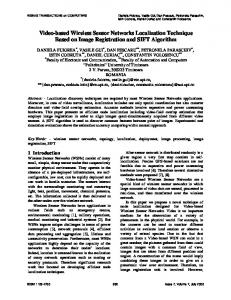
defined. These relationships are shown in the lower part of Fig. 1.
The problem of localization on sensor network can be thought as an optimization problem which is to find the most suitable positions of the sensors to fit the known inter-sensor distance measurements. Ravi Garg, et al [7] set the target function as the distance error between the known distances and the estimated
92
D is symmetric. The element d k ,l represents the distance between node k and node l. d k ,l is zero when
k =l . The target is to find the positions ( x1 , y1 ) , ( x2 , y2 ) , ( x3 , y3 ) , …, ( xn , yn ) . Note that the results obtained are of relative coordinates. We define the target function as (4). The relationship between ( xk , yk ) k = 1, 2,3,..., n and d k ,l 1 ≤ k < l ≤ n is expressed by x = diag (w × DT )
Fig. 1 The weights defined to connect the unknown coordinates with the known distances in n nodes situation
y = diag ( v × D ) where ⎡ x1 ⎤ ⎡ y1 ⎤ ⎢x ⎥ ⎢y ⎥ x = ⎢ 2⎥ , y = ⎢ 2⎥; ⎢�⎥ ⎢�⎥ ⎢ ⎥ ⎢ ⎥ x ⎣ n⎦ ⎣ yn ⎦ diag ( A) returns the main diagonal of A ; T
When the locations of the unknown nodes have been estimated, the following equation would calculate the distance between each pair of nodes (e.g. node k and l):
d k*,l = ( xk − xl ) 2 + ( yk − yl ) 2
(3)
The target function is the sum of the squared errors between the given distance measurements ( d k ,l ) and
n
2
(7)
DT is the transpose of D. It equals to D because D is symmetric. ⎡ 0 w1,2 � w1, n ⎤ ⎢w 0 � w2, n ⎥⎥ 2,1 w�⎢ ⎢ � � � � ⎥ ⎢ ⎥ ⎣⎢ wn ,1 wn ,2 � 0 ⎦⎥ is the matrix containing all weights between x coordinate and the distances. For example, wk ,l is the
the distance calculated based on the estimated location of the nodes ( d k*,l ).
E = 0.5 × ∑ ( d k ,l − d k*,l )
(6)
(4)
k , l =1 k l .
� v1, n ⎤ � v2, n ⎥⎥ � � ⎥ ⎥ � 0 ⎦⎥ is the matrix containing all weights between y coordinate and the distances. Because of the definition of d k*,l in (3) d k*,l is only ⎡ 0 ⎢v 2,1 v�⎢ ⎢ � ⎢ ⎣⎢ vn ,1
end of the iteration, the estimated positions of the sensors can be calculated by equations like equation (1) and (2). The detail of the algorithm is given below: 1. There are n nodes with unknown locations, ( x1 , y1 ) , ( x2 , y2 ) , ( x3 , y3 ) , …, ( xn , yn ) . The known information is the distances 2. between any pair of nodes. The distances can be written in a distance matrix with definition of: ⎛ d1,1 d1,2 � d1, n ⎞ ⎜ ⎟ d 2,1 d 2,2 � d 2, n ⎟ (5) D�⎜ ⎜ � � � ⎟ ⎜⎜ ⎟⎟ ⎝ d n ,1 d 2, n � d n , n ⎠
v1,2 0 � vn ,2
connected to xk , yk , xl , yl . Measurement d k ,l is related to xk , yk , xl , yl by weights in (6) (7). E in (4) is decreased for each iteration by updating w , v towards the direction of its derivative. dE (8) w i +1 = w i − K dw i where
93
0 ⎡ ⎢ dE dw dE ⎢ 2,1 = � dw ⎢ ⎢ ⎣⎢ dE dwn ,1 K is step size.
dE dw1,2 0
� dE dwn ,2 v i +1 = v i − K
� dE dw1, n ⎤ � dE dw2, n ⎥⎥ ⎥ � � ⎥ 0 � ⎦⎥
dE dv i
Assume: 1. There are n unknown nodes. 2. The distances between any pair of nodes are collected in the distance matrix below. ⎛ d1,1 d1,2 � d1, n ⎞ ⎜ ⎟ d 2,1 d 2,2 � d 2, n ⎟ D�⎜ ⎜ � � � ⎟ ⎜⎜ ⎟⎟ ⎝ d n ,1 d 2, n � d n , n ⎠ which is same as the statement in GDA. The positions of n nodes ( x1 , y1 ) , ( x2 , y2 ) , ( x3 , y3 ) , …, ( xn , yn ) are also the target that we want to find. We also use gradient descent to minimize the target function, which is defined as below
(9)
where
dE dv1,2 � dE dv1, n ⎤ ⎡ 0 ⎢ dE dv 0 � dE dv2, n ⎥⎥ dE ⎢ 2,1 = ⎥ � � � � dv ⎢ ⎢ ⎥ dE dv dE dv � 0 n ,1 n ,2 ⎣⎢ ⎦⎥ The steps of the methods are: ⎛ x1 y1 ⎞ ⎜ ⎟ x y2 ⎟ . 1. Initialize ⎜ 2 ⎜ � � ⎟ ⎜ ⎟ ⎝ xn yn ⎠ dE dE and in (8) and (9), 2. Compute dwk ,l dvk ,l
n
E = 0.5 × ∑ ( d k ,l − d k*,l ) k ,l =1 k