Qualcomm, Inc. 5775 Morehouse Dr. San Diego, CA 92121. Zafer Sahinoglu. Mitsubishi Electric Research Laboratories. 201 Broadway. Cambridge, MA 02139.
MITSUBISHI ELECTRIC RESEARCH LABORATORIES http://www.merl.com
Localization via TDOA in a UWB Sensor Network Using Neural Networks
Salih Ergut, Ramesh Rao, Ozgur Dural, Zafer Sahinoglu
TR2008-024
June 2008
Abstract In an Ultra-wide band (UWB) sensor network signal reflections from objects can be used to accurately determine the location. UWB signals are preferred in these types of sensor networks since they provide a very good resolution due to their fine time granularity. We propose an artificial neural network based localization to detect single object in a sensor network and compare its performance to Cramer-Rao bound and least squares estimator. Then we propose a two phase algorithm for multiple object detection and evaluate the algorithm for the case when there are two objects in a sensor network with three nodes. ICC 2008 (May)
This work may not be copied or reproduced in whole or in part for any commercial purpose. Permission to copy in whole or in part without payment of fee is granted for nonprofit educational and research purposes provided that all such whole or partial copies include the following: a notice that such copying is by permission of Mitsubishi Electric Research Laboratories, Inc.; an acknowledgment of the authors and individual contributions to the work; and all applicable portions of the copyright notice. Copying, reproduction, or republishing for any other purpose shall require a license with payment of fee to Mitsubishi Electric Research Laboratories, Inc. All rights reserved. c Mitsubishi Electric Research Laboratories, Inc., 2008 Copyright 201 Broadway, Cambridge, Massachusetts 02139
MERLCoverPageSide2
Localization via TDOA in a UWB sensor network using Neural Networks ¨ and Ramesh R. Rao Salih ERGUT ECE Department, University of California San Diego 9500 Gilman Dr. La Jolla, CA 92037
Ozgur Dural Qualcomm, Inc. 5775 Morehouse Dr. San Diego, CA 92121
Abstract—In an Ultra-wide band (UWB) sensor network signal reflections from objects can be used to accurately determine the location. UWB signals are preferred in these types of sensor networks since they provide a very good resolution due to their fine time granularity. We propose an artificial neural network based localization algorithm to detect single object in a sensor network and compare its performance to Cramer-Rao bound and least squares estimator. Then we propose a two phase algorithm for multiple object detection and evaluate the algorithm for the case when there are two objects in a sensor network with three nodes.
I. I NTRODUCTION Localization and tracking have been the focus of both the industry applications and academic research. There are two main approaches: active (e.g. [6], [7], [8], [9]) and passive ranging (e.g. [1], [2], [3], [4], [5]). In the active approach, tags are attached to objects to be tracked. These tags communicate with the nodes in the sensor network. Sensor nodes thus estimate the distances between the objects and the nodes which are used to locate the objects via triangularization. In the passive approach, objects do not wear tags and hence they are not collaborating with the positioning process. When the nodes communicate with each other, the presence of the object causes disturbances in the received signals. By analyzing these disturbances the location of the object can be estimated. Active tags are used in a new range of applications, including logistics (package tracking), security applications (localizing authorized persons in high-security areas), medical applications (monitoring of patients), family communications/ supervision of children, search and rescue (communications with fire fighters, or avalanche/earthquake victims), control of home appliances, and military applications [7] The systems built based on passive approach, on the other hand, have great potential for perimeter security and intrusion detection and they can be deployed around buildings or at the borders between countries. In this paper, we are considering the passive approach and proposing a neural network based algorithm to locate objects in an UWB sensor network. UWB is preferred in passive approach applications since it provides high resolution in time domain. UWB signals are
Zafer Sahinoglu Mitsubishi Electric Research Laboratories 201 Broadway Cambridge, MA 02139
perfect fit for wireless position location since they are able to resolve multipath components which provide accurate location estimates without the need for complex estimation algorithms. UWB sensor network provides a structure where low to medium rate communication and position location can be performed simultaneously. UWB technology not only facilitate centimeter accuracy in ranging but also make low power and low cost implementation of communication systems possible [7]. IEEE introduced a new standardization group 802.15.4a for low data rate communications combined with positioning capabilities which employs UWB technology as its physical layer. Our contributions in this study are: We first define a framework for passive localization in 802.15.4a sensor networks. Then we introduce a neural network based algorithm (NNBA) to locate a single object with the known sensor node positions. The main obstacle in locating multiple objects is to identify multipaths between different sensor nodes that correspond to different objects. We devise a two-step algorithm which uses NNBAs as building blocks to overcome this problem. Finally, we present performance results for locating two objects in a 3-node sensor network using this algorithm. We only consider the cases where the objects are relatively closer to the nodes, which enables us to work in a high SNR regime. Although we focus on two-dimensional sensor network, it is straightforward to extend the algorithms to threedimensional space. II. A
FRAMEWORK FOR DETECTING PASSIVE TARGETS
The IEEE 802.15.4a packet consists of a synchronization header (SHR) preamble, a physical layer header (PHR) and a data field. The SHR preamble is composed of the ranging preamble and the start of frame delimiter (SFD). The ranging preamble can consist of {16,64,1024,4096} symbols. The longer lengths {1024, 4096} are preferred for non-coherent receivers to help them improve the signal to noise ratio (SNR) via processing gain. Hence, they can have a better time-of-arrival estimate. The underlying symbol of the ranging preamble uses one of the length-31 ternary sequences, Si , in Table I. Each Si of length L = 31 contains 15 zeros and 16 non-zero codes, and has the much desired property of
Preambl
SFD
PHR
Payload
perfect periodic autocorrelation. In other words, the side-lobes at the periodic correlation output become zero; and what is observed at the receiver between two consecutive correlation peaks is only the power delay profile of the channel. Thus, the channel profile estimation does not get deteriorated by any side-lobe.
S2
TABLE I T HE BASIS PREAMBLE SYMBOL SET
S1
S1’s multipath profile at S2
Index S1 S2 S3 S4 S5 S6 S7 S8
a) B locates the target on an ellipse
S2
Symbol -1000010-1011101-10001-111100-110-100 0101-10101000-1110-11-1-1-10010011000 -11011000-11-11100110100-10000-1010-1 00001-100-100-1111101-1100010-10110-1 -101-100111-11000-1101110-1010000-00 1100100-1-1-11-1011-10001010-11010000 100001-101010010001011-1-1-10-1100-11 0100-10-10110000-1-1100-11011-1110100
Assume that ω is the transmitted UWB pulse waveform with unit energy, Tsym denotes the symbol duration, Nsym is the number of symbol repetition within the preamble, Tpri is the pulse repetition interval, Ns is the total number of pulses per symbol and Es denotes the symbol energy. Then, using any basis symbol Si , the preamble symbol waveform wi (t) and the preamble waveform Pi (t) can be written as r L−1 � Es X wi (t) = Si [j]ω t − jTpri (1) Ns j=0
S1
S1’s multipath profile at S2
b)
Fig. 1. Effects of external objects on the multipath profile of UWB signals. a) Multipath profile when there is not any object in the medium, b) Multipath profile is modified due to reflecting signals coming from the external object
Nsym −1
Pi (t) =
X
n=0
N[n]wi (t − nTsym
�
(2)
where N = [11...1]1×Nsym . A coherentNreceiver correlates the received waveform Yi (t) = Pi (t) h(t) with a template matched to wi (t). Then, assuming an AWGN channel the correlator output Ci (k) is ∞ Z (k+1)Ts X (Yi (t) + n(t))dt (3) Ci (k) =
1
k=0
Sensor
2
Target Sensor
3
Sensor1
0
1
Fig. 2. Using the multipath distance target object is located on an ellipse for each sensor pair. Target object is positioned at the intersection of all these ellipses.
kTs
where n(t) is the AWGN noise. Differences in Ci between two observations are indicative of changes in channel profile. As seen in Figure 1-a, the multipath profile is recorded when two sensor nodes are communicating with each other in the absence of any external object. When an object arrives, multipath profile alters due to receiving reflections from the object (see Figure 1-b). By estimating the time difference of arrival (TDOA), ∆t, between the direct path and reflecting path, the multipath distance, d, can be computed at the sensor node S2 as: d = |S1 − S2 | + c × ∆t where c is the speed of light and S1 and S2 are the locations of the sensors. Since d gives the sum of the distances from two sensor nodes whose locations are fixed, S2 can locate the object on an ellipse (Figure 1-b). We need at least three sensor pairs since the intersection of three or more ellipses uniquely identify the object location as it can be see in Figure 2.
j x1
1
6�� F
k1
x2
6�� F
6�� F
W
W
ij
jm Xn
jk
kp 6�� F
Output Vector
Input vector
j2
6�� F
Input Layer
Hidden Layer
Ouput Layer
Mean square error (MSE) is used to determine the compliance between the predicted output and computed network output. The exit criterion for the supervised learning is set on the value of MSE (e.g. when MSE is below 0.001). After successful termination of the learning process, the classification performance is determined by applying test data to the neural network. If the performance values meet the desired criteria at the end of the test, the structure of the neural network is completed and it is ready to classify any external data.
Output
V. S INGLE O BJECT D ETECTION Fig. 3.
Feed forward back propagation neural network architecture
Note that we do not need to transmit special signals between these sensor node pairs during the recording of the multipath profile, the preamble can simply be used for this purpose while these nodes are communicating with each other. This way there is no need for a secondary channel to transmit the recorded multipath profile to a data processing center, the same network can be used for this purpose. III. S IMULATION S ETUP In all simulations 1 × 1 unit grid is considered. Sensors are placed on a circle uniformly. For the sake of simplicity the shape of the objects and sensors are ignored and modeled as a point on the grid. Location of the objects are randomly generated. In this study, we only consider high SNR regimes where estimation errors can be modeled as white Gaussian [1], [2]. White Gaussian assumption holds when the errors are assumed to be due to thermal noise only. However, in reality there are other sources of errors, such as clock drifting, processor latencies, and interferences which may violate the white Gaussian assumption. We ignore all those types of errors in this paper. IV. N EURAL N ETWORK M ODEL Neural networks (NN) are a non-algorithmic methods, which use parallel computing technique. They imitate functioning of the brain. Even though inter-neuron communication speed is quite slow for the brain, parallel processing allows it to analyze very complicated data in a short period of time. Neural networks learn directly from current examples rather than programming [10]. Feed forward neural networks with multiple hidden layers have been widely used and showed to operate successfully (see Figure 3). Multi Layer Perceptron (MLP) learning algorithm is used in the training of the network. MLP is a back propagation algorithm and it computes the error at the output of the network and sets weights of neurons iteratively. This operation is spread out on all layers and the error in the output is reduced. Deviations between the real and the predicted values are computed to evaluate the learning success of the network.
Using time difference of arrival (TDOA) between the direct path and a reflecting path, the distance traversed by the multipath can be estimated. The multipath distance and the locations of the 2 sensors constitute an ellipse. We need at least three sensor pairs to figure out the location of the target object at the intersection of these ellipses. Assume that there are N nodes and a single object in the sensor network, and let (xci , yci ) denote the mid point between the i-th sensor pair, then (y − yc1 )2 (x − xc1 )2 + =1 2 a1 b21 (x − xc2 )2 (y − yc2 )2 + =1 a22 b22 .. . (y − ycN )2 (x − xcN )2 + =1 a2N b2N where ai and bi are the major and minor axes of the ellipse. There are different techniques to solve this set of non-linear equations. Least squares estimator is one approach. In this paper we propose to use artificial neural networks. We assume that the locations of the sensors are known apriori. In the training phase, a set of random points on the grid are generated. Total distance from a transmitter sensor node to the target object and from the target object to a receiver node is computed as: p p di = (x − xi1 )2 + (y − yi1 )2 )+ (x − xi2 )2 + (y − yi2 )2 )+ǫi
where di is the multipath distance between the i-th pair, (x, y) is the location of the object, (xik , yik ), k = 1, 2, is the coordinate of the k-th sensor node in the i-th pair, and ǫi N (0, σ 2 ) is the white Gaussian error. The multipath distances computed as above are then fed into the NN. The locations of the objects, i.e. (x, y), are used as the output to be matched by the NN as it is trained. During the verification phase, another set of random points are used in a similar fashion to evaluate the performance of the network. A. Simulation Results Figure 4 shows the performance of the NN with increasing number of sensors when the error variance is fixed, namely
−4
x 10 1
Cramer−Rao Bound Least Squares Estimate NN
3 sensors 4 sensors 5 sensors 6 sensors
0.9
MSE
0.8
0.7
1
CDF
0.6
0.5
0.4
0
3
4
5
6
Number of sensors
0.3
0.2
Fig. 5.
Comparing NN with Cramer-Rao and least squares estimates
0.1
0
0
0.005
0.01
0.015
0.02
0.025
Error
Fig. 4.
CDF of error with increasing number of sensors
σ 2 = 0.01. The error between the actual location, (x, y) and the estimated location, (ˆ x, yˆ) of the object is defined as p ˆ)2 + (y − yˆ)2 ε = (x − x
Cumulative distribution function (CDF) shifts to the right, and hence mean squared error (MSE) gets smaller, as the number of sensors are increased. Note that the transmit power of each sensor is limited, which is regulated by Federal Communications Commission (FCC) in the US. However, the total power transmitted by the sensor network is not limited. Therefore, one can benefit using more sensors to increase the accuracy of the estimates. Also the more sensors are there in the network, the more robust the network will become by tolerating individual sensor failures. B. Evaluating the performance of NN algorithm In this section we will compare the performance of our NN based algorithm with Cramer-Rao bound and a least squares based algorithm introduced in [3], [1]. Cramer-Rao bound gives a lower bound on the standard deviation of the estimation error, which can be used as a benchmark. 1) Cramer-Rao Bound: In [3], Cramer-Rao bound on the position estimation from multipaths is shown to be σ2 N2 where V (x) and V (y) are the bounds on the estimations of x and y coordinates, respectively and N is the number of transceivers, which are capable of both transmitting and receiving. Then the total variance becomes: V (x) = V (y) ∼
V (x) + V (y) ∼
2σ 2 N2
2) Least squares estimator: In [3], a two-step least squares estimator is proposed. First, using the multipath distances, piece-wise distances between the sensors and the object are estimated via least squares technique. Then using these estimates, the target object is located via triangulation. They showed that the variance of this technique is: 28σ 2 3N 2 3) Comparison: Figure 5 compares the MSE of the NN estimator with the Cramer-Rao bound and the least squares estimator as described above when the number of sensor networks are 3,4,5, and 6. The NN performance is comparable with the least squares estimator. As more sensor nodes are used the performance approaches to the Cramer-Rao bound. 2 σLS =
VI. M ULTIPLE O BJECT D ETECTION Tracking multiple objects in a sensor network becomes difficult since for each sensor pair it is hard to distinguish which multipath distance belongs to which object. In order to locate objects, one of the multipath distances from each sensor pairs are grouped into a set. Let N denote the number of sensors in the network and L denote the number � � of objects N to be detected. Then each set will contain = N (N2−1) 2 N (N −1) elements and therefore there will be M = L 2 different combination of sets to choose from. Furthermore, these sets can be grouped such that all multipath distance measurements are used. Each such group uses a distinct measurement from each of the N (N2−1) sensor pairs and hence each group contains exactly L sets since there are L objects. Therefore there are L
N (N −1) 2
=L
N (N −1) −1 2
L such groups. Only one of these groups corresponds to the right group of sets. As it can be seen in Figure 6, the overall detection algorithm is composed of two steps. In the first step, a set of multipath
d11 d.21 .. dN 1 d12 d.22 .. dN 2
�
C1 NNBA Block
-
xˆ1 yˆ1 xˆ2 yˆ2
x˜1 y˜1 C2
NNBA Block
x˜2 y˜2
CM NNBA Block
Ci
(.)2
ˆ d N,aN
Estimate Multipath
xˆL yˆL
xi
NNBA yi
�
� Fig. 7.
NNBA Block
x˜M
Fig. 6.
Two phase detector
measurements are fed as the input and a possible target location is estimated with a cost associated with it. Apriori known sensor locations are internally used in the cost computation. In the second step, the cost metrics for each set in the group are added together to form the group metric and the group with the lowest cost is selected. The block used in the first step (see Figure 7) uses the NNBA that is trained for estimating the single object location given multipath distances from each sensor pairs as described in Section V. The estimation, P˜i = (˜ xi , y˜i ), in conjunction with the apriori known sensor locations are used to estimate the multipath distances: dˆk,αk = |Sk1 − P˜i | + |P˜i − Sk2 | where dˆk,αk is the estimated multipath distance and Skj is the location of the j-th sensor node, j = 1, 2, of the k-th sensor pair. Here αk ∈ (1, 2, ..., L) indicates one of the L multipath distance measurements for this sensor pair. Then, the difference between the estimated and measured multipath distances are squared and added to compute the cost metric, Ci . N � �2 X Ci = dk,αk − dˆk,αk k=1
Group metric is then computed by adding the cost of individual sets in that group L X
S1
d1,a 1 d2,a 2 . . . dN,a N
y˜M
GCj =
- f
P
.. .
.. . d1L d.2L .. dN L
(.)2 . . .
ˆ ˆ d 1,a1d2,a2 . . . SN
Decision Box
(.)2
f - f
Cgj,k , where j = 1, 2, . . . , LN −1
k=1
where gi,k is the k-th cost index that belongs to the group i.
A. An example: Detecting two objects In this section, as an example for multiple target detection, we will consider the case when there are two objects in a sensor network with three nodes, i.e. N = 3, L = 2. At the end of this section we will discuss the simulation results. All possible input combination sets are: S1 S2 S3 S4 S5 S6 S7 S8
= = = = = = = =
{d11 , d21 , d31 } {d11 , d21 , d32 } {d11 , d22 , d31 } {d11 , d22 , d32 } {d12 , d21 , d31 } {d12 , d21 , d32 } {d12 , d22 , d31 } {d12 , d22 , d32 }
where di,j is the j-th multipath distance measured by the i-th sensor pair. Then the groups with complimentary sets becomes: G1 = {S1 , S8 } G2 = {S2 , S7 } G3 = {S3 , S6 } G4 = {S4 , S5 } Finally, the group with the minimum cost is selected. The CDF of the error between each the actual and the estimated location of the objects is plotted in Figure 8. As it can be seen from CDF in the same figure 1 target detection slightly performs better than 2 detection system as expected. This is mainly due to false selection of the final group, i.e. the group with minimum cost differs from the actual one. In the simulations this error was around 3.9%. Note that even when the wrong group was chosen, the estimated locations are still close to the actual targets, therefore the estimation error is not adversely affected and hence is still comparable to single target case. VII. R ELATED W ORK [1], [2], [3] study the Cramer-Rao bounds of passive localizations in an UWB sensor network for the asymptotic case
1 1 object 2 objects 0.9
0.8
0.7
errors will reduce since the location estimates are smoothed. For instance, a Kalman-Bucy filter similar to the one proposed in [11] can be used to filter out high variations in successive estimations. We only considered the high SNR regime. We would like to create models for low SNR cases and evaluate the performance of our neural network based algorithms with this model.
CDF
0.6
R EFERENCES 0.5
0.4
0.3
0.2
0.1
0
0
0.005
0.01
0.015
0.02
0.025
Error
Fig. 8. Comparing the performance of single object vs. two objects. Wrong decision 3.52%
with increasing number of sensors. They consider the cases where both the locations of the sensor networks are known apriori and unknown. They propose a semi-linear algorithm that uses least squares estimator for single target detection and compared the performance of their algorithm to CramerRao bounds. For multiple target detection they propose a heuristic centralized algorithm since they claim exhaustive search requires (L!)N M −1 iterations, where L is the number of objects, N and M are the number of transmitters and receivers, respectively. However we show that there are only LN (N −1)/2 different combinations to choose from, which is much smaller than the above figure when M = N . No error performance for the multiple target detection algorithm is provided and therefore we could not compare our algorithm with this research. [4], [5] experimentally compare the performance of active and passive detection algorithms and discuss the pros and cons of both techniques. Pulse positions are estimated by means of a high-resolution maximum likelihood estimator. VIII. C ONCLUSION AND F UTURE W ORK We discussed a framework to detect external object in an UWB sensor network and showed that neural networks can be used to detect single objects in such a network. We compared the performance of our algorithm with Cramer-Rao bound and least squares estimator. Then we proposed a two step algorithm to detect multiple objects. We simulated the case for two objects in a 3-node sensor network and showed that the performance is as good as detecting a single object in the same network. In addition, we will consider mobility of the objects in our future work. Note that adding the mobility in the system models provides extra information and therefore estimation
[1] Chang, C. and Sahai, A., “Object tracking in a 2D UWB sensor network,” in Conference Record of the Thirty-Eighth Asilomar Conference on Signals, Systems and Computers, 2004. [2] Chang, C. and Sahai, A., “Cramer-Rao-Type Bounds for Localization,” in EURASIP Journal on Applied Signal Processing, vol 2006, pages 1-13, 2006. [3] Chang, “Localization and Object Tracking in an UWB Sensor Network,” Master Thesis [4] R. Zet´ık, J. Sachs, P.Peyerl “UWB Radar: Distance and Positioning Measurements,” International Conference on Electromagnetics in Advanced Applications, Torino, Italy, Sept 2003 [5] R. Zetik, J. Sachs, R. Thoma “UWB Localization - Active and Passive Approach,” Implementation and Measurement Technology Conference (IMTC), Italy, May 2004. [6] A. Catovic, Z. Sahinoglu, “The Cramer–Rao Bounds of Hybrid TOA/RSS and TDOA/RSS Location Estimation Schemes,” IEEE COMMUNICATIONS LETTERS, VOL. 8, NO. 10, Oct 2004 [7] S. Gezici, Z. Tian, G. B. Giannakis, H. Kobayashi, A. F. Molisch, H. V. Poor, and Z. Sahinoglu, “Localization via Ultra-Wideband Radios,” IEEE Signal Processing Magazine, July 2005 [8] The Cricket Indoor Location System, http://cricket.csail.mit.edu [9] G. Opshaug, P. Enge, “GPS and UWB for Indoor Navigation,” GPS Conference, Salt Lake City, USA, Sep 2001 [10] N. Hardalac, N. Ercan, F. Hardalac, S. Ergut, “Classification of Educational Backgrounds of Students Using Musical Intelligence and Perception with the Help of Artificial Neural Networks,” Frontiers in Education Conference, 36th Annual, Oct. 2006 [11] S. Gezici, H. Kobayashi, H. V. Poor, “A New Approach to Mobile Position Tracking,” IEEE Sarnoff Symposium, Princeton, NJ, April 2004