Locally-connected Hierarchical Neural Networks for GPU-accelerated

Locally-connected Hierarchical Neural Networks for GPU-accelerated Object Recognition

Rafael Uetz and Sven Behnke Autonomous Intelligent Systems Group Institute of Computer Science VI University of Bonn, Germany [email protected], [email protected]

Abstract Convolutional neural networks have achieved good recognition results on image datasets while being computationally efficient, i.e., scaling well with the number of training patterns and the resolution of the patterns. Here we investigate a neural network model that has a similar hierarchical structure, but does not employ weight sharing. Instead, each neuron has a fixed receptive field with unique connection weights. To deal with the enormous number of weights resulting from this architecture, we implemented a parallel version of the model using Nvidia’s CUDA framework. This implementation is up to 82 times faster than a serial CPU implementation. Our model achieves state-of-the-art recognition performance on the NORB normalized-uniform dataset (2.87% error rate) and good results on the MNIST dataset (0.76% error rate). This suggests that large networks with local, non-shared connections might be an interesting architecture for object recognition tasks. To further evaluate the model, we created a large, publicly available training and testing set, which consists of objects extracted from the LabelMe natural image dataset.

1

Introduction

Recent theoretical and experimental results suggest that learning machines with deep, hierarchical structures may outperform flat architectures in solving difficult object recognition tasks [2, 5]. One such architecture is the Convolutional neural network (CNN) model [7], which has achieved stateof-the-art recognition results [4, 11] for the MNIST [8] and NORB [3, 9] datasets. In this paper, we propose a new neural network model called Locally-connected Neural Pyramid (LCNP). Its hierarchical structure is similar to models such as CNNs and the Neural Abstraction Pyramid [1]. However, the model does not employ weight sharing. Instead, each neuron has a fixed receptive field with unique connection weights, resulting in a much larger overall number of free parameters in the network compared to CNNs. This design decision is biologically motivated because the same connection structure is massively used by the human brain [6]. Despite the “curse of dimensionality”-hypothesis, our model achieves state-of-the-art results on the NORB dataset and good results on the MNIST dataset. To scale the model towards large object recognition tasks, we implemented it on GPU using the Nvidia CUDA framework [10]. The inherent parallelism of the local connectivity allows for high speedup factors compared to serial implementations. We do not describe the techniques used for the parallel implementation here because we focus on the network model and on the experimental results. 1

layer L-1

map of layer l+1

...

...

(a)

forward propagation

output layer

(b) map of layer l

layer 1

receptive fields

maps { layer 0

Figure 1: (a) Basic structure of the LCNP. (b) Receptive fields of two exemplary neurons.

2

The Locally-connected Neural Pyramid (LCNP)

The basic structure of our model is depicted in Figure 1 (a). There are L ≥ 1 regular layers and one output layer. Each regular layer l ∈ {0, . . . , L − 1} consists of at least one map, each map being a two-dimensional, square array of Nl × Nl neurons. The neuron model is the same as for multi-layer perceptrons [12]. We use the hyperbolic tangent as activation function. Maps of a specific layer all have the same size, whereas the size of maps in consecutive layers decreases by a factor of 2 so that Nl = 12 Nl−1 . The number of maps increases with each layer. This map structure ensures an increasing spacial invariance while the number of features for each position increases at the same time. In contrast to the regular layers, the output layer is a one-dimensional array of neurons, each representing one object class (one-hot encoding). Any two maps i and j of two consecutive regular layers l and l+1, l ∈ {0, 1, . . . , L−2}, respectively, can potentially be connected by a map connection. A map connection is a local connection structure between two maps where each neuron of map j has connections to an adjacent set of neurons in map i, called the receptive field of the neuron in map j. We chose the size of the receptive field to be 4 × 4 neurons. As the maps of layer l are twice as large as the maps of layer l + 1, the receptive fields overlap by 50 % in each dimension (see Figure 1 (b)). The highest regular layer L − 1 is fully connected to the output layer. The model is a pure feed-forward architecture. Learning is supervised and done via “plain-vanilla” backpropagation of error. We use a fixed learning rate ηl = 0.01·2L−l for map connections between layer l − 1 and l, l ∈ {1, . . . , L − 1}, and ηo = 0.0001 for the full connections between layer L − 1 and the output layer. All connection weights of the network are initialized randomly in the range [− √1n , √1n ], where n is the number of inbound connections for a specific neuron. Any map of each regular layer can be used as an input map by setting the activation values of its neurons to the desired input values. We apply two techniques to improve the recognition results: Firstly, several kinds of input maps are used. For the MNIST and NORB experiments described in Section 4, we used one input map resembling the raw grayscale images and four input maps resembling edge channels. The latter are calculated by four simple edge filters of different orientations, each with a 2×2 filter kernel. For the experiments with our LabelMe-12-50k dataset (described in the next section), we used three color channels instead of the grayscale channel, resulting in a total number of seven input maps. Secondly, the described input maps exist in every regular layer (not just in the lowest layer). This is done by first subsampling the original input image multiple times to the size of all regular layer’s maps. The described input channels are then calculated from these subsampled images. An advantage of this method is that the edge filters on lower layers extract fine-grained edges while those of higher layers extract coarse-grained edges. Similarly, the grayscale/color channels of lower layers represent fine details, whereas those of higher layers represent coarse regions.

3

The LabelMe-12-50k dataset

Our main goal in creating a new dataset was to use natural images with a great variety of object instances, lighting conditions, and angles of view. We chose to extract the training and testing images from the LabelMe dataset [13], which consists of more than 175,000 natural images, most of 2

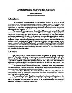
tree

car

building

window

person

keyboard

sign

clutter

Figure 2: Images from our training set. The object class is denoted below the image. them showing street and indoor scenes. We extracted 40,000 color JPEG images for training and 10,000 for testing. Each image is 256×256 pixels in size and either shows one centered object or a randomly selected region of a randomly selected LabelMe image (“clutter”). There are 12 object classes: “person”, “car”, “building”, “window”, “tree”, “sign”, “door”, “bookshelf”, “chair”, “table”, “keyboard”, and “head”. Further information on our dataset can be found on our website [14]. The dataset is also available for downloaded there. Figure 2 shows some images of the training set.

4

Experimental results

The recognition performance of our system was tested for three datasets: 1. The MNIST dataset [8], which consists of 70,000 grayscale images (60,000 for training and 10,000 for testing). Each image shows one handwritten digit. 2. The NORB normalized-uniform dataset [9], which consists of stereoscopic grayscale images of 50 toys, belonging to 5 categories. Each of the 48,600 images (24,300 for training and 24,300 for testing) shows one toy under different lighting conditions, elevations and azimuths. 3. The LabelMe-12-50k dataset described above. We used almost the same network structure and exactly the same parameters for training these datasets. The only difference was the number of input maps per layer: 5 for MNIST (grayscale + 4×edges), 7 for LabelMe-12-50k (3×color + 4×edges), and 10 for NORB (grayscale + 4×edges for each of the two stereoscopic channels). The network used for the measurements has five regular layers with the dimensions 256×256, 128×128, . . ., 16×16, so images of LabelMe-12-50k exactly fit into the maps of the lowest layer. Images of MNIST and NORB are initially enlarged to the same size, so the number of free parameters was equal for all datasets. In addition to the input maps, there are 2l non-input maps in each regular layer l ∈ {1, . . . , L − 1}, which have map connections to each map (input and non-input) of layer l − 1. Training images were randomly shifted by ±5 % of the map size during the training phase in order to improve generalization. Testing images were not shifted. The order of the training patterns was permuted randomly in each epoch. The recognition results are shown in Table 1. The training and testing error rates denote the percentage of incorrectly classified patterns of the whole training and testing set, respectively. All results were measured after training for 1000 epochs and are averaged over 10 epochs. However, similar recognition rates appeared much earlier. The testing error rate of MNIST was 3.86 % after one epoch and < 1 % after about 35 epochs. For NORB, it was 18.35 % after one epoch and < 5 % after about 20 epochs. We did not observe any significant overtraining (however, overtraining was a problem when not shifting the training images randomly). For our speed measurements, we used an Intel Core i7 940 CPU and an Nvidia GeForce GTX 285 graphics card on a Linux system with 12 GB of RAM. With the network structure described above, we obtained a speedup factor of 43.5 compared to a serial CPU version of the system (using one CPU core only), which was compiled with g++ and the O2 flag set. As we did not optimize the speed of the CPU version manually, the comparison of the speed serves as a rough baseline only. Depending on the specific network structure, the speedup factor is between 7.7 and 82.2 for very small and very large networks, respectively. The absolute GPU runtime for one training epoch of the LabelMe-12-50k dataset is 70.2 seconds when using the network structure described above. As one epoch consists of 40,000 images, the network processes about 570 images per second in the training phase. In the recall phase, the network processes about 1,356 images per second. 3

Dataset MNIST NORB normalized-uniform LabelMe-12-50k

Training error rate 0.03 % 0.05 % 3.77 %

Testing error rate 0.76 % 2.87 % 16.27 %

Table 1: Training and testing error rates

5

Conclusions

We presented a neural network model called Locally-connected Neural Pyramid (LCNP). The main concepts of this model are its hierarchical structure, the local connectivity without weight sharing, the use of subsampled inputs in all hierarchical layers, and the local preprocessing of the input patterns. The recognition performance of our model is competitive with state-of-the-art approaches. For the MNIST dataset, most approaches achieving better results (see [8] for a comprehensive list) use sophisticated preprocessing algorithms and/or unsupervised pretraining. For the NORB dataset, our results are (to our knowledge) the best ones achieved so far. The parallel implementation of our model allows for large-scale object recognition systems and an unprecedented size of training and testing datasets. Future work will focus on training with extremely large natural image datasets by keeping compressed JPEG images in the main memory and uncompressing them “on the fly” during the training phase. We are also planning to employ de-noising autoencoders for unsupervised pretraining and recurrent network structures for an iterative refinement of the output.

References [1] Sven Behnke. Hierarchical Neural Networks for Image Interpretation, volume 2766 of Lecture Notes in Computer Science. Springer, 2003. [2] Yoshua Bengio. Learning deep architectures for AI. Foundations and Trends in Machine Learning 2:1, 2009. [3] Fu Jie Huang and Yann LeCun. The Small NORB Dataset, V1.0, 2005. http://www.cs.nyu.edu/ ˜ylclab/data/norb-v1.0-small/. [4] Fu-Jie Huang and Yann LeCun. Large-Scale Learning with SVM and Convolutional Nets for Generic Object Categorization. In Proc. CVPR’06. IEEE Press, 2006. [5] Kevin Jarrett, Koray Kavukcuoglu, Marc’Aurelio Ranzato, and Yann LeCun. What is the best multi-stage architecture for object recognition? In Proc. International Conference on Computer Vision (ICCV’09). IEEE, 2009. [6] Eric R. Kandel, James H. Schwartz, and Thomas M. Jessel. Principles of Neural Science. McGraw-Hill, 4 edition, 2000. [7] Yann LeCun, Leon Bottou, Yoshua Bengio, and Patrick Haffner. Gradient-based learning applied to document recognition. Proceedings of the IEEE, 86(11):2278–2324, 1998. [8] Yann LeCun and Corinna Cortes. The MNIST database of handwritten digits. http://yann.lecun. com/exdb/mnist/. [9] Yann LeCun, Fu Jie Huang, and Lon Bottou. Learning methods for generic object recognition with invariance to pose and lighting. In Proceedings of CVPR04. IEEE Press, 2004. [10] NVIDIA Corporation. CUDA Programming Guide, version 2.2, 2009. [11] Marc’Aurelio Ranzato, Christopher Poultney, Sumit Chopra, and Yann LeCun. Efficient learning of sparse representations with an energy-based model. Advances in Neural Information Processing Systems, 19, 2006. [12] Frank Rosenblatt. The perceptron: A probabilistic model for information storage and organization in the brain. Psychological Review, 65(6), 1958. [13] B. C. Russell, A. Torralba, K.P. Murphy, and W. T. Freeman. LabelMe: a database and web-based tool for image annotation. International Journal of Computer Vision, 77(1–3):157–173, 2008. [14] Rafael Uetz. The LabelMe-12-50k dataset. datasets.html.

http://www.ais.uni-bonn.de/download/

4