ProbLog Technology for Inference in a Probabilistic First Order Logic Maurice Bruynooghe and Theofrastos Mantadelis and Angelika Kimmig and Bernd Gutmann and Joost Vennekens and Gerda Janssens and Luc De Raedt1 Abstract. We introduce First Order ProbLog, an extension of first order logic with soft constraints where formulas are guarded by probabilistic facts. The paper defines a semantics for FOProbLog, develops a translation into ProbLog, a system that allows a user to compute the probability of a query in a similar setting restricted to Horn clauses, and reports on initial experience with inference.
1
Introduction
A problem for languages that combine probability theory with expressive logical formulas is that probabilistic and logical knowledge might interact in complex ways, leading to a semantics that is too complicated to understand, and inference/learning that is too slow to be of practical use. Initial research into Probabilistic Logic Learning therefore mainly focused on adding probabilities to restricted logical languages, such as definite clause logic [3, 13]. Since then, the trend has been to extend the expressivity of the logical language, e.g., to normal clauses [10]. In the past few years there has been a lot of attention to Markov Logic [12], a probabilistic logic used in statistical relational learning [1]. Markov Logic consists of a set of weighted logical formulas each of which can be regarded as a soft constraint. If such a soft constraint is violated by a possible world, the probability of the world does not become zero, as in first order logic, but gracefully decreases. The higher the weight, the harder the constraint becomes, with infinite weights corresponding to the usual logical interpretation. While Markov Logic has been very successful as a framework for statistical relational learning and has been applied in several challenging applications, such as natural language processing and entity resolution, Markov Logic models are hard to interpret and not really suitable as a knowledge representation tool. The reason is that the weights cannot directly be interpreted as probabilities and also that the probability of a formula depends non-linearly on all weights in the theory. This paper contributes a new formalism, called First Order ProbLog, using the Markov Logic idea of soft constraints, but in which each first order formula is annotated with the probability that a grounding of the formula – independently of anything else – holds. This gives a logic very similar to that of Nilson [9]. The questions arise whether inference is feasible and how one can cope with inconsistency. These questions are explored in this paper. Using ideas of Stickel [15], we translate a theory in our logic into a ProbLog program [5] that also includes clauses for inferring inconsistency (with head false). We show how to use the ProbLog machinery to assign a minimal and a maximal probability to the truth of the query while taking consistency requirements into account. 1
Katholieke Universiteit Leuven, email:
[email protected]
2
First Order ProbLog and its Semantics
A ProbLog program [4, 5] consists of a set of facts annotated with probabilities – called probabilistic facts – together with standard definite clauses that can have positive and negative probabilistic facts in their body. The semantics is defined through belief sets which correspond to least Herbrand models of the clauses together with subsets of the probabilistic facts. If fact fi is annotated with pi , fi is included in a belief set with probability pi and left out with probability 1 − pi . The different facts are assumed to be probabilistically independent, however, negative probabilistic facts in clause bodies allow the user to enforce a choice between two clauses. In this paper we define FOProbLog, a language similar to ProbLog, but using full first order logic formulas instead of definite clauses. A FOProbLog statement is of the form ∀x.Ψ1 : α1 ∨ . . . ∨ Ψn : αn where the αi are non-zero probabilities with sum 1 and the Ψi are first order formulas with free variables included in x. If Ψi is true, it can be omitted (in which case the sum of the probabilities becomes smaller than 1); if α1 = 1, it can be omitted as well. These formulas express independent beliefs about the world. Each belief is disjunctive: we believe that for each grounding of x exactly one of a number of possibilities holds, but we don’t know which one, so we attach a probability to each of the disjuncts. We can now have a number of different ”complete belief sets”, which are formed by believing precisely one disjunct from every grounded disjunction according to its probability. Ex. 1 Our running example uses a domain with a single constant F loris and theories consisting of subsets of the following formulas (1) (2) (3) (4)
male(F loris) : 0.4 ∨ f emale(F loris) : 0.6 ∀x.(cs(x) → male(x) : 0.8) ∨ (cs(x) → f emale(x) : 0.2) ∀x.¬(male(x) ∧ f emale(x)) cs(F loris)
If the theory contains only formula (1), expressing a prior belief about the name Floris being male or female, each complete belief set either includes the fact male(F loris) (with probability 0.4) or the fact f emale(F loris) (with probability 0.6). After adding the second formula, each complete belief set also contains one of cs(F loris) → male(F loris) and cs(F loris) → f emale(F loris). One of the resulting four belief sets, with probability 0.8 · 0.6, contains the formulas f emale(F loris) and cs(F loris) → male(F loris). Adding the third formula to the theory, the extension of the latter belief set allows one to infer ¬male(F loris) and ¬cs(F loris). Belief sets in FOProbLog can be inconsistent. One should assign zero probability to such belief sets. With s a total choice and c(s) ex-
pressing consistency of s, P (s|c(s)), the normalized probability of a total choice s, is given by P (s)·P (c(s)|s)/P (c(s)) where P (c(s)|s) is either 1 or 0. Ex. 2 Using all four formulas of Example 1 makes the belief set with formulas f emale(F loris), cs(F loris) and cs(F loris) → male(F loris) (as well as another one) inconsistent. The probability of an inconsistent belief set is 0.8 · 0.6 + 0.4 · 0.2 = 0.56. Normalizing the probabilities of the two consistent belief sets, we obtain 0.4·0.8/(1−0.56) = 0.73 for the one containing male(F loris) and 0.27 for the one with f emale(F loris). Using all our independent formulas about maleness, we thus derive that F loris is more likely male than female, contrary to the belief about the name F loris. While the above example can be modeled in ProbLog, the probabilities inferred there will have a different meaning, as ProbLog adopts a different view on consistency. In a ProbLog program containing clauses male(F loris). with probability 0.4 and male(X):-cs(X). with probability 0.8, those clauses together define the male predicate and, by closed world assumption, also ¬male, the equivalent of f emale. There are 4 different belief sets, one with both clauses, two with one clause and one without clauses, but none with an inconsistent belief set where F loris is both male and not male. The probability of male(F loris) is thus 0.8 + 0.4 − 0.8 · 0.4 = 0.88 instead of 0.73. In the rest of the paper, we use a more basic form of FOProbLog which, similarly to ProbLog, distinguishes probabilistic facts from the logical part of a theory. Def. 1 (FOProbLog theory) A FOProbLog theory T = (P F, Φ) consists of a probabilistic part P F and a logical part Φ. Its predicates are split into sets ΣP and ΣL of probabilistic and logical predicates, respectively. P F contains probabilistic facts of the form pf (x) : α, with α a non-zero probability, x n different variables and pf /n ∈ ΣP . Each ground instance pf (x)θ of such a fact is true with probability α, and is not a grounding of any other probabilistic fact. Different instances (of the same or of different probabilistic facts) are probabilistically independent. An assignment of a truth value to a ground instance of a probabilistic fact is called atomic choice, an assignment to all of them a total choice. The probability prob(s) of a total choice s is the product of all αi for true instances pfi (x)θ : αi and all (1 − αj ) for false instances pfj (x)θ : αj . The logical part Φ of the theory consists of a set of implications ∀x.P (x) → F (x), where F (x) is a first-order formula with free variables x using only predicates from ΣL , and P (x) is a conjunction of literals with predicates from ΣP 2 . Ex. 3 Formulas (1)-(4) of Example 1 are now written as (1a) (1b) (1c) (2a) (2b) (2c) (3) (4)
pf mn(F loris) : 0.4 pf mn(F loris) → male(F loris) ¬pf mn(F loris) → f emale(F loris) pf cs(x) : 0.8 ∀x.pf cs(x) → (cs(x) → male(x)) ∀x.¬pf cs(x) → (cs(x) → f emale(x)) ∀x.¬(male(x) ∧ f emale(x)) cs(F loris)
The probabilistic part of formulas (3) and (4) is true and omitted. 2
A formula ∀x.Ψ1 : α1 ∨ . . . ∨ Ψn : αn is split into n formulas ∀x. Pi (x) → Ψi (x) and n − 1 probabilistic facts are introduced, their probabilities are computed and the probabilistic part Pi (x) of each formula contains a conjunction of probabilistic literals as described in [4].
To define the semantics of our logic, we fix a domain D and consider the set WD of all possible worlds in D, i.e., each I in WD is an interpretation for the vocabulary of the theory with D as its domain; in particular I assigns true or false to each probabilistic and each logical ground atom. Notation 1 In what follows, we use I |= s with I an interpretation and s a total choice to express that I makes the same truth assignments to the probabilistic facts as s. We often say I extends s. Def. 2 (Semantics) Let T = (P F, Φ) be a theory and D a domain. Let Cons be the set of total choices s such that there exists an interpretation I that extends s (I |= s) and is a model of Φ (I |= Φ), i.e., the total belief set corresponding to the total choice is consistent. d prob(s) (the normalized probability P of a total choice) is given by prob(s) · prob(s ∈ Cons|s)/ s∈Cons prob(s) where prob(s ∈ Cons|s) is 1 when s is consistent and 0 otherwise. A probability distribution µ over WD is a model of T , denoted µ |= T , if and only if (i) for all I : I 6|= Φ implies µ(I) = 0; (ii) for P d each total choice s: prob(s) = I|=s µ(I). The theory is inconsistent when no consistent total choice exists. In that case, no probability distribution is defined. Note that the normalization introduced here corresponds to conditioning on total choices with consistent extensions, which will be exploited in Section 3 to calculate probabilities of queries. In contrast to the above informal exposition, where belief sets contained logical formulas and hence had interpretations over the logical predicates only, now interpretations assign truth to both probabilistic and logical predicates. Ex. 4 In our example, with two probabilistic and three logical predicates and a single constant, we now have 32 possible interpretations. However, as before, only two of the four total choices can be extended in a belief set that is a model of the logical part; moreover, these models are unique. One of them is the belief set {pf cs(F loris), pf mn(F loris), cs(F loris), male(F loris)}. It extends the total choice {pf cs(F loris), pf mn(F loris)}, is a model of the logical part of the theory and is assigned probability 0.73 in the probability distribution that is a model. The other one, {cs(F loris), f emale(F loris)}, extends the total choice where both probabilistic atoms are false; it is assigned probability 0.27. The total choices that make one probabilistic atom true and the other one false cannot be extended in a model of the logical part; their probability mass has been redistributed over the other ones. In the above example, there is at most one belief set that extends a total choice and hence only one probability distribution that is a model. This does not hold in general. FOProbLog theories impose constraints, and any distribution satisfying these constraints is a model. Instead of making additional assumptions (such as the principle of indifference) to choose a specific distribution, we will restrict ourselves to sound inference, and will infer probability intervals only. Ex. 5 Consider a theory consisting of the probabilistic fact pf (x) : 0.7 and the logical formula ∀x.pf (x) → p(x) with a single element domain {A}. The total choice pf (A) can be extended into the belief set {pf (A), p(A)} and hence µ({pf (A), p(A)}) = 0.7. The empty total choice can be extended in two ways, namely ∅ and {p(A)}; hence µ(∅) + µ({p(A)}) = 0.3. Any distribution that satisfies the latter constraint is a model. The principle of indifference would assign probability 0.15 to each of the latter two belief sets and hence 0.85 to p(A) and 0.15 to ¬p(A). We infer that the probability of p(A) is in the interval [0.7, 1.0] and that of ¬p(A) in [0.0, 0.3].
3
Inference
We are now interested in deciding what the theory T allows us to conclude over the probability of some query formula Q. ˆ of modFor each given domain, T has a non-empty set M ˆ els µ. Each µ ∈ M assigns a particular probability µ(Q) = P I|=Q µ(I) to Q, yielding, in general, a non-empty probability interval [minµ∈M ˆ µ(Q), maxµ∈M ˆ µ(Q)]. We are now interested in the inference task of determining this interval. Because maxµ∈M ˆ µ(Q) must be equal to 1 − minµ∈M ˆ µ(¬Q), we can restrict attention to the computation of a lower bound on the probability of a query. As the following theorem shows, we can compute this lower bound without having to consider any specific model µ of T . ˆ be the non-empty set of models of a consistent Theorem 1 Let M P d theory T . Then minµ∈M ˆ µ(Q) = s|=Q prob(s), where s |= Q means that Q holds in all I ∈ WD such that I |= s. Proof 1 Let WQ = {I|I |= Q}Pand WSQ = {I|∃s : I |= s ∧ s |= Q}. By definition, µ(Q) = I∈WQ µ(I). Also by definition, P P P d prob(s) = I∈WSQ µ(I). Obviously, I∈WQ µ(I) ≥ Ps|=Q µ(I). To prove the theorem, it suffices to show that there I∈WSQ 0 exists a probability distribution µ that is a model and for which the equality holds. The equality holds if µ0 assigns 0 probability to all I ∈ WQ \ WSQ . For such I, we can distinguish two cases. Either I restricted to the probabilistic atoms gives a total choice that cannot be extended into a consistent belief set, in which case all distributions that are a model assign 0 probability to I. Or I restricted to the probabilistic atoms gives a total choice s with at least one I 0 extending s such that I 0 6|= Q. In this case, µ0 can be chosen to assign all the d probability mass prob(s) to interpretations that are not models of Q 0 and hence set µ (I) = 0. Hence µ0 (I) = 0 for all I ∈ WQ \ WSQ . The normalized probability of a total choice that can be extended into a consistent belief set is obtained by dividing its probability by the probability of all such total choices. The latter is the complement of the probability of those total choices where this is not possible, that is, the belief sets containing f alse. d Furthermore, recall that prob(s) = 0 for total choices without consistent extension. Hence, we also have minµ∈M ˆ µ(Q) = “P ” ” “ P s|=Q∧¬false prob(s) / 1 − s|=false prob(s) , which in fact
that describes how to use Prolog technology for building a first order logic theorem prover comes to the rescue and allows us to convert FOProbLog theories into ProbLog programs. The basic idea of Stickel’s work is to transform formulas into clausal form and to encode each n-literal clause l1 ∨ . . . ∨ ln by n Horn clauses of the form li :-not(l1 ), . . . , not(li−1 ), not(li+1 ), . . . , not(ln ).. To obtain Horn clauses, negative literals are encoded by positive ones: For each predicate p/n, Stickel introduces a not p/n and the negation of p(t) is replaced by not p(t). In the context of FOProbLog, for each formula ∀x.P (x) → F (x), the logical part F (x) is converted in clausal form, Stickel’s transformation is applied to the resulting clauses, and the conjunction P (x) is added to the bodies of the final Horn clauses. Ex. 7 Applying the transformation to our example gives the following ProbLog program (we switch to Prolog notation for constants and variables): (1a) (1b) (1c) (2a) (2b) (2b) (2c) (2c) (3a) (3b) (4)
0.4::pf_mn(floris) male(floris) :- pf_mn(floris). female(floris) :- not(pf_mn(floris)). 0.8::pf_cs(X) male(X) :- cs(X), pf_cs(X). not_cs(X) :- not_male(X), pf_cs(X). female(X) :- cs(X), not(pf_cs(X)). not_cs(X) :- not_female(X), not(pf_cs(X)). not_female(X) :- male(X). not_male(X) :- female(X). cs(floris).
The transformation also has to generate clauses with f alse in the head, as those are needed during inference to take consistency into account. One way to do so is to use the knowledge that a resolution proof must use at least one clause pf (x) → not(l1 ) ∨ . . . ∨ not(ln ) with only negative literals (to have all such clauses as ”set of support”). By adding false:-l1 , . . . ln , pf (x) for each such clause, we ensure that all proofs of false employ such clauses. Alternatively, one can use the positive clauses (clauses with only positive literals) as set of support. Simply adding a clause false:-p(X), not p(X) for each logical predicate p/n is also possible, but will typically result in a lot of redundant proofs. Ex. 8 In our example, using negative clauses as set of support would add: false :- male(X), female(X).
whereas using positive clauses would add:
corresponds to the conditional probability prob(Q|¬false). Ex. 6 Let us reconsider the theory consisting of pf (x) : 0.7 and ∀x.pf (x) → p(x). The query p(A) can be proven with a total choice that includes the probabilistic fact pf (A). As no total choice results in inconsistency, this gives a minimal probability of 0.7. No proofs are possible for ¬p(A), hence the maximal probability of p(A) is 1. The number of total choices is exponential in the number of probabilistic facts, hence it is not feasible to evaluate a query for each total choice. More promising is the ProbLog approach that enumerates all proofs in terms of the probabilistic facts they use and encodes this information in a Binary Decision Diagram (BDD), which can be used to compute the probability of the query [5]. The main difference is that we do not work with Horn clauses but with full first order logic, hence we cannot, as in ProbLog, use the SLD proof procedure to enumerate proofs. However, for quickly building a first prototype and for making maximal use of the ProbLog technology, it is interesting to stay as much as possible within Prolog. Here the work of Stickel [15]
false :- not_cs(floris). false :- not_male(floris), pf_mn(floris). false :- not_female(floris), not(pf_mn(floris)).
Stickel additionally needs to modify certain parts of the inference mechanism. First, Prolog’s input resolution is extended with ancestor resolution: resolution between the current goal and one of the ancestors in the linear chain from query to current goal. A convenient way to do so in the setting of Prolog’s depth first left to right execution policy is to keep track of the selected literals with uncompleted proof. If in the uncompleted proof of a literal p(t) (or not p(t)), its negation not p(s) (or p(s)) is selected, the latter literal can be resolved by unifying its atom with the atom of the former (i.e. unifying t with s) [15]. Also, care is required to avoid unsound unification. In general, some unifications may have to be replaced by a sound variant that performs an occur check. When proving queries in knowledge bases, it is unlikely that the occur check is needed. Finally, performing iterative deepening avoids that the search gets trapped in an infinite branch.
¬sameBib(b1, b2) ¬sameAuthor(a1, a2) ∀ b1, b2, b3 : sameBib(b1, b2) ∧ sameBib(b2, b3) → sameBib(b1, b3) ∀ b1, b2, a1, a2 : author(b1, a1) ∧ author(b2, a2) ∧ sameAuthor(a1, a2) → sameBib(b1, b2)
not_author(B,A) :- not(author(B,A)). not_hasWordAuthor(A,W) :not(hasWordAuthor(A,W)). false :- author(B,A), not_author(B,A). false :- hasWordAuthor(A,W), not_hasWordAuthor(A,W).
∀ a1, a2, w : hasW ordAuthor(a1, w) ∧ hasW ordAuthor(a2, w) → sameAuthor(a1, a2)
sameBib(B,B). sameAuthor(A,A). not_sameBib(B1,B2) :- B1 \= B2, pf1(B1,B2). not_sameAuthor(A1,A2) :- A1 \= A2, pf2(A1,A2).
∀a1, a2, w : ¬hasW ordAuthor(a1, w) ∧ hasW ordAuthor(a2, w) → ¬sameAuthor(a1, a2)
false :- domBib(B), not_sameBib(B,B). false :- domAuthor(A), not_sameAuthor(A,A).
Figure 1. A key part of the logical theory.
Given the transformed theory and a query Q, we can now use ProbLog’s machinery to construct two Boolean formulas ψ and φ representing the proofs of Q and the proofs of false, respectively. The formula ψ ∧¬φ thus restricts the proofs of Q to consistent belief sets, whereas φ is used for normalization, i.e. minµ∈M ˆ µ(Q) is obtained by P (ψ∧¬φ)/(1−P (φ)), where both intermediate results are calculated using ProbLog’s BDD algorithm. For the running example, we obtain φ = (¬pf cs(f loris)∧pf mn(f loris))∨(pf cs(f loris)∧ ¬pf mn(f loris)), and, for the query ? − male(f loris), ψ ∧ ¬φ = pf cs(f loris) ∧ pf mn(f loris).
4
A case study
To assess performance in practice, we explored an application of Markov Logic in entity resolution [14]. We will first review some details of the application, and then describe how to encode key parts of it directly in ProbLog. In this application, a fact database containing information about bibliographic entries such as authors and titles is combined with a probabilistic first order theory describing when two database references of the same type are likely the same. The purpose of entity resolution is to compute the probability that two keys or two authors (e.g. author_william_w_cohen_ and author_w_w_cohen_) refer to the same object, i.e., to be able to get probabilities for the queries sameBib(b1, b2) and sameAuthor(a1, a2), as well as for not sameBib(b1, b2) and not sameAuthor(a1, a2). Part of the facts database is a binary encoding of a ternary relation between authors, paper title and publication venue. A tuple (author, paper, venue) is encoded as author(bib, author), title(bib, paper) and venue(bib, venue) with bib an arbitrary key identifying a bibliographic entry. As formulas for authors, papers and venues are similar in structure, we will restrict our discussion to those concerning authors and bibliographic entries. Authors are strings (extracted from web pages) that are composed from different words (e.g. author_william_w_cohen_ and author_w_w_cohen_ are composed of the words word_cohen, word_w, and word_william. This information is encoded in the database relation hasW ordAuthor(author, word). Figure 1 shows the first order logic formulas used in [14] to model a key part of the application. A first simple set of rules states that different strings refer to different authors or different bibliographical
sameBib(B1,B3) :- sameBib(B1,B2), sameBib(B2,B3), pf5(B1,B2,B3). not_sameBib(B1,B2) :- sameBib(B2,B3), not_sameBib(B1,B3), pf5(B1,B2,B3). not_sameBib(B2,B3) :- sameBib(B1,B2), not_sameBib(B1,B3), pf5(B1,B2,B3). sameBib(B1,B2) :author(B1,A1), author(B2,A2), sameAuthor(A1,A2), pf9(B1,B2,A1,A2). not_sameAuthor(A1,A2) :author(B1,A1), author(B2,A2), not_sameBib(B1,B2), pf9(B1,B2,A1,A2). not_author(B1,A1) :sameAuthor(A1,A2), author(B2,A2), not_sameBib(B1,B2), pf9(B1,B2,A1,A2). not_author(B2,A2) :sameAuthor(A1,A2), author(B1,A1), not_sameBib(B1,B2), pf9(B1,B2,A1,A2).
Figure 2. Key clauses in ProbLog.
entries, respectively. The next formula is an example of rules expressing that the relations about sameness are likely transitive, while the remaining ones link authors to bibliographical entries and words to authors, respectively. Figure 2 shows the result of translating those formulas into ProbLog. We cannot blindly translate the first order theory. The main reason is that the closed world assumption is applied on the large database. Explicitly adding all negative facts would result in an exponential blow-up in the size of the logical theory. Therefore, we instead use negation as failure to encode them and add the first group of rules to our theory. Note that calls to these predicates are correctly executed only when all arguments are ground. This need not be a problem because ProbLog aims at inference of ground queries. Another difficulty – if we stick to the negative clauses as set of support – is that, for each tuple (b, a) not in the database, we would need to add a clause false :- author(b, a). As we cannot enumerate all such pairs (b, a), we resort to a different approach to define f alse. Using a positive set of support, we should add f alse :- not author(b, a) for each pair in the author relation. As the theory does not contain clauses with author/2 in the head, we can use the author relation to generate the pairs. Furthermore, this approach introduces less redundancy in the search space of proofs for f alse than the approach of simply adding a rule f alse :- p(X), not p(X) for each of the predicates author/2, hasW ordAuthor/2, sameAuthor/2, and sameBib/2. The next block of rules states that identical strings refer to identical entities (with certainty), different strings to different entities (with a rather high probability). As we have added positive clauses, we also have to add the next block of extra rules for proving
3500 3000
Proof Collection (ms) Proof Collection (ms)
false. Here domBib/1 and domAuthor/1 are used to generate the values for the keys and the authors respectively (appropriate ground facts have to be added to the database). Each clause about transitivity gives rise to three ProbLog clauses, which form the next block. Note that loop checking as well as ancestor resolution are important for doing exact inference with these clauses. The clauses linking authors to bibliographic entries give rise to the last block. Finally, as the rules linking authors and words can be translated in the same way as the previous clauses, we do not further elaborate them. However, one important observation is that the sharing of words in different author names, paper titles, and venues, results in a densely connected network to the point that almost for every pair (b1, b2) of keys, one can prove sameBib(b1, b2) as well as not sameBib(b1, b2). Hence, there are a lot of inconsistent total choices, it is essential to perform normalization and to execute the f alse query. Clearly, this is very demanding.
2500 2000 3500 1500 3000 1000 2500 500 2000 0 10
1500 Depth 1 1000
6
Discussion
In FOProbLog, probabilities are associated with formulas in first order logic. The assumption that these formulas are independent allows
40
50
60
70
80
90
100
Depth 2
Depth 3
Depth 4
Depth 5
Depth 6
Depth 7
500
Figure 3. Friends experiments. 10
Experiments
20
30
40
50
60
70
80
90
100
Domain Size Depth 1
Depth 2
Depth 3
Depth 4
Depth 5
Depth 6
Depth 7
2500000
2000000
Proof Collection (ms)
We set up experiments to investigate the feasibility of inference in FOProbLog. We focus on the query false, as this can involve all possible queries in a theory and thus is the most challenging query. We used a version of ProbLog with tabling [6] which we extended with ancestor resolution and iterative deepening as suggested by Stickel [15]. Experiments are performed on an Intel Core 2 Duo CPU at 3.00GHz with 2GB RAM running Ubuntu 8.04.2 Linux. In our experiments ProbLog is used to first collect the proofs and construct a Boolean formula for false and to then compute the probability by constructing a BDD. The first experiment uses the following FOProbLog theory ∀x, y, z. pf 1(x, y, z) → (F r(x, y) ∧ F r(y, z) → F r(x, z)) ∀x. pf 2(x) → (Sm(x) → Ca(x)) ∀x, y. pf 3(x, y) → (F r(x, y) → (Sm(x) ↔ Sm(y))) and randomly generated databases to investigate the influence of the domain size and the maximum depth used in iterative deepening. The latter limits transitive closure. The runtimes to obtain the Boolean formula representing false are presented in Figure 3; a missing bar indicates that the experiment failed to properly terminate. We notice that the search space grows exponentially with the depth limit, while the influence of the domain size is less drastic. Assessing the probability of the Boolean formula through BDDs is feasible within one minute for most of these experiments. The second experiment uses the entity resolution model of Section 4 with the full database of [14] containing 1295 bibliographic entries involving roughly 90 authors, 400 venues, 200 titles and 2700 words. Figure 4 shows the time to obtain the Boolean formula representing false for increasing maximum search depth. The results confirm that search time increases exponentially, as can be expected for such a densly connected problem. The limiting factor of our current prototype is the size of the resulting BDDs; in this application, they are too large to be constructed within a time limit of one hour. It is worth mentioning that in both experiments, the Boolean formulas for other queries are far smaller. However, in most cases, the time still increases exponentially with the depth bound. Furthermore, our current results do not permit general conclusions about the gap between minimal and maximal probabilities obtained for each query.
30
Domain Size
0
5
20
1500000
1000000
500000
0 1
2
3
4
5
Depth Bound Bibliography
Figure 4. Bibliography experiments.
us to define a semantics based on complete belief sets. Inference in FOProbLog is the task of calculating the probability that a query can be proven in a randomly selected complete belief set. Randomly selected belief sets can be inconsistent. The probability of such a selection can be computed. Normalization assigns 0 probability to inconsistent total choices and redistributes their probability mass over the consistent ones. The probability of the truth of a query is computed with respect to consistent total choices. One could argue that inconsistency is an indication of the violation of the independence assumption. Interestingly, inconsistent belief sets typically arise after adding factual knowledge (adding cs(Floris) or adding the database of bibliographical information). This factual knowledge can be seen as evidence that excludes certain belief sets. Inconsistency in the non-factual part is thus not an indication of poor design, as it can make sense to add a formula as evidence to an existing theory. This refines the theory by ruling out certain complete belief sets, and hence causes a redistribution of the probability mass. A related issue is the presence of redundant formulas. One might consider a situation where two independent experts contribute exactly the same formula to a theory, each of them claiming this formula with probability p1 and p2 respectively. The probability that
this formula then holds in a complete belief set is p1 + p2 − p1 · p2 . This makes sense when the expertise is really based on different knowledge. However, with each additional independent expert coming up with the same formula and assigning some probability pi to it, the overall probability would further increase (unless the experts explicitly assign a probability to both the formula and its negation). It is plausible that different experts have used the same common knowledge to come up with their formula and hence the independence assumption is violated. In general, the interaction can be more subtle. For example, in the context of our case study, one could add that sameBib is a symmetrical relation. This will likely result in different probabilities for queries3 . One should be aware that the probability annotating a formula is the probability that a ground instance is included in a belief set. To know the minimal probability that the formula can be proven in a randomly selected consistent belief set, one should query for it. This probability can be different for different instances and our current prototype supports querying only for ground instances. In reality, given a theory and a number of datasets with evidence, one will typically learn probabilities. In that case it is very desirable to have a logical part that avoids inconsistencies and redundancies as much as possible. Indeed, consider again the extreme case that one has two copies of the same formula in the theory. From the evidence, one will derive only the value of p1 + p2 − p1 · p2 , so there is a certain randomness in allocating p1 and p2 . Hence, the logical theory better avoids inconsistencies and redundancies to facilitate the understanding of the learned probabilities.
7
Acknowledgments. This work is supported by GOA/08/008 Probabilistic Logic Learning. AK and BG are supported by FWOVlaanderen. JV is a postdoctoral researcher of FWO-Vlaanderen.
Related Work and Conclusion
We have proposed FOProbLog, a simple but very expressive probabilistic logic and defined its semantics. As Markov Logic, FOProbLog is based on a notion of soft constraint, but formulas are labeled by probabilistic predicates instead of weights. Indeed, the higher the probability of a formula, the lower the probability will be of interpretations not satisfying it. The use of probabilities should make FOProbLog more intuitive from a knowledge representation point of view. Another difference is that the semantics of Markov Logic is defined through the sets of weighted ground instances of the formulas, while FOProbLog’s semantics is defined in terms of groundings of probabilistic facts. The difference can be illustrated using the formula ∀X.pf (X) → ∃Y.likes(X, Y ). In Markov Logic the probability would necessarily depend on the groundings of both X and Y , whereas in FOProbLog it only depends on those of X. Furthermore, the key inference mode in Markov Logic is typically based on the MPE principle approximating a most likely state given some evidence, while in FOProbLog an interval on the probability of queries is computed. In this regard, FOProbLog is also related to the work on Probabilistic Logic Programming (PLP) [8]. Both PLP and FOProbLog combine probabilities of basic random events to assign probabilities to Boolean valued interpretations, subject to constraints given by the program or theory. However, in PLP, basic random events as well as individual atoms in clauses can be annotated with (independent) closed probability intervals. Inference in PLP obtains maximally concise probability bounds for a given query by propagating those intervals using techniques from linear programming. Finally, FOProbLog is also closely related to systems such as PRISM [13] and ICL [11], which are both based on atomic and total choices, but only for definite clauses, as well as to Stochastic Logic 3
Programs [7], an extension of probabilistic context-free grammars, where normalization is required to redistribute the probability mass of failing derivations over successful ones. We have described how FOProbLog theories can be transformed into ProbLog programs and have identified the bottleneck to do inference in problems similar to the ones tackled by Markov Logic [12]. Much work remains to be done. Tabling makes search for all proofs feasible even for large problems. But calculating the BDD needed for normalization becomes too expensive. Hence approximation methods for tabled ProbLog are a first promising direction. Another one is the analysis of independencies in the theory, which may allow to restrict consistency computations to the parts of the database influencing the probability of the current query. Similarly, studying the influence of the depth bound on the probability values obtained may provide insights into the necessary depth of search. So far we only compute probabilities of ground atomic queries. The question arises whether inference for other queries is feasible. Our logic is as expressive as Nilson’s [9], indeed, for a formula F we can write F : α ∨ ¬F : 1 − α, so it is natural that some queries are hard to evaluate. This has to be analysed. On the representation side, the insights obtained from the case study can serve as basis for an automated translation of FOProbLog into ProbLog. Finally, learning parameters for FOProbLog based on corresponding techniques for ProbLog [2] is another interesting line of work.
We have followed as close as possible the original Markov Logic formulation as we only wanted to evaluate the feasibility of inference.
REFERENCES [1] An Introduction to Statistical Relational Learning, eds., L. Getoor and B. Taskar, MIT Press, 2007. [2] B. Gutmann, A. Kimmig, L. De Raedt, and K. Kersting, ‘Parameter learning in probabilistic databases: A least squares approach’, in ECML PKDD 2008, pp. 473–488. Springer, (2008). [3] K. Kersting and L. De Raedt, ‘Basic principles of learning Bayesian logic programs’, in Probabilistic Inductive Logic Programming, ed., L. De Raedt et al., 189–221, Springer, (2008). [4] A. Kimmig, B. Gutmann, and V. Santos Costa, ‘Trading memory for answers: Towards tabling ProbLog’, in Int. Workshop on Statistical Relational Learning, eds., P. Domingos and K. Kersting, (2009). [5] A. Kimmig, V. Santos Costa, R. Rocha, B. Demoen, and L. De Raedt, ‘On the efficient execution of ProbLog programs’, in ICLP, pp. 175– 189, (2008). [6] T. Mantadelis and G. Janssens, ‘Tabling relevant parts of SLD proofs for ground goals in a probabilistic setting’, in CICLOPS, eds., P. Tarau, P. Moura, and N. Zhou, (2009). [7] S. H Muggleton, ‘Stochastic logic programs’, in Advances in Inductive Logic Programming, ed., L. De Raedt, IOS Press, (1996). [8] R. T. Ng and V. S. Subrahmanian, ‘Probabilistic logic programming’, Inf. Comput., 101(2), 150–201, (1992). [9] N. J. Nilson, ‘Probabilistic logic’, AI, 28, 71–87, (1986). [10] D. Poole, ‘Abducing through negation as failure: stable models within the independent choice logic’, Journal of Logic Programming, 44, 5– 35, (2000). [11] D. Poole, ‘The independent choice logic and beyond’, in Probabilistic Inductive Logic Programming, ed., L. De Raedt et al., 222–243, Springer, (2008). [12] M. Richardson and P. Domingos, ‘Markov logic networks’, Machine Learning, 62(1-2), 107–136, (2006). [13] T. Sato and Y. Kameya, ‘PRISM: A language for symbolic-statistical modeling’, in IJCAI, pp. 1330–1339, (1997). [14] P. Singla and P. Domingos, ‘Entity resolution with markov logic’, in ICDM, pp. 572–582, (2006). [15] Mark E. Stickel, ‘A Prolog technology theorem prover: implementation by an extended Prolog compiler’, Journal of Automated Reasoning, 4, 353–380, (1988).