Computer Science Division, University of California, Berkeley. Berkeley, California ... In this paper we present three proofs using a new technique called free.
Lower Bounds for Shortest Path and Related Problems John Canny
Computer Science Division, University of California, Berkeley Berkeley, California, 94720
John Reif
Computer Science Department, Duke University Durham, N.C. 27706
Abstract
We present the rst lower bounds for shortest path problems (including euclidean shortest path) in three dimensions, and for some constrained motion planning problems in two and three dimensions. Our proofs are based a technique called free path encoding and use homotopy equivalence classes of paths to encode state. We rst apply the method to the shortest path problem in three dimensions. The problem is to nd the shortest path under an Lp metric (e.g. a euclidean metric) between two points amid polyhedral obstacles. Although this problem has been extensively studied, there were no previously known lower bounds. We show that there may be exponentially many shortest path classes in single-source multiple-destination problems, and that the single-source single-destination problem is NP-hard. We use a similar proof technique to show that two dimensional dynamic motion planning with bounded velocity is NP-hard. Finally we extend the technique to compliant motion planning with uncertainty in control. Speci cally, we consider a point in 3 dimensions which is commanded to move in a straight line, but whose actual motion may di�er from the commanded motion, possibly involving sliding against obstacles. Given that the point initially lies in some start region, the problem of nding a sequence of commanded velocities which is guaranteed to move the point to the goal is shown to be non-deterministic exponential time hard, making it the rst provably intractable problem in robotics.
Acknowledgements. This reseach was sponsored in part by the NSF under
contract NSF{DCR{85{03251 and the O�ce of Naval Research under O�ce of Naval Research contracts N00014{81{K{0494 and N00014{80{C{0647 and in part by the Advanced Research Projects Agency under O�ce of Naval Research contracts N00014{80{C{0505 and N00014{82{K{0334. John Canny was supported by an IBM fellowship.
1
1 Introduction The object of robot motion planning is to nd a sequence of motions which is guaranteed to move the robot to its goal, while avoiding obstacles in the robot's environment. There may also be a cost function on the trajectory which is to be minimized. In this paper we give lower bounds for three fundamental classes of motion planning problems: shortest path, dynamic motion planning, and motion planning in the presence of uncertainty. The simplest motion planning problem is the nd-path or generalized movers' problem, in which the objective is to nd any collision-free path. This problem reduces to a point navigation problem in the con guration space of the robot, [LW]. It is solvable in polynomial time if the number of degrees of freedom is xed, [SS] and [KY], by adding adjacency information to cell-decomposition algorithms of [Col] and [BKR]. A new method based on singularity theory was recently described [Ca], which runs in time polynomial in the environment size for a xed number of degrees of freedom, with an exponent equal to the number of degrees of freedom, which is close to optimal. Here we show that three natural extensions to the nd-path problem are di�cult even in three dimensions.
1.1 Lower Bound Techniques for Robot Motion Planning
The rst hardness results for robot motion planning were due to Reif [Re] who showed that the generalized movers' problem is PSPACE-hard. Other authors have produced PSPACE hardness results with many movable objects in the plane [HSS]. In these proofs the number of degrees of freedom grows with the problem size. Of a di�erent character were the results of Reif and Sharir [RSh] on dynamic motion planning, where PSPACE and NPhardness results were established for motion planning with a xed number of degrees of freedom among obstacles moving in a known way. Natarajan [Na] recently gave a PSPACE-hardness proof for motion planning with uncertainty under a certain dynamic model, [LMT]. In all the results that follow, the environment consists of polyhedral obstacles, and the coordinates of points, equations of face normals etc. are assumed to be expressed as rational quotients of binary integers. The size of the description is the sum of number of features and the lengths of all binary numbers in the description. In this paper we present three proofs using a new technique called free path encoding. Our results apply to problems in which the number of de2
grees of freedom is small and xed. A path encoding scheme was also used by Natarajan [Na], but in his case, path classes were constrained by obstacles into certain channels. This meant that the number of path classes grew linearly with the environment complexity. In free path encoding we represent discrete state using homotopy equivalence classes of paths in free space. This allows us to generate exponentially many path classes in a xed two or three dimensional environment. In the rst two proofs of NP-hardness of shortest path and dynamic motion planning, each path class represents a satisfying assignment to a set of boolean variables of a 3-SAT formula. In the third proof, non-deterministic exponential time hardness of compliant motion planning with uncertainty, we use path classes to represent the contents of a exponential-length Turing machine tape.
1.2 Overview
In section 2 we give a brief description of the free path encoding technique for NP-hardness proofs, and describe the main structures required. We rst derive lower bounds on the number of path classes for single-source multipledestination problems. Then we describe the ltering scheme that allows us to encode a satisfying assignment to a 3-SAT formula in the shortest path. The environment we construct is an approximation to an ideal environment which has slits of zero thickness, so we must verify that the behaviour of paths in the actual environment is su�ciently close to the idealisation. Finally, we verify that the number of bits required to describe all the dimensions in the environment is polynomial in the size of the 3-SAT formula, and that a description of the environment can be computed in polynomial time. Section 3 gives a similar proof of NP-hardness for two-dimensional dynamic motion planning with velocity limits (the \asteroid avoidance" problem). The basic structures used in the proof are the same as for the shortest path proof, but they have di�erent physical realisations. Once again, the actual behaviour of the environment approximates the behaviour of an ideal environment, and we need to nd the accuracy required for this approximation to be valid. Finally, we must verify that a description of such an environment can be computed in polynomial time. Section 4 covers compliant motion planning with uncertainty under the generalized damper dynamic model described in the rst chapter. Even verify one step of such a plan is shown to be NP-hard. We then describe a class of polyhedral environments for which nding a guaranteed motion plan is non-deterministic exponential-time hard. The proof di�ers from the 3
previous two proofs in that the encoding is \dynamic". Free path classes may be written or erased, and so may be used to directly encode a Turing machine tape. Because of uncertainty however, this tape decays with time, and this limits the duration of the simulation of the Turing machine.
2 Lower Bounds for the Shortest Path Problem The shortest path problem is of interest in robotics because it is the simplest instance of a minimum cost path planning problem. The Lp -shortest path problem may be de ned in two or three dimensions as the problem of nding the shortest obstacle-avoiding path between two given points under an Lp metric, with polygonal or polyhedral obstacles respectively. The Lp norm of a vector v is denoted jjvjjp , and is de ned by
jjvjjp =
qp
jvxjp + jvy jp + jvz jp
(1)
and the Lp distance between vectors u and v is jju ? vjjp . The usual euclidean norm is jj � jj2 . E�cient algorithms for two-dimensional euclidean shortest path have been known for some time. This problem was rst studied by Lozano-P�erez and Wesley [LW]. No upper bounds were given in their paper, but their algorithm should run in O(n3 ) time. Improvements were given by Sharir and Schorr [SSc], and by Reif and Storer [RSt] who gave an O(n(k + log n)) time algorithm, where k is the number of convex parts of the obstacles. While the euclidean shortest path has e�cient solutions in two dimensions, the three-dimensional problem is much more di�cult. There have been a number of papers on restricted versions of the problem. Mount [Mo], and Sharir and Baltsam [SB] gave polynomial time algorithms for environments consisting of a small xed number of convex polyhedra. Papadimitriou [Pa] gave a polynomial time approximate algorithm which nds a path at most a small multiplicative constant longer than the shortest path. The general problem has been dealt with by Sharir and Schorr [SSc] who gave an 22O n algorithm by reducing the problem to an algebraic decision problem in the theory of real closed elds. The best bound is due to Reif and Storer [RSt] who gave an 2nO -time, (nO(log n) )-space algorithm by using the same theory but with a more e�cient reduction. To date, in spite of the absence of e�cient algorithms for the general problem, no lower bounds were known. ( )
(1)
4
Figure 1: Path classes and virtual sources for a single slit.
2.1 Free Path Encoding for Shortest Paths
First we de ne the shortest route from any point x in space to a source q as the sequence of environment edges traversed by a shortest path from x to q. In some cases there may be more than one shortest route from x to q. We de ne an equivalence relation such that two points are equivalent i� they have the same set of shortest routes to q. This equivalence relation gives us a partition of free space and allows us to speak of shortest path classes. To simplify things we will only examine these classes at certain \one dimensional" slits. These slits actually have some nite width � and lie in horizontal plates of thickness also �. In our construction it is possible to represent the path classes within a slit using the concept of a \virtual source". A virtual source is a point pi such that the actual distance from a point x in the path class to the start point is the same (to within a small additive error) as the straight line distance from x to pi . The straight line is often referred to as an \unfolding" of the actual path. Each shortest path class has its own virtual source, and the sources will be evenly spaced and equidistant from the slit as shown in gure 1.
2.2 The Environment
We will be generating (2n ) path classes in our construction, and each class may be thought of as encoding an n-bit binary string, b1 ; : : : bn . The construction may be broken down into three types of substructure: 5
� Path Splitter: This doubles the number of shortest path classes by
splitting them. � Path Shu�er: Performs a perfect shu�e of path classes. � Literal Filter: Filters for those paths which have a particular bit equal to zero or one in their encoding.
2.2.1 Path Splitter
The path splitter has the property that if its input slit contains n shortest path classes as described above, its output slit will contain 2n path classes. A splitter consists of a stack of 3 horizontal plates separated by �, and is shown from above in gure 2. The top plate covers the x-y plane except for the input slit Sin . The middle plate has two slits at 45� , labelled S1 and S2 , and the bottom plate contains the output slit Sout . Any shortest path from Sin to Sout passes through either S1 or S2. The splitter uses the unfolding of paths to generate many virtual sources. The principle of path unfolding is illustrated in gure 2. For any point p in the output slit Sout , the shortest path from that point to the virtual source P1 consists of two straight line segments which make equal angles with S2 (actually this is only true in the limit as � ! 0, but we will deal the non-zero � case shortly). By mirror symmetry there is a second virtual source P10 such that the distance of the shortest path from it any point p in Sout to P1 is the same as the straight line distance from p to P10 . Suppose we have n virtual sources for the n shortest path classes in Sin . We have seen that S2 behaves like a mirror and re ects each virtual source Pi to a new position Pi0. Since S1 also produces a re ected copies Pi00 of the Pi , Sout now sees 2n virtual sources, as shown in gure 3. In other words there are twice as many shortest path classes in Sout because each path class from Sin bifurcates into a class that passes through S1 and a class that passes through S2 . The spacing between virtual sources remains the same, so the output slit of a splitter is twice the length of its input slit. The geometric argument above is only true if the plates have zero thickness and slits have zero width, however it does give valid lower bounds for a nite thickness, nite width environment. In section 6.1.4, we derive upper bounds which di�er by an additive multiple of �. With these bounds and a su�ciently small �, we can guarantee that path classes remain distinct, and in section 6.1.5, we show that the three-dimensional environment has a polynomial size description. 6
Figure 2: Path splitter, showing the principle of path unfolding.
Figure 3: Path splitter showing doubling of the number of path classes. 7
2.2.2 Path Shu�er
A shu�er is shown from above in gure 4. It consists of 4 horizontal plates of width and spacing �. The top two plates simply split the virtual sources into two groups, and half the sources appear in each of the output slits of the second plate, see gure 4(a). The second, third and fourth plates behave rather like a twisted splitter. The second plate contains the two slits S1 and S2 , the third plate contains the diagonal slits S3 and S4 , and the fourth plate contains the output slit Sout . Paths from S1 to Sout are constrained by a barrier to pass through S3 . Thus S3 acts as a mirror and produces a copies of the virtual sources in S1 . S4 produces a similar copies of the sources in S2 , however these two images are displaced by half the source spacing �t. This has the e�ect of interleaving the two sets of path classes, so the class numbers of the lower half (b1 = 0) of the input slit are doubled, while the path numbers of the upper half (b1 = 1) are doubled and incremented. This corresponds to a left shift of the encoding with wrap around of the leading bit, i.e. a circular left-shift. The spacing between virtual sources is halved, so the output slit of a shu�er has half the length of its input slit.
2.2.3 Literal Filter The literal lter is designed to lter for those path classes whose encodings have a zero or a one in the ith bit. It does this by stretching all other path classes. Recall that the j th path class encodes a binary string b1 ; : : : bn . To lter for paths having bi = 0, we put a barrier in the way of paths having bi = 1, thus forcing the shortest paths from these sources to be stretched as they pass around the barrier. The problem with doing this on the original encoding is that the path classes we want to lter are not adjacent, and the barrier may need to be split into exponentially many sections, e.g. for bn we need to cover every second path class. Instead we use shu�ers to rotate the encoding so that the ith bit becomes the most signi cant bit of the encoding, at which point all paths having bi = 1 are in the same half of the slit. A literal lter for bi = 0 is shown in gure 5. Each shu�er performs a 1-bit left shift of the encoding, and after cascading (i ? 1) shu�ers, the encoding becomes bi ; : : : bn ; b1 ; : : : bi?1 . Once the ith bit has become the most signi cant bit, we block o� the upper half of the slit. We then add (n ? i +1) more shu�ers to restore the original encoding. Now the paths which have bi = 1 will have been stretched slightly by having to travel around the barrier. In section 6.1.4, equation (12) we give bounds on the amount of 8
stretching necessary, and show that stretched paths can be distinguished from unstretched ones.
2.3 Lower Bounds for 3-d Shortest Path
The following theorem follows immediately from the properties of splitters:
Theorem 2.3.1 The number of shortest path classes in a polyhedral environment may be exponential p in the number of faces, edges and vertices in the environment, and (2 N ) where N is the length of the description of the environment.
Proof
We cascade n splitters each of which has constant number of faces, edges and vertices, giving us 2n shortest path classes. Applying the results of section 6.1.5, we need only O(n) bits to describe each environment vertex (since there are no shu�ers), and thus N = O(n2 ) bits for the whole environment. ut
Theorem 2.3.2 The problem of nding a shortest path under any Lp metric in a three-dimensional polyhedral environment is NP-hard.
Proof Given a 3-SAT formula, we construct a polyhedral environment, and source and target points, such that knowledge of the shortest path between source and target allows us to decide in polynomial time if the formula is satis able. The size of the environment description is polynomial in the formula size. Recall that a 3-SAT formula in n variables b1 ; : : : bn has the form
^
i=1;:::m
Ci
(2)
where each Ci is a clause of the form (li1 _ li2 _ li3 ). Each literal lij in turn is either a variable or the negation of a variable. The size of the formula can be measured as the sum of the number of variables n and the number of clauses m. First we cascade n splitters below the source point, to give us 2n shortest path classes. Each path encodes an assignment to the n variables through the binary representation of the path number. Then we progressively lter out those classes whose encodings do not satisfy a particular clause in the formula. 9
To lter for a particular clause, we place 3 literal lters in parallel (each consisting of n shu�ers) as shown in gure 6. This structure implements a disjunction of literals because if an assignment satis es any of the three literals there will be a short path through the corresponding literal lter. The collection of literal lters and top and bottom plate will be called a clause lter. We can cascade clause lters to represent all the clauses in the 3-SAT formula, and the output slit of the mth clause lter will contain short path classes only for those assignments (if any) which satisfy the formula. The nal step is to collect all these path classes into a single path class. This is done using a series of n inverted splitters. The e�ect is to form the disjunction of all the satisfying assignments. In the absence of any barriers in the preceding clause lters, there would be a single path class in the output slit and a single virtual source. Below this slit and aligned with the source, we place the target point q0 . Let l be the approximate length of the shortest path from q to q0 when the barriers are removed. We then ask if the shortest path from q to q0 in an environment containing barriers has length close to l. It will if and only if there is some path through the environment which was not stretched by having to go around a barrier. Such a path encodes a satisfying assignment to the formula, and since we have encoded all possible assignments, the path has length close to l (see section 6.1.4 for a precise de nition) if and only if the formula is satis able. Finally, by the results of section 6.1.5, the description of the environment has size polynomial in n and m and can be computed in polynomial time. tu
Corollary 2.3.3 Determining even the sequence of edges touched by the shortest path (under an Lp metric) is NP-hard.
Proof Each path class is uniquely determined by the sequence of splitter
edges it touches. This sequence of edges encodes an assignment to the boolean variables. The shortest path will always be an unstretched one, if there are any unstretched paths. So the variable assignment encoded by the shortest path edge sequence is a satisfying assignment, if there is one. This assignment can be substituted into the SAT formula, and it will satisfy the formula if and only if the formula is satis able.
p Corollary 2.3.4 For a polyhedral environment of size N , determining O( N )
bits of the length of the shortest path between two points in the environment is NP-hard.
10
Proof. pWe rst construct an environment that encodes p a 3-SAT formula
of length N so that m and n are both less than N . Using the values computed in section 6.1.5, we notice that the value of � de ned in (13) leads to a gap between the upper bound on unstretched length and the lower bound pon stretched length. This gap is at least 2?2nm?3n?3 , so that O(nm) = O( N ) bits su�ce to distinguish stretched and unstretched paths. The shortest path length will be the unstretched length if and only if the formula is satis able. tu 4
4
2.4 The Virtual Source Approximation
Here we show that an approximate virtual source can be used to accurately model the path lengths at the input and output of a shortest path splitter or shu�er. We show that the error at the output of a shortest path splitter is 5� greater than the error at its input. The proof generalizes to shu�ers which have four plates rather than three and gives a bound of 7�. First we de ne a local coordinate system for each slit, xed at one end of the slit (say the end closest to paths which encode 0). Let the t coordinate measure position along the slit. Thus t lies in the range [0; l] where l is the length of the slit. Let u, and v measure respectively the horizontal and vertical position of a point in the slit, so that u and v both lie in the range [0; �]. If u increases in the upward direction, the position of the coordinate origin in the slit is completely determined when we add the constraint that the t-u-v system be right-handed. Let di (x; q) denote the distance of the shortest path in the ith path class from a point x = (t; u; v) in the slit to the actual source q. Let d^(x; pi ) be the straight-line distance from x to the ith virtual source pi .
Lemma 2.4.1 The following bound holds at the output of the nth cascaded splitter or half-shu�er:
d^(x; pi ) � di(x; q) � d^(x; pi ) + (5n + 2)� (3) Furthermore, d^(x; pi ) is independent of the u and v coordinates, i.e. we can write d^(x; pi ) = d^(t; pi ). In this way we can think of the slit as being one-dimensional, and absorb the values of the u and v coordinates in the error term. The virtual source pi is speci ed by two values, its t coordinate ti = i�t, assuming sources are uniformly spaced by �t, and a distance h normal to the t axis, (h is the same for all sources in a given slit, so we drop the subscript i). Thus we have a simple expression for d^(x; pi ): 11
d^(x; pi ) = jj(ti ? t; h; 0)jjp (4) p where x = (t; u; v) as before, and jj � jjp is the L norm de ned in (1). Our
proof of the output hypothesis will be essentially the same for both splitters and half-shu�ers, since we only need to consider one edge of the middle plate.
Base case:
If n = 0 there is only the true source point q above the center of the rst input slit. Let h be the height of the source above the slit. Then clearly d^(x; pi ) from (4) is a lower bound on the distance to any point in the slit, where pi = q and ti is half the length of the slit. On the other hand, d^(x; q) + 2� is a valid upper bound because every point in the slit is within 2� (under any Lp metric) of a point at the top of the slit whose distance is d^(x; q) from the source.
Inductive step:
We assume the hypothesis holds at the output of the nth splitter, and consider the path from input to output of the (n + 1)st . We rst obtain a lower bound on the path length between any a point x in the input slit and a point x0 in the output slit. For lower bounds, we consider the projection of paths in the x-y plane, since these lengths are less than or equal to the three-dimesional lengths. For � = 0, let x00 be the point at which the path between x and x0 touches the middle plate. Then the total length of the path from the source to x0 is bounded below by
d^(x; pi ) + jjx00 ? xjjp + jjx0; x00 jjp
(5) For each such path, we form a second path by re ecting the rst two path segments about the middle slit, similar to gure 2. The mirror image path will have the same length as the original under any Lp metric if the middle slit is either parallel to the x or y axis, or at 45� to these axes. We can always build our environment so that this is the case. The length of the three segment path from x0 to the mirror image p0i of the virtual source pi is bounded below by the straight line distance from x0 to p0i (this follows from the triangle inequality, which holds for any metric). Thus we have
d^(x0 ; p0i ) � jj(t0 ? t0i ; h + l; 0)jjp 12
(6)
where x0 = (t0 ; u0 ; v0 ) is given in local slit coordinates. We can also obtain an upper bound on the length of the shortest path between x and x0 . To do this we build a path which consists of the horizontal straight line segments in the path for �� = 0, plus three vertical jumps of �. This path moves vertically from the input slit to the top of the middle plate, horizontally to the to edge of the middle plate, vertically to the bottom edge of the middle plate, horizontally along the bottom surface of the middle plate, and vertically down to the output slit. Finally we need an upper bound which is valid throughout the bottom slit, which may involve traversing the slit in the u and v directions, an extra distance of at most 2�, giving us a total of 5� more than the lower bound for the distance between x and x0 . Thus if the upper bound on path length at the input is d^(x; pi ) + (5n + 2)�, the upper bound at the output is d^(x0 ; p0i ) + (5(n + 1) + 2)�. tu
2.5 Environment Size
To complete our construction, we must verify that the environment we have de ned has a polynomial length description. In particular, we must nd the constraints on � for the virtual source approximation to be valid, and ensure that it requires only polynomially many bits. We show furthermore that:
Lemma 2.5.1 Every environment dimension can be described with O(nm)
bits.
Proof.
We rst observe that the output slit of a splitter has twice the length of its input slit. We set the length of the top slit (arbitrarily) to be 1. Then after n splitters, we will have a slit of length 2n with unit spacing between virtual sources. This is the maximum length of any structure in the environment. So we have
Remark 2.5.2 All dimensions in the environment are O(2n). A shu�er's output slit has half the length of its input slit. Each clause lter consists of n shu�ers in cascade, and there are m clause lters in series, so at the output of the last lter we have a slit of length 2n(1?m) with virtual sources spaced by 2?nm . All the slits in between have length and spacing in between these two extremes. When a barrier blocks o� half of a particular slit, every path that previously passed through the barrier is displaced horizontally by at least half the source spacing at that slit. For the L1 metric we assume that the input 13
and output slits of all stages are aligned with the x or y axis, then the new path has length
lstretched � l + �min
for p = 1 (7) where l is the lower bound on the unstretched length of the path from source to target, and �min is the minimum source spacing. For all other Lp metrics, we align the input and output slits at 45� to the x and y axes. Recall that \mirror image" paths have the same length in either case. Then the length of the shortest stretched path is bounded below by
q
lstretched � 2? p p jl + �min jp + jl ? �min jp 1
for 1 < p � 1
(8)
where l is the lower bound, this time under the Lp metric, on the path length. For p = 1, we take the limit of the above expression as p ! 1. Now l is the sum of all the slit lengths plus the distance to source and target points, which we can adjust so that l = 23n . So long as �min � 1, the following lower bound holds for all metrics:
lstretched � l + �min 4l 2
for 1 � p � 1
(9)
To obtain this bound, we raise the right-hand sides of equations (8) and (9) to the pth power. For i = 1; : : : ; b 2p c, we observe that the 2ith degree term (in �min ) that appears in the pth power of (8) is larger than the sum of the 2ith and 2(p ? i + 1)th degree terms from the pth power of (9). If p is even, all terms are accounted for this way. If p is odd, this pairing leaves an unmatched term in the expansion of (9), but it can be added to the sum of the (p ? 1)th and (p + 3)th degree terms, and this sum will still be less than the (p ? 1)th degree term of (8). Since our proof requires that we can decide whether a path has been stretched, we must have the di�erence between stretched and unstretched lengths greater than the error in our source approximation. Now the actual unstretched length lunstretched is subject to the following bound (for all metrics):
l � lunstretched � l + (7nm + 10n + 2m + 4)� (10) since there are nm shu�ers in cascade with 2n splitters each adding 7� and 5� error respectively, and 2� error for the source, target and clause lter 14
plates. To be able to detect a stretched path, we must have the lower bound on stretched length greater than the upper bound on unstretched length, i.e.
lstretched � l + �min 4l > l + (7nm + 10n + 2m + 4)� � lunstretched 2
(11)
and therefore
2 �min (12) 4l > (7nm + 10n + 2m + 4)� and using the fact that �min = 2?nm and l = 23n , the above inequality holds
if we set:
?2nm?3n?3
� = (7nm2+ 10n + 2m + 4)
(13)
and then � can be speci ed with O(nm) bits. The entire environment ts in a cube of size l = 23n , and the smallest dimensions that need to be speci ed are of size approximately �, thus the speci cation of any dimension in the environment requires O(nm) bits. tu
Corollary 2.5.3 The entire environment can be described with O(N ) bits, where N is the length of the input SAT formula.
4
Proof The environment consists of 3m shu�ers, and 2n splitters. Each
shu�er consists of O(n) plates with a xed number of edges and vertices. Each splitter has a xed number of faces, edges and vertices. Thus there are O(nm) edges, vertices and faces in the environment each of which can be speci ed with O(nm) bits, and since both n and m are linear in the formula length N , our construction can be speci ed in space O(N 4 ), and computed in polynomial time. tu
3 Lower Bounds for Dynamic Motion Planning We consider motion planning for a robot with a xed number of degrees of freedom in an environment in which the obstacles are moving, and in which the robot has constraints on its velocity. If there are no motion constraints, and the trajectories of obstacles can be described algebraically, 15
then the problem is solvable in polynomial time [RSh]. However, if velocity limits are added, the problem is more di�cult. In [RSh] it was shown that motion planning in 3-d with rotating dynamic obstacles is PSPACE-hard in the presence of velocity bounds, and NP-hard in the absence of bounds. However, the rotating obstacles have non-algebraic trajectories. Here we give the much stronger result that motion planning for a point in the plane with velocity bounds is NP-hard, even when the moving obstacles are convex polygons moving with constant linear velocity without rotation. We de ne the 2-d asteroid avoidance problem as the problem of determining a collision-free path for a point in the plane with bounded velocity magnitude, with convex polygonal obstacles moving with xed linear velocity (no rotation). The obstacles are assumed not to collide. Using a proof technique similar to that for the shortest path problem, we show that the 2-d asteroid avoidance problem is NP-hard, and that at certain times, the set of reachable positions in the plane may consist of exponentially many connected components.
3.1 Hardness of Dynamic Motion Planning
Theorem 3.1.1 The 2-d asteroid avoidance problem is NP-hard. Proof The proof follows from the results of the previous section if we can
construct splitters and shu�ers and specify their dimensions with a polynomial number of bits. A single construction can be adapted to implement both functions, and is shown in gures 7 and 8. We assume the velocity limit is 1. A free path class in this problem is a homotopy equivalence class of trajectories. That is, a set of time-parametrized paths such that each one can be obtained from the other by continuous deformation, without collision with obstacles. If a path class at a certain instant of time is a point, then as time goes on, the set of points reachable from that point expands as a circular wavefront. Figure 7 shows a row of path classes which are expanding with time. There is a pair of obstacles moving almost horizontally across the environment. The component of the velocities of these obstacles normal to their horizontal edges is 1. So as the path classes expand with time at velocity 1, a small sliver of each path class manages to keep just clear of the obstacles. The obstacles e�ectively form two copies of the path classes, one copy moving up and the other moving down with velocity 1. Thus this pair of obstacles functions as the rst stage of a splitter, and gives us two copies of 16
the original set of path classes. Figure 8 shows the situation some time later. The obstacle A in the gure is one of the obstacles from gure 7 with a copy of the path classes on its top edge. There is also a new obstacle B, which is moving very fast almost parallel to its lower edge, but nevertheless the component of this velocity normal to the lower edge is still 1. The dotted \virtual mirror" in the gure is the locus of the corner of A. As the obstacle B moves, its lower edge stays a xed small distance from this corner of A. Each path class is pushed straight up by obstacle A until it \falls o�" the right corner of A due to A's motion to the left. As soon as this happens, it will be pushed downward and slightly to the left at unit velocity by obstacle B. A viewer who could only see the path classes and not the obstacles would see each path class move vertically upward until it reached the virtual mirror, and then immediately start moving downward and to the left, such that its initial and nal velocity directions make equal angles with the mirror. This is because the upper edge of A and the lower edge of B make equal angles to the virtual mirror. This situation occurs simultaneously for both sets of path classes from gure 7, and after some time all of the path classes have fallen o� the A obstacles and are being pushed toward each other (but slightly displaced, because the mirrors are not normal to the path class trajectories) by B obstacles. Assuming the B obstacle have pushed them in opposite directions, the two copies of the path classes are pushed together and eventually lie along a common line normal to the motions of the B obstacles, just before the B obstacles are ready to collide. But the B obstacles do not collide and destroy the path classes. Instead the component of velocity of the B obstacles normal to their edges is so high that just before they collide, they move o� to the left and right while leaving small slivers of the path classes intact (a single constant velocity of the B obstacles is carefully chosen that satis es the normal and tangential constraints). Thus the path classes are left lying along a single line, with some relative displacement along that line. This displacement depends on the directions of motion of the B obstacles and the distance travelled during the rst motion. The displacement may be chosen to implement either a split or a shu�e. For a split, the two sets of path classes are pushed together so that they do not overlap, but lie side by side along the common line. For a shu�e, the displacement is equal to half the width of a set of path classes plus half the spacing between adjacent path classes. So the upper half of one set of path classes is interleaved with the lower half of the other set. This still leaves the two remaining halves on 17
either side of the interleaved paths, and two fast-moving vertical obstacles are used to destroy them. If the shu�er is part of a literal lter, a fast moving vertical obstacle can be used to destroy one half of the paths. Soon after these vertical obstacles have disappeared, and before the new row of path classes has expanded very much, a new set of A obstacles arrives on the scene to implement the next split or merge. Clause lters are implemented by using the splitting operation of gure 7 twice to produce three copies of the path classes, and after literal ltering each copy, the three copies are merged (OR-ed) using fast B obstacles, this time with no displacement. After all the obstacles corresponding to all the clauses of a 3-SAT formula have moved through the environment, any path classes that remain encode a satisfying assignment to the formula. Thus determining if an obstacle-avoiding trajectory exists in this environment is NP-hard. Quantitatively, we suppose that each path class after the ith shu�e is contained in a rectangle of height hi and width wi , and that it contains a circle of diameter hi . Then if the angle between V1 and the x-axis is �i , and the distance traveled in the rst motion is l, we de ne h0i = g where g is the gap between the corner of A and the lower edge of B in gure 8, and
p
wi0 = (wi + lhi) cos 2�i + hi sin 2�i
(14) as the dimensions of an approximate bounding rectangle (aligned with B) at the end of the rst motion. Then the path class at the completion of the second motion is contained in a rectangle of size hi+1 = hi and
p
(15) wi+1 � wi0 + lg Let n be the number of variables and m the number of clauses in a 3SAT formula which we wish to encode. Then by choosing sin �i � 2?i?1 , l = 1, hi = g = 2?4mn , w1 = 2?2mn , and an initial spacing of 2?n for
the path classes, the above recurrence shows that the path classes remain distinct. Furthermore, all the dimensions and velocities of obstacle polygons are simple rational functions of these quantities. Thus we can specify a dynamic environment which encodes a 3-SAT formula of n variables and m clauses in O(m2 n2 ) space and polynomial time. tu
18
4 Motion Planning with Uncertainty In motion planning with uncertainty, the objective is to produce a plan which is guaranteed to succeed even if the robot cannot perfectly execute it due to control error. With control uncertainty, it is impossible to perform assembly tasks which involve sliding motions using only position control. Robot control uncertainty is signi cant and has traditionally biased robot applications toward low-precision tasks such as welding and spray-painting. To successfully plan high-precision tasks such as assembly operations, uncertainty must be taken into account, and other types of control must be used which allow compliant motion. Compliant motion ([In], [Ma]) occurs when a robot is commanded to move into an obstacle, but rather than stubbornly obeying its motion command, it complies to the geometry of the obstacle. Compliant motion is possible only with certain dynamic models. Two common models are the generalized spring and models, [Bu], [Ma], [Er]. Our proof will succeed with either of these models, but the one we will use is a simpli ed version of the damper model described in [LMT]. We assume that our environment describes the con guration space of the robot, so that the robot itself is always a point. The planned path consists of straight-line commanded motions each for a xed time interval. That is, at the ith step, the point is commanded to move at velocity vi for time ti . Because of control uncertainty however, the point actually moves with a velocity vifree which lies in a ball of radius �vi about the commanded velocity, i.e.
jjvifree ? vijj < �vi
(16) Without loss of generality, we assume all vi have unit magnitude, and scale the ti accordingly. For a compliant motion, the object moves along an obstacle surface with a sliding velocity vislide which is the projection onto the surface of some vifree satisfying (16). This vifree must point into the surface, as shown in gure 9. Figure 9 (a) shows a side view of a peg-in-hole insertion, while 9(b) shows the obstacle in con guration space seen by the reference point on the peg. The motion of the peg (without rotation) can be determined from the motion of the reference point based on generalized damper dynamics. We will not consider further details of the dynamic model since they are not necessary for our proof, but we recommend the reference [LMT]. The Compliant Motion Planning with Uncertainty problem is to nd 19
a sequence of motions vi , which is guaranteed to move every point in a polyhedral start region S into a polyhedral goal region G, moving among and possibly sliding on polyhedral obstacles. Each motion is subject to a velocity uncertainty � as described above. We consider a polyhedral start region because there will inevitably be some uncertainty in the initial position of the point. That is, we know that p is initially somewhere in S but we cannot know where exactly. However, because our plan succesfully moves every point in S into G, it is guaranteed to move p from its actual position into G. In [Na] it is shown that this problem is PSPACE-hard. Using some of the new techniques in this paper, we are able to show that 3-d compliant motion planning is non-deterministic exponential time hard. We believe this to be the rst instance of a provably intractable problem in robotics. In our proof we construct, for any non-deterministic exponential time bounded Turing machine M , an environment that simulates that machine. We assume wlog that M has a binary tape (of exponential size), which initially contains its input. Given a description of M and its input, and a constant c such that the running time of M is bounded by 2cn , we construct a polynomial-size environment and start and goal regions and specify an uncertainty such that a successful motion plan exists if and only if the nondeterministic machine M has a path to an accepting state. We do this by ensuring that any sequence of commanded motions that can possibly move the object into the goal will simulate the steps of M . Any commanded motion that does not simulate a Turing machine step prevents the object from ever being able to reach the goal. There exists a sequence of commanded motions that moves the object into the goal if and only if there is a sequence of steps of M that take it to an accepting state. At the ith step, let q(i be the internal state of M , h(i) its head position, and T (i; j ) the contents of the j th tape square. We de ne the local state of M as the pair hq(i); T (i; h(i))i. At the start of a motion plan, the point p is somewhere in the start region S . When we execute the plan, at each time t there is a set of possible positions of p. We call this set the instantaneous forward projection of S and denote it FS (t). The instantaneous forward projection will consist of a number of connected components which we will call blots. The physical interpretation of this is that p at time t may lie anywhere inside any of the blots. We use the forward projection to represent the state of the Turing machine. The points in each blot are related by a homotopy of paths from the start region. Thus we are again making use of a free path encoding scheme, and we will be generating exponentially many blots to encode an 20
exponential tape. In fact, using a proof very similar to those of the previous section, we can show that verifying a single step of a motion plan with uncertainty in 3 dimensions is hard. That is:
Theorem 4.0.2 Determining whether a point p is in the forward projection FS (t) at some time t for a xed commanded velocity is NP-hard.
4.1 Blot Motion
The blot model allows a simple characterization of the time evolution of the forward projection. All blots are assumed to be contained in spheres of radius r(t), satisfying the following condition:
r(t) = �0 + �t
(17) so that the environment is initialized with all blots contained in spheres of radius �0 . If a blot at time t is contained in a sphere of center c(t), it should be fairly clear from (16) that if we command a motion vi for time ti , and the blot does not encounter obstacles, the blot remains spherical and its center is simply displaced to c(t) + vi ti . If the commanded motion moves the center of the blot into a wall, then the motion of the center of the blot can be broken into two parts: a straight line motion in the direction of commanded motion, and then motion along the wall with velocity equal to the projection of the commanded velocity along the wall. In other words, the center of the blot moves compliantly as though there were no motion error. It is easy to verify that blots satisfy the radius condition (17) for all motions except those where the blot is moved into a convex edge or corner. We will make use of this later to give us a splitting of blots, but generally these motions are to be avoided.
4.2 The Environment
Our environment can be broken into three distinct and physically separated polyhedral structures:
� Legal move lter. According to our model, it is possible to command
any motion in any direction at each step. However, we would like the commanded motions to give us an orderly simulation of a Turing 21
machine. We must therefore restrict the allowable motions to certain legal moves. The legal move lter enforces this by making it impossible to reliably reach the goal by any sequence of moves after an illegal move. � Tape logic. When legal moves are executed, this structure performs the necessary updates on the tape itself, changing tape contents, head position and tape end marker elds. � State logic. This structure performs updates on blots that represent the internal state of the Turing machine. Initially, all of these structures contain some blots of forward projection. Now each legal move corresponds to a certain local state transition. However, the legal move lter does not examine tape contents or machine state, so at each step, the motion corresponding to every possible state transition is legal, even if the simulated machine is not in the state assumed by the transition. We say a legal move is valid if it does correspond to a Turing machine transition, given the current local state of the simulated machine. The tape and state logic structures ensure that if legal but invalid move is executed, then no later sequence of legal moves can reliably move the point to the goal. Thus the only possible way to reliably reach the goal is by executing a sequence of valid moves, thereby simulating Turing machine steps.
4.3 Legal Move Filter
The key to the simulation is to constrain commanded motions which may otherwise be arbitrary to a small set of motions in the x-y plane. Since the planner is free to command any motion it desires, we must build the environment in such a way that after an undesired motion, no subsequent sequence of motions can move the point to the goal. It is clear that we can constrain the motion of individual blots by placing them in a narrow channel (e.g. [Na]). Unfortunately, since we have exponentially many blots we cannot use this technique. Consider now gure 10. Here there are two blots in two distinct boxes, and we must command a sequence of motions that is guaranteed to move both blots into their respective goal regions. It is fairly clear that a sequence of purely horizontal motions will succeed, as long as the last motion terminates inside the goal, and there are not too many motions (because of the growth due to uncertainty). Suppose on the other 22
hand, that we execute a single motion with a xed vertical displacement of h, say upward. The bottom blot will move away from the wall by h, while the other will slide against its wall. In order to move the displaced blot to the goal, we must eventually make a motion with a downward component, but this will move the other blot away from its wall etc. Thus once a motion with a vertical displacement is executed, no sequence of motions can move both blots into the goal region. This environment functions as a lter for commanded motions, and allows only horizontal ones. Quantitatively, if the height of the goal region is �, and if the commanded motion causes a net vertical displacement of the center of a free blot at any time t < tf of greater than 2(� + �tf ), then from the laws of blot motion, the sum of the distances of the blot centers from the surfaces must be at least 2(� + �tf ), and can never be made less than this. It follows that one of the two blots must be entirely outside the goal at time tf . Once we have constrained the commanded motions to the x-y plane (or to within a region of height 2(� + �tf )), we can add a variety of other constraints. Figure 11 shows a structure which constrains the commanded motion directions to a semi-circle. Commanding motion into a vertical wall (shown solid) is permissible, and causes sliding in the horizontal plane, but commanding motion into a sloped wall (dashed) causes the blot to be displaced vertically. If the goal region is at the same height as the start region, the blot in this environment can never reach it once it has been displaced upward. Figure 12 shows a structure which contains two blots, and implements a one-way gate. The legal move lter is shown in gure 13. Notice that all motions are in the x-y plane. The channels at move 3 all have one-way gates of the type shown in gure 12, which are not shown in gure 13 for simplicity. Each distinct y-level at move 3 corresponds to a particular Turing machine transition, and is indexed by the local state of M . Observe that these transitions lead to overall displacement of the tape by one square either up or down, which corresponds to the correct head motion for that transition. Notice that none of the structures in the legal move lter have an adjacent pair of vertical walls, so that blots cannot be split in this environment. The three blots move in unison except at move 5. Three structures are necessary to ensure that blots are not separated at move 5, and that only horizontal motion to the left is possible during move 5. Notice that after a cycle of moves 1 through 5, all blots terminate in their start positions. For moves 1, 2, and 4, commanded motions may in fact be in the forward or backward direction, and this will not a�ect the simulation. There are 23
one-way gates at move 3 to ensure that blots do not move in the wrong direction through tape or state logic. We claim that the total cumulative error during a move cycle, i.e. the error between the displacement of a free blot and the distance between tape squares (take this to be 1), is a small constant times the channel width. If M runs for 2cn steps (n is the input length), then we need a linear number of bits to specify � and channel width small enough that the cumulative error is a small fraction of the distance between tape squares. All environment dimensions are linear in n.
4.4 Tape and State Logic Structures
In order that a legal move be valid, the hq(i); T (i; h(i))i pair assumed by the move must correspond to the actual local state encoded when the move is executed. For a non-deterministic machine there may be several valid moves for a given local state. The tape and state logic structures ensure that only commanded motions that simulate valid transitions can possibly lead to the goal. Our machine has a binary tape, and the encoding of a single square includes two rectangular regions, one to encode 0, the other 1. Exactly one of the sites must contain a blot of forward projection. Also, we have a tape end marker eld with three sites, exactly one of which will contain a blot. These sites designate the square as the top, bottom or as an intermediate square. An example of an encoded tape is given in gure 14. Notice that the distance between tape squares is much larger than the height of each square. Figure 15 shows a slice through tape and state structures at the j th level. There will be a pair of such structures for each state transition of M . Notice that there is tape logic for only one square of the tape, namely the square currently under the head. An important di�erence between tape and state structures is that while the tape blots are free to move up or down during the tape shift phase of a legal motion (move 4), state blots are trapped in channels and funneled back to their original y position, as shown in gure 16. If the legal move corresponding to this state transition is executed but the tape contents are not T (i; (h(i)), then some tape blot will run into a sloped wall and be displaced vertically. Otherwise, it will slide against a wall into the correct position for the value to be written on the tape. Similarly if the internal state before the move is not q(i), the state transition structure 24
will cause a blot to be displaced. Thus the legal move corresponding to the transition from hq(i); T (i; h(i))i will be valid if and only if the (simulated) tape contents really are T (i; h(i)) and the internal state is q(i). Since validity of tape and state can be veri ed independently, tape and state structures can be physically separated. Each level implements a state transition similar to the one described above, with the exception of transitions that require shifting beyond the limits of the tape. Such a transition is shown in gure 17, and denote this state transition by Qij . Here we notice that the square below the head is completely blank, but it must be correctly initialized during this move. Since there are only 2 blots entering the tape structure but we need 4 to exit, we must split some of the entering blots, as shown in the gure. Special conduits carry the blots to the location of the new tape square, since this is at some distance from the tape logic. In order for this splitting to occur, we need tighter control that normal over the direction of the commanded velocity for this move. The structure shown in gure 17b is added at move 3 in one of the legal move lter structures at the y-level corresponding to Qij . It ensures that some part of the forward projection must pass over both sides of the splitter in gure 17a.
4.5 Initialization and Termination
We have seen that tape and state logic structures allow only valid moves, and that any sequence of motions which reliably moves p to the goal must simulate Turing machine steps. To complete our simulation we must show that it can be correctly initialized and terminated. Initialization involves speci cation of the start region S , while termination involves speci cation of the goal region G. Firstly, the start region must correctly describe the initial internal state of the machine. This requires only a single blot (of start region) in the appropriate channel of the state logic structure. The start region must also correctly describe the initial state of the tape. This is straightforward as the tape initially needs only a linear number of blots. This is because the tape need only represent the input data to the machine M , and as explained above, if we shift beyond the tape limits, the neighboring squares are correctly setup during move 3. The legal move generator has its blots in goal regions only at the end of move 3. The goal region for the tape structure is simply a rectangular box large enough to contain all tape blots at the end of move 3. Thus all tape 25
blots will be in the goal region after move 3 of any sequence of valid moves. The goal region for the state logic on the other hand, is a region at the exit from the machine's halt state Qf . At this time the point p is guaranteed to be in the goal region, and so the sequence of valid moves constitutes a succesful motion plan. Such a plan exists if and only if the non-deterministic Turing machine M halts on (accepts) that input. Thus we have Theorem 4.5.1 Compliant Motion Planning with Uncertainty is Non-Deterministic Exponential Time Hard. Proof We have described a polyhedral environment and start and goal regions such that a guaranteed motion plan exists if and only if M has a path to an accepting state. Since the amount of logic for each tape or state transition is constant, and since there is tape logic under only one square of the tape, the number of objects in the environment is polynomial in the length of the description of M . By the results of the previous sections, we need a polynomial number of bits to describe the structures and start and goal regions in the environment. Finally, the description of these structures can be computed in polynomial time. tu
5 Aknowledgements The authors would like to thank Prof. John Hopcroft, Prof. Michael Brady and Dr. Joseph Mundy for organising, and the NSF (under contract DCR8605077) for sponsoring the geometric reasoning workshop at Keble College in June-July 1986, at which the preliminary work for this paper was performed.
References [Ba]
Bajaj C., \The Algebraic Complexity of Shortest Paths in Polyhedral Spaces", Purdue University, Computer Science tech. rept. CSD-TR-523, (June 1985). [BKR] Ben-Or M., Kozen D., and Reif J., \The Complexity of Elementary Algebra and Geometry", J. Comp. and Sys. Sciences, Vol. 32, (1986), pp. 251-264. [Bu] Buckley S., \Planning and Teaching Compliant Motion Strategies", MIT AI Lab TR-936, (1987). 26
[Ca]
Canny J. \A New Algebraic Method for Robot Motion Planning and Real Geometry", Proc. 28th IEEE Symp. FOCS, Los Angeles (Oct 1987). [Co] Collins G.E. \Quanti er Elimination for Real Closed Fields by Cylindrical Algebraic Decomposition" Lecture Notes in Computer Science, No. 33, Springer-Verlag, New York, (1975), pp. 135-183. [Er] Erdmann M. \On Motion Planning with Uncertainty", MIT AI Lab. rept. TR-810, (1984). [HSS] Hopcroft J., Schwartz J., Sharir M., \On the Complexity of Motion Planning for Independent Objects: PSPACE-Hardness of the `Warehouseman's Problem' ", Int. Jour. Robotics Research, vol 3, no 4, Winter (1984), pp. 76-88. [In] Inoue H., \Force Feedback in Precise Assembly Tasks", MIT AI Lab memo 308, (August 1974). [KY] Kozen D., and Yap C. \Algebraic Cell Decomposition in NC", Proc IEEE symp. FOCS, (1985), pp. 515-521. [Lo] Lozano-P�erez T., \Spatial Planning: A Con guration Space Approach," IEEE Trans. Computers, C-32, No. 2 (Feb 1983) pp. 108-120. [LMT] Lozano-P�erez T., Mason M., and Taylor R., \Automatic Synthesis of Fine Motion Strategies for Robots", Int. Jour. Robotics Research, vol 3, no 1, (Spring 1984), pp. 3-24. [LW] Lozano-P�erez T., and Wesley M., \An algorithm for Planning Collision-Free Paths Among Polyhedral Obstacles", Comm. ACM, vol 22, no 10, (Oct 1979), pp. 560-570. [Ma] Mason M., \Compliance and Force Control for Computer Controlled Manipulators", IEEE Trans. SMC, vol 11, no 6, (June 1981), pp. 418-432. [MP] Mitchell J. S. B. and Papadimitriou C. H., \The Weighted Region Problem", Proc. 3rd ACM Symp. on Computational Geometry, Waterloo, Canada (June 1987), pp. 30-38. 27
[Mo]
[Na] [Pa] [Re]
[RSh]
[RSt]
[SSh]
[SB]
[SSc]
Mount D. M., \On nding shortest paths on convex polyhedra", Tech. Rept., Computer Science Department, University of Maryland, (1984). Natarajan B. K., \On Moving and Orienting Objects", Cornell University, TR86-775, (1986). Papadimitriou C., \An Algorithm for Shortest-Path Motion in Three Dimensions" Inf. Proc. Letters, vol 20, (1985), pp. 259-263. Reif J., \Complexity of the Mover's Problem and Generalizations," Proc. 20th IEEE Symp. FOCS, (1979). Also in \Planning, Geometry and Complexity of Robot Motion", ed. by J. Schwartz, M. Sharir, and J. Hopcroft, Ablex publishing corp. New Jersey, (1987), Ch. 11, pp. 267-281. Reif J., and Sharir M., \Motion Planning in the Presence of Moving Obstacles", Proc. 25th IEEE symp. FOCS, (1985), pp. 144154. Reif J., and Storer J., \Shortest Paths in Euclidean Space with Polyhedral Obstacles", Tech. Rep. CS-85-121, Comp. Sci. Dept., Brandeis University, (April 1985). Schwartz J. and Sharir M., \On the `Piano Movers' Problem, II. General Techniques for Computing Topological Properties of Real Algebraic Manifolds," in \Planning, Geometry and Complexity of Robot Motion", ed. by J. Schwartz, M. Sharir, and J. Hopcroft, Ablex publishing corp. New Jersey, (1987), Ch. 5, pp. 154-186. Sharir M., and Baltsam A., \On Shortest Paths amid Convex Polyhedra", Proc. ACM Computational Geometry Conf., Yorketown Heights, 1986. Sharir M., and Schorr A., \On Shortest Paths in Polyhedral Spaces", Proc. 16th ACM STOC, (1984), pp. 144-153.
28
Figure 4: Path shu�er. The rst two plates are shown at the top, and plates two, three, and four at the bottom of the gure.
29
Figure 5: A literal lter with barrier to stretch paths having bi = 1.
30
Figure 6: A clause lter.
31
Figure 7: Path splitter in an asteroid environment.
Figure 8: Path \re ection" for the asteroid problem. Path classes on object B move normal to B at the maximum velocity. 32
Figure 9: (a) Peg and hole environment, (b) Con guration space showing locus of reference point of peg during compliant motion.
33
Figure 10: A lter for motion in the x-y plane.
Figure 11: A lter for horizontal motion in the left half-plane.
34
Figure 12: A one-way gate.
35
Figure 13: The legal move lter, consisting of three boxes. 36
Figure 14: Tape encoding.
Figure 15: Tape and state logic (one level only). 37
Figure 16: State logic (global view).
38
Figure 17: tape logic for shifting beyond the end of the tape
39