Protocols for Stochastic Shortest Path Problems ... - Semantic Scholar

Protocols for Stochastic Shortest Path Problems with Dynamic Learning by

Vural Aksakalli

A dissertation submitted to The Johns Hopkins University in conformity with the requirements for the degree of Doctor of Philosophy.

Baltimore, Maryland May, 2007

c Vural Aksakalli 2007

All rights reserved

Abstract The research problem considered in this dissertation, in its most broad setting, is a stochastic shortest path problem in the presence of a dynamic learning capability (SDL). Specifically, a spatial arrangement of possible-obstacles needs to be traversed as swiftly as possible, and the status of the obstacles may be disambiguated (at a cost) en route. No efficiently computable optimal protocol is known and many similar problems have been proven intractable. Chapter 1 defines SDL in continuous and discrete settings, and introduces the Random Disambiguation Paths Problem (RDP), a continuous variant of SDL wherein a decision maker (DM) needs to swiftly navigate from one given location to another through an arrangement of disc-shaped possible-obstacles in the plane. At the outset, the DM is given the respective probabilities that the discs are truly obstacles and, en route, when situated on a disc’s boundary, the DM has the option to disambiguate the disc, i.e., learn at a cost if the disc is truly an obstacle. The central question is to find a protocol that decides what and where to disambiguate en route so as to minimize the expected length of the traversal. For any RDP instance, the continuous plane can be approximated by a graph (a lattice), and edges that intersect discs can be appropriately probabilistic, giving rise to the Discrete RDP Problem (DRDP), which is a special case of the well-known Canadian Traveler Problem (CTP) in the literature, but with statistical dependency among the edges. The chapter concludes with a comprehensive review of the litera-

ii

ture that includes the history and development of the problems that fall under the SDL umbrella—many of the basic variants have been shown to be intractable or have been conjectured to be intractable. Chapter 2 casts SDL as a Markov Decision Process and develops the corresponding Bellman equation, whose solution via stochastic dynamic programming can yield the optimal protocol. However, the state space is too large to efficiently utilize the stochastic dynamic programming (SDP) paradigm. The chapter defines AO trees, which can be used to allow partial solutions of the optimality conditions to be selectively searched—without exhaustively back-solving complete stages as in stochastic dynamic programming. In particular, the well-known AO∗ Algorithm was devised for searching AO trees. Introduced in this chapter is a new improvement on AO∗ , called the BAO∗ Algorithm, which employs stronger pruning techniques (including utilization of upper and lower bounds on path lengths) and significantly speeds up the search process. Simulations then illustrate the relative efficiency of BAO∗ in comparison to SDP and AO∗ . The chapter concludes with a Partially Observable Markov Decision Process (POMDP) formulation of RDP. The current POMDP technology is not sufficient to efficiently solve RDP in this manner but, by folding the ambiguity of detections into partial observability of states, this formulation keeps open more options for attacking the problem in the future. Chapter 3 discusses visibility graphs and introduces the tangent arc graph data structure (TAG), which plays an important role in Chapters 4 and 5. TAG is a new data structure comprised of the topological superimposition of all of the visibility graphs generated by a collection of all subsets of obstacles. Although there are exponentially many such subsets (hence exponentially many such generated visibility graphs), TAG is polynomially-sized. An important feature of TAG is that any shortest path in the plane restricted to avoid any subset of the original obstacles will automatically be in TAG regardless of which subset of obstacles are to be avoided. The chapter then points out that the well-known A∗ Algorithm with a slightly stronger admissibility requirement on the heuristic function is equivalent to Dijkstra’s Algorithm under a iii

change of variable. Chapter 4 introduces the simulated risk disambiguation protocol (SR)—a suboptimal but, effective and efficiently computable algorithm for RDP and DRDP. This protocol initially assumes (for the sole purpose of choosing the next disambiguation location) that all discs are riskily traversable. Then, a chosen “undesirability function” is used (for each such possible traversal) to combine length and risk into a single measure of traversal undesirability. A shortest traversal in this undesirability sense is what the DM traverses until the first ambiguous disc is encountered, at which point a disambiguation is performed and the problem data is updated accordingly. This procedure is iteratively repeated until arrival at the destination. With any chosen linear undesirability function, the number of operations to compute the next disambiguation location (through the use of TAG), and the number of operations to realize the full traversal are shown to be polynomial-time. Simulations (and the use of a standard test data set) illustrate the effectiveness of the SR protocol. In particular, SR protocol was employed for DRDP instances that were small enough to be solved optimally by BAO∗ . Comparatively, the running time of SR was minuscule and the quality of the protocols compared very favorably to the optimal protocols. In Chapter 5, another protocol is proposed for RDP and DRDP, called the continually reactivated (CR) disambiguation protocol. The CR protocol is defined as the optimal protocol in an altered RDP setting wherein the discs are continually reactivated, and this CR protocol is efficiently computed in the RDP setting through the use of TAG. The CR protocol is then proved to be optimal for parallel graphs in the CTP setting, and this theorem is extended to yield optimal protocols for a broader class of SDL problems where the DM’s choice is just between parallel avenues under fixed policies within the avenues. Simulations (and the use of a standard test data set) then illustrate the effectiveness of the CR protocol. In particular, CR is much more efficiently computable even than SR protocol, and it also yields results that are comparable to that of SR, making it particularly suitable for real-time applications. The CR protocol was also employed for DRDP instances that were small enough to iv

be solved optimally by BAO∗ —the quality of the CR protocol compared favorably to the optimal protocol. Finally, the situation where there is an obstacle neutralization capability instead of the disambiguation capability is seen as a special case of the continually reactivated setting that led to the CR protocol. Indeed, a pure neutralization problem can be efficiently solved via the TAG. Chapter 6 presents summary, conclusions, and directions for future research.

v

Acknowledgements First, I would to thank my wife S.u ¨kran for her continued support and enormous patience during my Ph.D. studies. For me, trying to maintain a reasonably normal family life with my wife and our little daughter Feyza was more challenging than the program itself (which was already extremely challenging). I was usually there, but I wasn’t really “there”, and I owe an apology to her for that. Next, to my parents and brother & sister, and my friends for their love and support. I would like to express my deepest appreciation to my advisor Prof. Donniell Fishkind for his support, guidance, and patience. He has been not only a great mentor, but also a great friend. He helped me see things in a way that I would never be able to see otherwise—I learned so much from him. He patiently spent countless hours with me for research discussion and editing, which resulted in a drastic improvement of this dissertation. I am grateful for everything I learned from him and everything he has done for me. I would like to express my sincere gratitude to Prof. Carey Priebe, my second reader and PI of the ONR RDP project that supported me during the last three semesters of my studies. He was always willing to help and he always had great judgement. He provided valuable insight and suggestions during the development of this dissertation, which I very much appreciate. I also would like to thank Dr. Wendy Martinez and Dr. Don Wagner with ONR for their support and funding of the RDP project. Chapters 3 and 4 are joint work with Prof. Fishkind, Prof. Priebe, Leslie Smith, vi

and Kendall Giles. I would like to thank Kendall for giving me permission to use his graphical interface for the RDP java code. I would like to thank Prof. Lawrence Carin of Duke University for several valuable discussions regarding state space reduction in RDP, which motivated the development of the BAO∗ Algorithm, and Prof. Alfred Hero of University of Michigan for his valuable insight on POMDP aspects of RDP and its variants. Special thanks goes to Prof. Benjamin Hobbs for serving on my candidacy exam, GBO, and dissertation committees; Prof. Alan Goldman, Prof. Michael Miller, and Prof. Justin Williams for serving on my GBO committee; and Prof. Shih-Ping Han for serving on my dissertation committee. I want to thank our department chair Prof. Daniel Naiman, Kristin Bechtel, Sandy Kirt, and Amy Berdann for all their help and support during the five years I spent at the department. I would like to thank Beryl Castello for being a good friend and helping me with various LATEX problems. Many thanks to the faculty of the Applied Mathematics & Statistics department for everything I learned from them, and many thanks to all my friends at the department for making this past five years a fun and memorable one. Finally, I would like to thank the legendary Johnny Cash, whose music helped me keep awake many late nights and early mornings. Rest in peace Johnny, God Bless.

vii

Contents Abstract

ii

Acknowledgements

vi

List of Figures

x

List of Tables

xii

1 Introduction 1.1 Introduction . . . . . . . . . . . 1.2 Continuous SDL . . . . . . . . . 1.3 Discrete SDL . . . . . . . . . . 1.4 RDP . . . . . . . . . . . . . . 1.5 Discrete RDP . . . . . . . . . . 1.6 Literature Review . . . . . . . . 1.7 Organization of the Dissertation

. . . . . . .

. . . . . . .

. . . . . . .

. . . . . . .

. . . . . . .

. . . . . . .

. . . . . . .

1 1 2 2 4 8 9 11

. . . . . . . . . . . . . . . . . . . . . . . . . . . . . . . . . . . . . . . . . . . . . . . . . . . . . . . . . . . . . . . . . . . . . . . . . . . . . . . . . . . . Process Formulation

. . . . . . . .

. . . . . . . .

. . . . . . . .

. . . . . . . .

. . . . . . . .

. . . . . . . .

13 13 14 19 20 24 26 30 33

3 Data Structures 3.1 Introduction . . . . . . . . . . . . . . . . . . . . . . . . . . . . . . . . 3.2 The Visibility Graph . . . . . . . . . . . . . . . . . . . . . . . . . . . 3.3 The Tangent Arc Graph . . . . . . . . . . . . . . . . . . . . . . . . .

37 37 38 40

2 The 2.1 2.2 2.3

2.4 2.5

. . . . . . .

. . . . . . .

. . . . . . .

BAO∗ Algorithm Introduction . . . . . . . . . . . . . . Markov Decision Process Formulation The BAO∗ Algorithm . . . . . . . . 2.3.1 AO Trees . . . . . . . . . . . 2.3.2 The AO∗ Algorithm . . . . . 2.3.3 BAO∗ . . . . . . . . . . . . . Computational Experiments . . . . . Partially Observable Markov Decision

viii

. . . . . . .

. . . . . . .

. . . . . . .

. . . . . . .

. . . . . . .

. . . . . . .

. . . . . . .

. . . . . . .

. . . . . . .

. . . . . . .

. . . . . . .

3.4

The A∗ and Dijkstra’s Algorithms . . . . . . . . . . . . . . . . . . . .

4 The Simulated Risk Disambiguation Protocol 4.1 Introduction . . . . . . . . . . . . . . . . . . . 4.2 The Simulated Risk Disambiguation Protocol 4.2.1 Linear Undesirability Functions . . . . 4.3 Mine Countermeasures Example . . . . . . . . 4.4 Minimizing E`e pDα over α ≥ 0 . . . . . . . . 4.5 Adaption to DRDP . . . . . . . . . . . . . . . 4.6 Computational Experiments . . . . . . . . . . 5 The 5.1 5.2 5.3

5.4

5.5

. . . . . . .

. . . . . . .

. . . . . . .

. . . . . . .

. . . . . . .

. . . . . . .

. . . . . . .

. . . . . . .

. . . . . . .

. . . . . . .

. . . . . . .

. . . . . . .

42 48 48 49 52 53 60 64 67

. . . . . . .

CR Disambiguation Protocol Introduction . . . . . . . . . . . . . . . . . . . . . . . . . . . . . . . . The CR Setting and the CR Protocol . . . . . . . . . . . . . . . . . . The CR Protocol for RDP . . . . . . . . . . . . . . . . . . . . . . . . 5.3.1 Adaptation to DRDP . . . . . . . . . . . . . . . . . . . . . . . 5.3.2 Optimality of CR Protocol for Discrete SDL on Parallel Graphs 5.3.3 Adaptation to SDL with Parallel Avenues . . . . . . . . . . . Computational Experiments . . . . . . . . . . . . . . . . . . . . . . . 5.4.1 Comparison of the CR Protocol Against the Optimal Policy . 5.4.2 Comparison of the CR and SR Protocols on a Mine Countermeasures Example . . . . . . . . . . . . . . . . . . . . . . . . 5.4.3 Comparison Against the SR Protocol on Random RDP Instances Neutralization as a Special Case of CR Setting . . . . . . . . . . . .

69 69 70 72 73 74 77 80 81 82 83 87

6 Summary, Conclusions, and Directions for Future Research 6.1 Summary and Conclusions . . . . . . . . . . . . . . . . . . . . . . . . 6.2 Computing Optimal α in the Simulated Risk Disambiguation Protocol 6.3 Approximate Solutions . . . . . . . . . . . . . . . . . . . . . . . . . . 6.4 Multiple, Noisy Sensors and Neutralization . . . . . . . . . . . . . . . 6.5 Roving Detections . . . . . . . . . . . . . . . . . . . . . . . . . . . . . 6.6 Asymptotic Analysis via Percolation Theory . . . . . . . . . . . . . .

89 89 92 92 93 93 93

Bibliography

94

Vita

105

ix

List of Figures 1.1

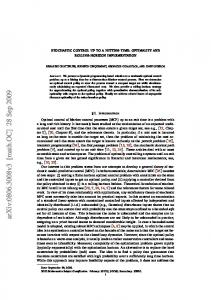
An example of a random disambiguation path. X = {x1 , x2 } consists of the centers of the two discs. . . . . . . . . . . . . . . . . . . . . . .

2.1 2.2

Illustration of a simplified DRDP instance with two discs. . . . . . . . Illustration of the partial AO tree corresponding to the DRDP instance illustrated in Figure 2.1. . . . . . . . . . . . . . . . . . . . . . . . . . 2.3 The BAO∗ Algorithm. . . . . . . . . . . . . . . . . . . . . . . . . . . 2.4 An experimental DRDP realization with |X| = 10. . . . . . . . . . . . 2.5 An experimental DRDP realization with |X| = 20. . . . . . . . . . . . 3.1 3.2 3.3 4.1 4.2 4.3 4.4 4.5 4.6 4.7

4.8 5.1 5.2

An example of a visibility graph. The dashed arcs graph edges since they are not in ∂(∪x∈X Rx ). . . . An example of a tangent arc graph. . . . . . . . . . Dijkstra’s Algorithm. . . . . . . . . . . . . . . . . .

are . . . . . .

not visibility . . . . . . . . . . . . . . . . . . . . . . . .

Marked point process realization. Gray-scale of discs reflects ρ of detections at respective disc’s centers. . . . . . . . . . . . . . . . . . . . All (two) possible realizations of pD2000 . . . . . . . . . . . . . . . . . . All (seven) possible realizations of pD100 . The probabilities are the respective probabilities of the path realizations. . . . . . . . . . . . . E`e pDα as a function of α, for c = 5. . . . . . . . . . . . . . . . . . . . E`e pDα for the optimal α, as a function of c. . . . . . . . . . . . . . . Nine realizations of a marked point process. . . . . . . . . . . . . . . Plots of E`e pDα against α = 2, 7, 12, 17, . . . for the respective nine realizations in Figure 4.6. Note that in each of these plots, for the largest value of α which is plotted, we have pDα = pD∞ . . . . . . . . . . . . Edge weights illustration with |X| = 4. . . . . . . . . . . . . . . . . . Illustration of an SDL with parallel avenues problem instance with three parallel avenues. . . . . . . . . . . . . . . . . . . . . . . . . . . An illustration of simulation environment A. . . . . . . . . . . . . . . x

8 22 23 28 30 32 39 41 44 54 55 56 57 59 62

63 66 79 84

5.3 5.4

An illustration of simulation environment B. . . . . . . . . . . . . . . An illustration of simulation environment C. . . . . . . . . . . . . . .

xi

85 85

List of Tables 2.1

Comparison of SDP, AO*, and BAO∗ on randomly generated DRDP instances. For |X| = 10, SDP did not run for either K due to excessive memory requirements. . . . . . . . . . . . . . . . . . . . . . . . . . .

4.1 x,y-coordinates and ρ’s for marked point process realization. . . . . . 4.2 All indifference intervals, the E`e pDα for values of α in the respective indifference intervals, and the range of disambiguation costs c where this indifference interval is optimal. For example, for any value 0 < c < 4.1013 the optimal value of α is any 26.77 < α < 30.23 and, as such, E`e pDα = 717.22 + 2.1665 c. . . . . . . . . . . . . . . . . . . . . 4.3 Weights of the edges in Figure 4.8. . . . . . . . . . . . . . . . . . . . 4.4 Comparison of E`ˆ p∗SR to E`p∗ . . . . . . . . . . . . . . . . . . . . . . . 5.1 5.2 5.3

Comparison of E`pCR to E`p∗ . . . . . . . Comparison of the CR and SR protocols example for different cost intervals. . . . Comparison of E`pCR to E`ˆ p∗SR . . . . . .

xii

. . on . . . .

. a . .

. . . . . . . . . . . . . mine countermeasures . . . . . . . . . . . . . . . . . . . . . . . . . .

31 54

59 67 68 82 83 86

Chapter 1 Introduction

1.1

Introduction

The research problem we consider in this dissertation, in its most broad setting, is a stochastic shortest path problem in the presence of a dynamic learning capability. Specifically, a spatial arrangement of possible obstacles needs to be traversed as swiftly as possible, and the status of the obstacles may be disambiguated (at a cost) en route. This problem has practical applications in important probabilistic path planning environments such as robot navigation in stochastic domains [15, 28, 45], mine countermeasures [70, 76], and adaptive traffic routing [27, 31]. No efficiently computable optimal policy is known for this problem, and many similar problems have been proven intractable. In this chapter, the research problem is defined in continuous and discrete settings and a comprehensive literature review is presented.

1

1.2

Continuous SDL

Suppose a decision maker (DM) needs to swiftly navigate from one given location to another through an arrangement of arbitrarily-shaped regions in the plane which are possible obstacles; at the outset the DM is given the respective probabilities that the regions are truly obstacles and, en route, when situated on a region’s boundary, the DM has the option to disambiguate the region, i.e., learn at a cost if the region is a true obstacle. We may sometimes assume that there is a limit on the number of available disambiguations. The central question is to find a policy (protocol)1 that decides what and where to disambiguate en route so as to minimize the expected length of the traversal. We call this problem the continuous Stochastic Shortest Path Problem With Dynamic Learning Capability (SDL), which is a minor modification of the Stochastic Obstacle Scene Problem (SOSP) of Papadimitriou and Yannakakis [55].

1.3

Discrete SDL

The discrete analogue of the above problem, which we call discrete SDL, is defined as follows: Let G = (V, E) be an undirected graph with designated vertices s, t ∈ V, 1

In this dissertation, we do not make any distinctions between a “policy” and a “protocol”, and we use the two terms interchangeably.

2

and suppose there is a function ` : E → R≥0 assigning a length to each edge; the goal here is to find a shortest s, t traversal (walk) in G. However, not all of the edges may indeed be traversable. In particular, for a given subset E0 ⊆ E of edges, called stochastic edges, there is a function ρ : E0 → [0, 1) such that, for each edge e ∈ E0 , ρ(e) is the probability that e is not traversable, independent of the other edges. (The edges in E \ E0 are known a priori to be traversable.) For any edge e ∈ E0 , when the traversal is at an endpoint of e, we have the option to disambiguate e—learning whether e is traversable—at a cost c(e) added to the length of the traversal, for some function c : E0 → R≥0 . Edges cannot be traversed until it is known that they are traversable, and, the traversability status of each edge is static and will never change over the course of the traversal.

Of course, if the DM follows any particular policy then the traversal is still random (and will unfold depending on the results of the disambiguations, so the traversal will have distribution specified through ρ). The goal, however, is to find an optimal policy in the sense of having shortest expected length. (As in the continuous version, we may sometimes assume that there is a limit K on the number of available disambiguations.) Finding such an optimal policy is the discrete SDL problem, which is known as the Canadian Traveler Problem (CTP) in the literature, and has been shown to be intractable [55]. To avoid infinite expected length, it may be helpful to assume the existence of a (possibly very long) s, t path consisting of edges from

3

{e ∈ E0 : ρ(e) = 0} ∪ (E \ E0 ).

Unless specified otherwise, we shall use the acronym “SDL” to collectively refer to both the continuous and discrete versions of the problem.

1.4

RDP

The main focus of this dissertation is on a variant of continuous SDL with disc-shaped possible-obstacles, called the Random Disambiguation Paths Problem (RDP) for historical reasons [29, 60]. In what follows, we describe the problem environment and formally define the RDP problem.

As in [60], consider a marked point process on a subset of R2 that generates random detections XT , XF ⊆ R2 (respectively called true and false detections), and, random marks ρT : XT → (0, 1] and ρF : XF → (0, 1]. When observing a realization of this process, the decision maker (DM) only sees X := XT

S

XF and ρ := ρT

S

ρF . We as-

sume that, for all x ∈ X, ρ(x) is the probability—conditioned on the observed values X and ρ—that x ∈ XT . It shall be assumed that the specific values of X and ρ have been observed and all discussion of probability is conditioned accordingly. We assume that whether or not any one x ∈ X is in XT is independent of any other x0 ∈ X. For every detection x, the possibly obstacle region Rx is an open disc centered at x with 4

radius r(x) > 0, for a given function r : X → R>0 . Given a starting point s ∈ R2 and a destination point t ∈ R2 , the DM seeks to traverse a continuous s, t curve in S ( x∈XT Rx )C of shortest achievable arclength.

Without any means of discovering which detections in X are true, the DM cannot S traverse any s, t curve shorter than the shortest s, t curve in ( x∈X Rx )C , denoted q(s, t, X). (The curve q(s, t, X) can be computed using the associated visibility graph described in Section 3.2). However, the DM has a dynamic capability of disambiguating detections from the boundaries of their associated discs. Specifically, when the DM is on ∂Rx for any x ∈ X, the DM can dynamically discover whether x ∈ XT or x ∈ XF , at a cost c(x) added to the Euclidean length of the curve, for a given cost function c : X → R≥0 . The DM is permitted to proceed through Rx only if x ∈ XF . There may also be a limit K on the number of available disambiguations. The DM’s goal is to minimize the traversal curve’s (expected) Euclidean length by efficiently exploiting the disambiguation capability.

A disambiguation protocol is a decision rule that specifies the DM’s actions under any circumstance and at any possible current location. Specifically, it is a function D that, to any such s, t, X, ρ, K, it assigns a detection x ∈ X and a point y ∈ ∂Rx (we explicitly allow y = t, in which case x is not defined). Given a disambiguation protocol D, the random disambiguation path pD is defined as the s, t curve in (∪x∈XT Rx )C

5

realized as follows: Suppose D associates x ∈ X and y ∈ ∂Rx to s, t, X, ρ, K. Then the DM is to traverse from s to y along a shortest path avoiding all the discs Rx0 such that x0 ∈ X is true or ambiguous. If y = t then terminate, otherwise disambiguate detection x (if K = 0 then it is required that y = t). The DM recursively repeats this entire procedure using y in place of s, updating X and ρ as follows: If the disambiguation has just discovered that x ∈ XT then update ρ(x) := 1, and if the disambiguation has just discovered that x ∈ XF then remove x from X; either way, decrement K by 1 (if indeed there is a limit on the number of available disambiguations).

The random disambiguation path pD is an s, t-curve-valued random variable even after X and ρ are observed since the emerging outcomes of the disambiguations dictated by the protocol are still random. In fact, the distribution of pD is specified through ρ.

The Random Disambiguation Paths Problem (RDP) is then defined as choosing the disambiguation protocol—among all possible disambiguation protocols—that minimizes the expected total traversal length.

To illustrate, suppose K = 2 and s, t, X, ρ are as shown in Figure 1.1, and consider one particular disambiguation protocol D which, say, dictates that the next (i.e., first) disambiguation be of detection x1 at point y1 . Now suppose, if it is discovered that

6

x1 ∈ XF , D would then dictate that no more disambiguations be performed, and the curve should proceed to t. Also suppose, if it is instead discovered that x1 ∈ XT , D would then dictate that x2 should be disambiguated next, at point y2 . Whether x2 is revealed to be a true or false detection, D would then dictate that the DM proceeds directly to t, since no more disambiguations are available (currently K = 0). There are three possible realizations of the random disambiguation path pD , each pictured in Figure 1.1:

• With 1 − ρ(x1 ) = .7 probability, pD traverses the points s, y1 , t; • With ρ(x1 )ρ(x2 ) = .27 probability, pD traverses the points s, y1 , y2 , t employing the curve γ at the traversal conclusion; and, • With ρ(x1 )(1 − ρ(x2 )) = .03 probability, pD traverses the points s, y1 , y2 , t employing the line segment y2 , t at the traversal conclusion. Note that in between disambiguations the s, t curve traverses the shortest curves avoiding all possibly forbidden risk regions—using the corresponding visibility graphs. If the lengths of these three paths are, respectively, 6, 8, 7, and if the cost of disambiguation was c = 5 then then the expected length of pD is given by (1 − .3)(6 + 1 ∗ 5) + (.3)(.9)(8 + 2 ∗ 5) + (.3)(1 − .9)(7 + 2 ∗ 5).

In the above example, we illustrated one particular disambiguation protocol D; a different choice of protocol may indeed yield a significantly lower expected length. 7

Figure 1.1: An example of a random disambiguation path. X = {x1 , x2 } consists of the centers of the two discs.

1.5

Discrete RDP

Optimal disambiguation protocols are not readily computable for all but the most trivial instances of RDP. We therefore consider a discrete approximation which is, for simplicity and convenience, on a subgraph of the integer lattice Z2 . Specifically, it is the graph G whose vertices are all of the pairs of integers i, j such that 1 ≤ i ≤ imax and 1 ≤ j ≤ jmax , where imax and jmax are given integers. There are edges between all pairs of vertices of the form (i, j) and (i + 1, j), and there are edges between all pairs of vertices of the form (i, j) and (i, j + 1). One vertex in G is designated as the starting point s, another vertex in G is designated as the termination point t, and the decision maker is to walk from s to t in G, only traversing edges that do not intersect any true or ambiguous obstacles. If an edge intersects any ambiguous obstacle, then a disambiguation of the obstacle may be performed from either of the

8

edge’s endpoints that is outside of the obstacle. As before, the goal is to develop a policy that minimizes the expected length of the traversal by effective exploitation of the disambiguation capability. We call the discretized version as the Discrete RDP (DRDP), which, in effect, is a special case of discrete SDL (and CTP) with statistical dependency among the edges.

1.6

Literature Review

The shortest path problem in deterministic networks—where each arc has a fixed, known length—is widely encountered in theory as well as practice and has been wellstudied. Various efficient algorithms exist for solving such problems and a traditional treatment of this subject can be found in [1, 22].

In many practical applications, however, arclengths are not known in advance and it can be more realistic to model them as random variables, which gives rise to stochastic shortest path problems. A particular version of this class of problems is the one with a dynamic learning capability, where the realization of arclengths is learned as the traversal progresses. A wide variety of such problems have been studied, including arc-wise and time-wise dependencies [21, 24, 30, 49, 73]. Most of these studies were conducted by researchers in the disciplines of transportation science [8, 20, 27, 42], computer science (theoretical computer science and artificial intelli9

gence) [9, 15, 28, 45, 55], and operations research [6, 7, 12, 23, 59, 63]. The work in these three communities was done, by and large, independent of each other.

The continuous SDL problem is a minor modification of the Stochastic Obstacle Scene Problem (SOSP) of Papadimitriou and Yannakakis [55], where possibly intersecting rectilinear blocks may be present in an obstacle scene and whether a specific block exists or not can be learned only by visual contact. The authors also describe a discrete version of this problem called the Canadian Traveler Problem (CTP), which we refer to as discrete SDL in this dissertation. Papadimitriou and Yannakakis prove the intractability of several variants of SOSP and CTP. Several modifications and extensions of CTP are discussed in [9], [15], and [45]. Baglietto et al. [7] cast CTP as a stochastic optimal control problem and propose a heuristic method based on neurodynamic programming. Ferguson, Stenz, and Thrun [28] also propose a heuristic for CTP, which is a more elaborate version of the AO∗ Algorithm.

CTP is a special case of the Stochastic Shortest Paths with Recourse (SPR) problem of Andreatta and Romeo [6], who present a stochastic dynamic programming formulation for SPR and note its intractability. Polychronopoulos and Tsitsiklis [59] also present a stochastic dynamic programming formulation for SPR and then prove the intractability of several variants. Provan [63] proves that SPR is intractable even if the underlying graph is directed and acyclic.

10

The underlying difficulty in obtaining a tractable stochastic dynamic programming formulation of these problems—even in the discrete setting—is that in order for the actions to be considered at any given location, there is a need to know the current ambiguous/true/false status of all of the detections, and the exponentially many such possibilities need to be incorporated accordingly.

1.7

Organization of the Dissertation

The rest of this dissertation is organized as follows:

Chapter 2 casts SDL as a Markov Decision Process and introduces the BAO∗ Algorithm for DRDP, which is not polynomial-time, but can be used to optimally solve relatively small instances of the problem. This chapter also formulates RDP as a Partially Observable Markov Decision Process.

Chapter 3 discusses visibility graphs and introduces the tangent arc graph data structure, which plays an important role in the next chapters. This chapter also points out that the well-known A∗ Algorithm with a slightly stronger admissibility requirement on the heuristic function is equivalent to Dijkstra’s Algorithm under a change of variable. 11

Chapter 4 presents the simulated risk disambiguation protocol (SR) for RDP and DRDP, which is suboptimal, but efficiently computable as well as reasonably effective.

Chapter 5 introduces the CR disambiguation protocol for RDP and DRDP, which is also suboptimal, but much more efficiently computable even than SR, and, as illustrated via simulations, yields solutions that compare favorably to those obtained by the optimal policy and also SR. The chapter proves optimality of the CR protocol for parallel graphs in the discrete setting. This chapter also shows that the situation where there is an obstacle neutralization capability instead of the disambiguation capability can be seen as a special case of the setting that leads to the CR protocol.

Chapter 6 presents summary, conclusions, and directions for future research.

12

Chapter 2 The BAO∗ Algorithm

2.1

Introduction

In this chapter, we first cast SDL as a Markov Decision Process and develop the corresponding Bellman equation, whose solution via stochastic dynamic programming can yield the optimal policy. However, the state space is too large to efficiently utilize the dynamic programming paradigm. Next, we define AO trees, which can be used to allow partial solutions of the optimality conditions to be selectively searched—without exhaustively back-solving complete stages as in stochastic dynamic programming. In particular, the well-known AO∗ Algorithm was devised for searching AO trees. Introduced in Section 2.3 is a new improvement on AO∗ that we call the BAO∗ Algorithm, which employs stronger pruning methods, including the utilization of both upper and lower bounds on path lengths, and significantly speeds up the search process. The

13

chapter concludes with a Partially Observable Markov Decision Process formulation of RDP.

2.2

Markov Decision Process Formulation

A Markov Decision Process (MDP) is a mathematical framework for modeling sequential decision-making processes in an environment with the Markov property, i.e., the complete past history is summarized in the current state. At discrete time steps called stages, a decision maker (DM) is at a state contained in a state space, at which he chooses an action from a set of actions and earns a reward that depends on the current state and the action chosen. The state arrived at the next stage is probabilistic and the distribution depends only on the current state and the action chosen. The DM’s goal is to maximize the expected sum of rewards earned over all stages, sometimes with a discount factor on future rewards. It is assumed that the DM knows his current state at all times. An in-depth discussion of MDPs can be found in [64, 74].

Formally, an MDP is a 4-tuple < S, A, T , R > where

• S is a set of states: At every stage k = 0, 1, 2, . . . , K (where K is the final stage, or K = ∞), the DM is at one of these states; • A is a set of actions: At every stage, the DM chooses one of them depending 14

on what his current state is; • T : S × A × S → [0, 1] is the state-transition function: For any s, s0 ∈ S and α ∈ A, T (s, α, s0 ) is the probability of ending up in state s0 in the next stage given that the DM is at state s in the current stage and chooses action α; and, • R : S ×A → R is the reward function: R(s, α) represents the immediate reward the DM gains for choosing action α at state s.

The DM’s objective is to maximize the expected sum of rewards (possibly discounted by a factor λ ∈ (0, 1], i.e., E

 PK

k=0

 λk Rk where Rk is the reward received at stage k).

We now simultaneously cast continuous and discrete SDL as a finite-horizon MDP (i.e., K < ∞), formulating the components of < S, A, T , R > as follows.

• States: Let N be the number of possible-obstacles in the continuous setting, and the number of stochastic edges in the discrete setting. In order to keep track of the decision maker’s current knowledge of the status of possible-obstacles (or stochastic edges), we define the information vector I ∈ {“A”,“T”,“F”}N , such that, for all i = 1, 2, . . . , N , the i-th entry of I is “A”, “T”, or “F”, according as the current status of i-th possible-obstacle (or stochastic edge) is ambiguous, true, or false, respectively.

15

Let Y be the union of s, t, and the set of all disambiguation locations, i.e., locations at which possible-obstacles (or stochastic edges) can be disambiguated. (In continuous SDL, these locations are points on the plane and, in discrete SDL, they are vertices in the underlying graph.) If there are certain locations at which multiple possible-obstacles (or stochastic edges) can be disambiguated, these locations are included in Y with their respective multiplicities.

The MDP state space S is defined as Y × {“A”,“T”,“F”}N . The state space thus represents possible locations at which the DM may be at a particular stage, coupled with information that describes the decision maker’s knowledge at that stage.

• Actions: The set of actions A is Y\{s}, i.e., all the locations where a disambiguation can be performed and the destination.

• State Transition Function:

Given a state and an action, the state transi-

tioned into is comprised of the location identified in the action and, the information vector of the previous state updated to indicate whether the possibleobstacle (or stochastic edge) identified in the action is true or false; with respective probabilities being specified according to its mark.

16

• Rewards: The reward for a specific action at any particular state is the negative of the shortest path distance between the location identified in the state and the location identified in the action—avoiding all ambiguous and true obstacles (or stochastic edges) as indicated by that state’s information vector. The disambiguation cost is also subtracted if the location identified in the action is not the destination.

The above state space, set of actions, rewards, and state transition function comprise a Markov Decision Process with K stages (or N stages if there is no limit on the number of available disambiguations).

We now present the Bellman equation corresponding to the above MDP formulation, which can be solved via standard stochastic dynamic programming (SDP) for relatively small instances in the discrete setting. The reader is referred to [10, 11, 51] for a general discussion of dynamic programming and [67] for an introduction to stochastic dynamic programming. The notation used in the Bellman equation is as follows. • For s = (y, I) ∈ S and stage k ≤ K, the value function Vk∗ : S → R is defined as the negative of the shortest expected y, t path length under an optimal policy when the status of the obstacle field (or the underlying graph) is I, and there

17

are k disambiguations left. • For any y, y 0 ∈ Y and information vector I, q(y, y 0 , I) is defined as the length of the shortest y, y 0 path while avoiding all the true and ambiguous obstacles (or stochastic edges) as indicated by I. • For any y ∈ Y, Iy is defined as the component of I corresponding to the possible-obstacle (or stochastic edge) associated with y. • For any y ∈ Y, ρ(y) is defined as the mark of the possible-obstacle (or stochastic edge) associated with y. • For information vector I and y ∈ Y, TI,y and FI,y are defined as the information vectors whose components are the same as I except at the component corresponding to y, which is set to “T” and “F”, respectively. For k = 1, . . . , K, and s = (y, I) ∈ S, the Bellman equation is as follows:

Vk∗ (s) =

max 0

y ∈Y s.t. y 0 =t or Iy0 =“A”



∗ − q(y, y 0 , I) − δy0 6=t · c + ρ(y 0 )Vk−1 (y 0 , TI,y0 )

∗ + (1 − ρ(y 0 ))Vk−1 (y 0 , FI,y0 )

(2.1)

where δ is the indicator function. The optimal solution to SDL is then given by −VK∗ ((s, (“A”,. . . ,“A”))). Note that an SDP solution entails exhaustively back-solving complete stages from stage 1 up to stage K, where stage 0 values V0∗ ((y, I)) are given

18

by −q(y, t, I).

For continuous SDL, the above SDP approach is not practically applicable due to the infinitely many states and actions—yet they provide valuable insight into the structure of this class of problems and illustrate their difficulty. Due to exponentially many states, the SDP approach is not practical for discrete SDL either, as illustrated in the computational experiments of Section 2.4.

2.3

The BAO∗ Algorithm

In this section, we first define AO trees, which can be used to represent a given DRDP instance as a rooted tree with exponentially many nodes—the branches of the tree correspond to sequential decisions that can be made and their probabilistic outcomes. We next describe the AO∗ Algorithm for searching AO trees, and introduce the BAO∗ Algorithm [2], which stands for AO∗ with bounds. The BAO∗ Algorithm improves upon AO∗ by utilizing stronger pruning techniques and speeds up the search process significantly.

19

2.3.1

AO Trees

An AO tree is defined as a rooted tree T = (N, A) with a function ` : A → R≥0 assigning a length to each arc, and a function p : A → [0, 1] assigning a probability to each arc. The node set N is partitioned into a set of AND nodes, denoted by NA , and a set of OR nodes, denoted by NO . All arcs emanating from OR nodes have probability one. AO trees are the AND-OR graphs commonly found in the literature, see e.g., [52].

Denote by S(n) the successors of the node n ∈ N in the AO tree. A function g : N → R≥0 is said to be consistent on a collection of nodes C ∈ N provided that, for all n ∈ C, the following three conditions are satisfied: • if n ∈ NA , g(n) =

P

n0 ∈S(n)

  p(n, n0 ) · (`(n, n0 ) + g(n0 )) ,

• if n ∈ NO , g(n) = minn0 ∈S(n) {`(n, n0 ) + g(n0 )}, and, • if n ∈ N is a leaf node, g(n) is zero. The function f : N → R≥0 that is consistent on N is called the cost-to-go function and f (n) is called the true label 1 of node n. Typically, ` and p are given explicitly, and f is implicitly defined via ` and p. Given an AO tree, the goal is to compute the true label of the root node, which denotes the optimal value of an underlying decision problem.

1

In our context, f will denote the negative of the SDP value function V ∗ defined in Section 2.2.

20

A DRDP instance can be solved by computing the true label of the root node of an appropriately chosen AO tree. Specifically, associated with each node n is a state sn = (yn , In ) from the state space S = Y × {“A”,“T”,“F”}|X| . The root r is an OR node with yr = s and Ir = (“A”, . . . , “A”), which is the first generation in the tree. All subsequent odd generations consist of OR nodes corresponding to possible disambiguation locations, and even generations consist of AND nodes which are either leaf nodes denoting direct traversal to destination, or, have two successors each of whom corresponds to true and false disambiguation outcomes. For any arc a = (n, n0 ) ∈ A,

• If n ∈ NO , `(a) is set to q(yn , yn0 , In ) and p(a) is set to one. • If n ∈ NA , `(a) is set to the disambiguation cost c and, p(a) is set to ρ(yn ) if n0 corresponds to a true disambiguation outcome and 1 − ρ(yn ) otherwise.

Note that the same state could be associated with multiple nodes in the AO tree. This construction is essentially a mapping of all the actions the DM can choose and all the disambiguation outcomes that can occur. In particular, this construction ensures that f (n) is the negative of V ∗ (sn ) for any node n ∈ NO .

As an example, consider the DRDP instance in Figure 2.1 with two discs centered at (3, 2) and (6, 2) respectively, with s = (1, 2) and t = (8, 2). For simplicity, we assume that each disc can be disambiguated only at the point to its left, i.e., the first disc 21

can be disambiguated at y1 = (2, 2) and the second at y2 = (5, 2).

Figure 2.1: Illustration of a simplified DRDP instance with two discs.

A partial AO tree corresponding to this instance, for K = 2, is illustrated in Figure 2.2, where the successors of the node (y2 , (“A”, “A”)) are not shown. AND nodes are depicted by circles and OR nodes by squares. The numbers next to each arc denote its length and thick-bordered circles represent leaf nodes.

In an AO tree representation of DRDP, the optimal disambiguation protocol is a collection C of all the arcs whose lengths are explicitly included in the calculation of f (r). Specifically, we first define the function m : NO → NA such that m(n) := arg minn0 ∈S(n) {`(n, n0 )+f (n0 )} for any n ∈ NO . We identify the collection C recursively as follows:

22

Figure 2.2: Illustration of the partial AO tree corresponding to the DRDP instance illustrated in Figure 2.1.

23

Step 1. Set C := ∅ and nm := r. Step 2. If m(nm ) is a leaf node, augment C by (nm , m(nm )). Otherwise, augment C by (nm , m(nm )), (m(nm ), n0 ), and (m(nm ), n00 ) where n0 and n00 are the successors of (m(nm )). Step 3a. Set nm := n0 . If nm is not a leaf node, go to Step 2. Step 3b. Set nm := n00 . If nm is not a leaf node, go to Step 2.

The benefit of the AO tree representation is that, as shown in Section 2.3.2, it allows for selectively evaluating the value function in a top-down fashion rather than back-computing all of them for every stage as in the dynamic programming paradigm.

2.3.2

The AO∗ Algorithm

Theoretically, an optimal solution to a problem represented by an AO tree can be determined by computing f (n) for all n ∈ N in a bottom-up fashion. However, the exponential number of nodes in the AO tree representation of DRDP makes this approach prohibitively expensive. On the other hand, not all the nodes’ true labels need to be calculated to determine the true label of the root node. We define searching an AO tree as identifying the nodes that are of interest in determining the true label of the root node.

24

The classical AO∗ Algorithm for searching AO trees [18, 48, 52] improves upon the brute force approach by utilizating admissible bounds h : N → R≥0 , called heuristic labels, which are lower bounds that are guaranteed not to overestimate the true label of any node. These lower bounds guide the search in a top-down fashion so that only a small portion of the complete AO tree is examined. The AO∗ Algorithm and its variants have been used by researchers to successfully solve various decision problems [8, 28, 52]. The AO∗ Algorithm is described below.

The AO∗ Algorithm grows a solution tree S = (N0 , A0 ), which is a subtree of the complete AO tree and a representation of partial solutions of the optimality conditions. S initially consists of only the root node r, and is gradually augmented by two alternating steps, expansion and propagation, until f (r) is computed. A node n0 ∈ N0 is said to be terminal if f (n0 ) has been calculated. In the expansion step, the non-terminal leaf node with the lowest h value, called the expansion node and denoted by n0e , is found and its successors are added to S. The successors are then are assigned heuristic labels. In the propagation step, h(n0e ) is recalculated using the labels of its successors—true labels for successors that are leaf nodes in the complete AO tree and heuristic labels otherwise—and the new label is propagated up S until a node is reached whose heuristic label is not affected. Terminal status of nodes are also updated accordingly during the propagation step.

25

In DRDP, an admissible lower bound on f (n) for any n ∈ N is available in the form of the shortest path length from yn to destination while avoiding only the true stochastic edges as indicated by In —which allows for the use of the AO∗ Algorithm to solve relatively small instances of the problem.

2.3.3

BAO∗

An important characteristic of the DRDP problem is that the expected length of the optimal protocol is always upper bounded by the zero-risk s, t traversal. In this section, we present an improvement on AO∗ that incorporates this additional information and significantly speeds up the search, which we call BAO∗ for AO∗ with bounds.

The BAO∗ Algorithm intelligently incorporates the lower and upper bound information described above and examines only a very small fraction of the complete AO tree to compute the true label of the root node. BAO∗ is not polynomial-time, but it can substantially shorten the running time needed to find an exact solution to small instances. As illustrated in the computational experiments section, BAO∗ has significant computational savings over SDP and AO∗ . BAO∗ pseudocode is presented in Figure 2.3.

Key features and benefits of BAO∗ are as follows:

26

Algorithm BAO∗ Input: DRDP instance. Output: Minimum expected traversal length from s to t. Begin 1. Set zeroRiskDist := q(s, t, (“A”,. . . ,“A”)). 2. Generate node root with state (s, (“A”,. . . ,“A”)). 3. While (root is not marked as terminal) Begin % Identify the node to be expanded: 3.1. Set totalPathDist := 0. 3.2. Set expandNode := root. 3.3. While (expandNode != null) Begin 3.3.1. If expandNode is a non-leaf AND node, lower bound the heuristic label of its true successor by h(expandNode). 3.3.2. Set totalPathDist += expandNode’s distance from its parent in the parent’s information state. 3.3.3. Set expandNode := expandNode’s best non-terminal successor. End while % Expand best partial solution: 3.4. Temporarily generate the AND node (t, expandNode’s information state). If its total s, t traversal length is less than zeroRiskDist, add it to expandNode’s successors list. 3.5. If there are any disambiguations left, temporarily generate AND nodes corresponding to each disambiguation location of ambiguous stochastic edges that are reachable in expandNode’s information state. Also generate true and false OR successors for them. 3.6. Compute the heuristic labels of these OR nodes, htrue and hf alse , respectively, and set heuristic label of the parent AND node to hweighted = ρ · htrue + (1 − ρ) · htrue , where ρ is the mark of the disc associated with this node. 3.7. For each of the AND nodes, compute a heuristic s, t traversal length as htotal := totalPathDist + (distance to expandNode in expandNode’s information state) + hweighted . If htotal < zeroRiskDist, add these AND nodes to expandNode’s successors list and also their two successors. Otherwise, delete them. If there is only one disambiguation left, generate the AND node’s two successors and compute their true labels. Also mark this AND node as terminal.

27

%Propagate new labels and update the solution tree: 4. Set continueProp := true. 5. While (continueProp) and (expandNode != null) do Begin 5.1. If expandNode is an OR node and it does not have any successors, mark it terminal. Otherwise, search the successors of expandNode’s parent and find the node that yields the lowest heuristic label. Update the parent’s best successor node and the parent’s heuristic label. 5.2. If expandNode is a non-leaf AND node, set h(expandNode) to the weighted average of the heuristic labels of its two successors. Update the best non-terminal successor of the parent of expandNode. If the parent node does not have any non-terminal successors, mark it terminal. 5.3. If the new h(expandNode) plus the distance between expandNode and the root is not less than zeroRiskDist, then delete expandNode and all of its successors. 5.4. Set continueProp := false if the heuristic label of expandNode has not changed. 5.5. Set expandNode := expandNode’s parent. End while End while End Figure 2.3: The BAO∗ Algorithm.

28

1. BAO∗ only expands OR nodes. Successor AND nodes and an AND node representing direct traversal to the destination are automatically generated, but only when the heuristic s, t traversal lengths of these nodes are less than the conventional zero-risk s, t path. 2. BAO∗ lower bounds the heuristic label of true OR nodes by the heuristic labels of their parents as it moves down the solution tree during the expansion step; providing better estimates. 3. If there is only one disambiguation left at the current expansion node, the true label of the expansion node is calculated and the corresponding AND node is marked as terminal. This feature eliminates the overhead cost of individually considering the successors of this AND node in future expansions. 4. As the updated labels are propagated up the solution tree, new node labels are used to dynamically delete the nodes whose heuristic s, t traversal lengths exceed the length of the zero-risk s, t path. A variant of the AO∗ Algorithm is discussed in [28], which propagates heuristic labels across to neighbors in the complete AO tree during the propagation process. However, the exponentially many nodes in DRDP representation renders this approach impractical and we do not incorporate this logic in BAO∗ .

29

2.4

Computational Experiments

In this section, we compare the performances of SDP, AO*, and BAO∗ on relatively small, but non-trivial DRDP instances. For all of the experiments, imax is taken as 20 and jmax is taken as 15 on the integer lattice, with s = (10, 15) and t = (10, 1). Each possible-obstacle is a disc with radius 2.5, with their centers sampled from a uniform distribution on the pairs of real numbers in [4, 17] × [4, 12]; in particular, this ensures that there is always a permissible path from s to t. Marks of the discs are sampled from a uniform distribution on the unit interval. Throughout the simulations, the disambiguation cost c is taken as 3.0. The simulation environment is illustrated in Figure 2.4 for |X| = 10 where the dark-colored edges represent stochastic edges.

Figure 2.4: An experimental DRDP realization with |X| = 10.

30

Table 2.1 compares the performances of SDP, AO*, and BAO∗ for 20 experiment realizations for each |X|, K combination listed. The third, fourth, and fifth columns in the table show the average execution times of SDP, AO*, and BAO∗ respectively, on a 3.5 gigahertz personal computer with 1 gigabyte memory. SDP did not run for |X| = 10 for either K due to insufficient memory. The next column displays the mean number of value function evaluations in SDP. The last two columns show the mean number of nodes expanded by AO∗ and BAO∗ , respectively.

|X| = 7 |X| = 10

K K K K

=1 =2 =1 =2

Mean execution time SDP AO∗ BAO∗ 19.0s 7.1s 5.4s 4.2m 22.1m 1.9m — 9.0s 7.3s — 33.1m 2.8m

Mean # of V ∗ calc’s in SDP 1677 10,841 — —

Mean # of expansions AO∗ BAO∗ 119 31 12,653 322 128 41 15,052 386

Table 2.1: Comparison of SDP, AO*, and BAO∗ on randomly generated DRDP instances. For |X| = 10, SDP did not run for either K due to excessive memory requirements.

As shown in Table 2.1, mean AO∗ and BAO∗ runtime were less than that of SDP for |X| = 7, K = 1. However, since the same state can reside in multiple nodes in the AO tree when K > 1, the number of AO∗ expansions can exceed the number of value function evaluations in SDP, causing AO∗ runtime surpass SDP runtime, as illustrated for |X| = 7, K = 2. On the other hand, for K = 2, the mean number of node expansions in BAO∗ was only about 2.5% of the mean number of expansions in AO∗ , for both |X| = 7 and |X| = 10. For |X| = 10, SDP did not run even for K = 1

31

due to excessive memory requirements, whereas BAO∗ mean runtime for K = 2 was just 2.8 minutes, which was only 8.5% of the mean AO∗ runtime, illustrating the efficiency of the BAO∗ Algorithm in solving small DRDP instances.

Figure 2.5: An experimental DRDP realization with |X| = 20.

To further illustrate the efficiency of BAO∗ on relatively small DRDP instances, we conducted a second set of simulations where imax = 20 and jmax = 15, with s = (10, 15) and t = (10, 1), as above. This time, disc radii are set to 1.5 and the disc centers are sampled from a uniform distribution on the pairs of real numbers in [3, 18] × [3, 13]. Number of discs is taken as 20 and the cost of disambiguation is taken as 1.5. Disc marks are sampled from a uniform distribution on the unit interval. The simulation environment is illustrated in Figure 2.5. For 10 experiment realizations in

32

this environment with K = 2, mean BAO∗ execution time was just 7.4 minutes and mean number of node expansions was 1,957. On the other hand, mean AO∗ execution time was 2.7 hours whereas mean number of node expansions was 43,309. We did not perform additional simulations with K = 3 as one such run of BAO∗ took almost 20 hours.

2.5

Partially Observable Markov Decision Process Formulation

A Partially Observable Markov Decision Process (POMDP) is a generalization of the MDP framework where the decision maker (DM) no longer has direct access to his current state, but instead, has the ability to make observations via imperfect sensors. MDPs can handle uncertainty regarding the outcomes of the DM’s actions, whereas POMDPs can also cope with uncertainty arising from lack of complete state knowledge as well as uncertainty due to imperfect sensing [40, 72]. MDPs can be solved in polynomial-time [50, 77], whereas POMDPs have been shown to be intractable and are difficult to solve in general [54].

A POMDP is denoted as a 6-tuple < S, A, T , R, Ω, O > where

• S, A, T , and R denote a Markov Decision Process; 33

• Ω is a set of observations the DM can make; and, • O : S × A × S × Ω → [0, 1] is the observation function: For each current state, action, and resulting state, it specifies a probability distribution over possible observations. Specifically, O(s, α, s0 , o) is the probability of observing o when the DM is at state s, chooses action α, and ends up in state s0 .

As shown below, RDP can be cast as a POMDP by trimming the set of information vectors to {“T”,“F”}|X| and, folding the ambiguity of detections into ambiguity of the information vector, hence the partial observability of the state. Current POMDP technology is not sufficient to efficiently solve RDP in this manner [69], but, this formulation keeps open more options for attacking the problem in the future. In our formulation, we shall assume that cost of disambiguation is zero and there is no limit on the number of available disambiguations. The motivation for this assumption is that the reward for each state/ action pair needs to be specified a priori and, the DM may have to re-disambiguate certain detections in order to traverse the shortest path used to calculate this reward. We formulate the components of < S, A, T , R, Ω, O > as follows2 : • States: The POMDP information vector is defined as I 0 ∈ {“T”,“F”}|X| such that, for all i = 1, 2, . . . , |X|, the i-th entry of I 0 is “T” or “F”, according as the actual status of i-th detection is true or false. For each disambiguation 2

This formulation can be generalized to continuous and discrete SDL in a relatively straightforward manner.

34

location y ∈ Y, we introduce two points: yout that is an exact copy of y (called an out-point), and yin that is y infinitesimally perturbed from its location into the interior of the associated disc (called an in-point)—yin cannot be arrived at unless the associated detection is false. Let Y 0 be the union of s, t, and, the in- and out-points associated with each disambiguation location. The POMDP state space is defined as Y 0 × I 0 . We shall refer to the location component of a given state as the state point. • Actions: The set of actions is Y 0 \{s}. • State Transition Function: Given a state and an action, the state point of the state transitioned into is the point as identified by the action. The information vector of state transitioned into is always the same as the information vector of the current state. • Rewards: At any state whose state point is an out-point, the reward for choosing the corresponding in-point as the action is 0 if the detection associated with them is false, and −∞ otherwise. For any other state/ action pair, the reward is the negative of the shortest path distance between the state point and the action avoiding all the discs (regardless of the actual status of their associated detections) except the ones that the DM is currently inside of. • Observations: The set of observations Ω is {true, false}. • Observation Probabilities: Since state transitions are always deterministic, 35

the observations only need to be specified for state/ action pairs, which are true or false according as the actual status of the detection associated with the actions.

Thanks to the assumption that the cost of disambiguation is zero and there is no limit on the number of available disambiguations, the DM can traverse through discs that have been previously disambiguated by re-disambiguating them whenever they need to be re-traversed.

Notice that in the above formulation, state transitions and observations are deterministic and, all the ambiguity is folded into the information vector. The information vector, on the other hand, represents the DM’s current knowledge of the obstacle field, whose probability distribution (called the belief state in POMDP terminology) is specified by the disc marks.

36

Chapter 3 Data Structures

3.1

Introduction

In this chapter, we first discuss visibility graphs, which can be used to to compute deterministic shortest paths through arrangements of definite-obstacles in the plane. Then, we introduce the tangent arc graph (TAG) data structure, which is the topological superimposition of all of the visibility graphs generated by the collection of all subsets of obstacles. Even though there are exponentially many such subsets, the TAG is polynomially-sized. The TAG plays a fundamental role in the protocols developed for RDP in the next two chapters. We then point out that the well-known A∗ Algorithm with a slightly stronger admissibility requirement on the heuristic function is equivalent to Dijkstra’s Algorithm under a change of variable. Such a heuristic function is available for tangent arc graphs with the various edge weights our protocols

37

use, and this will speed up finding shortest paths as part of computing these protocols.

3.2

The Visibility Graph

The visibility graph is a data structure that can be used to find deterministic shortest paths through arrangements of definite-obstacles in the plane. In particular, visibility graphs can be used to compute q(s, t, X), the shortest zero-risk path from s to t associated with X in RDP. Our visibility graph is an adaptation of the visibility graph from [47] and [66], more similar to the generalized visibility graph in [65]. The visibility graph is also used in the formation of the tangent arc graph, another important data structure presented in the next section.

Let s, t and X be specified.

For any distinct points a, b ∈ {s, t}

S

∂(∪x∈X Rx ),

we call the closed line segment a, b a tangent segment provided that (1) for all r ∈ {a, b}\{s, t}, a, b is tangential to ∂(∪x∈X Rx ) at r and (2) the relative interior of a, b is contained in the interior of [(∪x∈X Rx ) ∪ {s, t}]C .

The visibility graph associated with s, t, X is defined as follows. Its vertex set consists of s, t, all points of ∂(∪x∈X Rx ) which intersect a tangent segment, and all points of ∂(∪x∈X Rx ) at which two or more ∂Rx ’s intersect. The edge set of the visibility graph consists of all tangent segments and all connected components of ∂(∪x∈X Rx ) 38

after the vertices of the visibility graph are removed (the latter edges are segments of arc from circles). The graph theoretic endpoints of these edges are their line and arc endpoints, respectively, and each edge is weighted with its arclength. An example of a visibility graph is pictured in Figure 3.1.

Figure 3.1: An example of a visibility graph. The dashed arcs are not visibility graph edges since they are not in ∂(∪x∈X Rx ).

It is a well-known (and true) folk theorem that q(s, t, X) is the shortest s, t path in the visibility graph associated with s, t, X. Since every pair of nonidentical ∂Rx ’s have at most 4 mutually tangential lines and two points of intersection, the number of vertices and edges in the visibility graph are each O(|X|2 ). Thus Dijkstra’s algorithm with a heap implementation [1] applied to this visibility graph yields q(s, t, X) in O(|X|2 log |X|) operations. For each pair of nonidentical ∂Rx ’s, O(|X|) ∂Rx ’s need to be checked for intersection with the tangential lines associated with this pair, thus

39

the naive construction of the visibility graph can be accomplished in O(|X|3 ) assignment, arithmetic, and trigonometric operations.

3.3

The Tangent Arc Graph

The tangent arc graph (TAG) is a new data structure comprised of the topological superimposition of all the visibility graphs generated by the collection of all subsets of disc-shaped obstacles. Although there are exponentially many such subsets (hence exponentially many such generated visibility graphs), the TAG is polynomially-sized, as described below.

Given s, t, X, and ρ, for any distinct points a, b ∈ {s, t} ∪

S

x∈X


∂Rx , we say

the closed line segment a, b is a general tangent segment provided that, for all r ∈ {a, b}\{s, t}, a, b is tangential to ∂Rx for some x ∈ X. The TAG is defined as follows: The vertex set of TAGs,t,X consists of s, t, all points of intersection between any general tangent segment and any ∂Rx (over all x ∈ X), and all points of intersection between two or more ∂Rx ’s. The edge set of TAGs,t,X consists of all connected components of all general tangent segments after the vertices of TAGs,t,X are removed, and all connected components of ∪x∈X ∂Rx after the vertices of TAGs,t,X are removed.

An example of a TAGs,t,X is pictured in Figure 3.2. In this example, there are 11 40

general tangent segments; in particular, one of these is the line segment s, t, which intersects boundaries of discs in two places. These two intersections become vertices in TAGs,t,X and, upon removal from s, t, three TAGs,t,X edges are created in s, t’s place. In total, this TAGs,t,X has 21 vertices and 37 edges; 16 of these edges are line segments and 21 of these edges are segments of arc from circles.

Figure 3.2: An example of a tangent arc graph.

Note that the graph TAGs,t,X is a topological superimposition of all the visibility graphs generated by s, t, Y over all Y ⊆ X. There are O(|X|2 ) general tangent segments, each intersecting O(|X|) regions of the form Rx : x ∈ X, so we have O(|X|3 ) vertices and O(|X|3 ) edges in TAGs,t,X . Thus, shortest paths in TAG may be found in O(|X|3 log |X|) operations by using a heap implementation of Dijkstra’s Algorithm. Since the O(|X|) regions intersecting the general tangent segments can be sorted in O(|X| log |X|), the number of operations to set up TAG is O(|X|3 log |X|). 41

An important feature of TAG is that any shortest path in the plane restricted to avoid any subset of the original obstacles will automatically be in TAG regardless of which subset of obstacles are to be avoided. Consequently if, rather than obstacles being untraversable, there is an additive ”penalty” (added to traversal length) for traversing the respective obstacles, then a shortest path in this setting will also be in TAG.

3.4

The A∗ and Dijkstra’s Algorithms

The protocols we introduce for RDP in the next two chapters involve finding deterministic shortest paths in tangent arc graphs with various weights on the edges, which can be computed by the well-known (heap implementation of) Dijkstra’s Algorithm. When it can be used, the A∗ Algorithm [34, 35, 52] is an alternative to Dijkstra’s Algorithm, which has the same worst-case complexity, but empirically runs faster. In A∗ , the guidance of a heuristic function, which roughly reflects the distance from the respective vertices to the destination, helps to guide the algorithm to make a more goal-oriented search than the search performed in Dijkstra’s Algorithm. In the most general case, A∗ is not guaranteed to terminate with an optimal solution, but if the heuristic function is admissible, i.e., never overestimates the actual shortest distance, then A∗ indeed terminates with an optimal solution (see, e.g., [52]). 42

In the setting of the tangent arc graph, which is embedded in the plane and where edge weights are never less than the Euclidean distance between the edges’ endpoints, an admissible heuristic function is the Euclidean distance from every vertex to t (“as the crow flies,” in the absence of any and all obstacles). Moreover, this heuristic function is valid in a fashion defined later in this section. In this case, the A∗ Algorithm can be coded much more simply as re-marking of vertices is never necessary. In fact, we point out below that in this case A∗ is equivalent to Dijkstra’s Algorithm under a change of variable, and this provides a neat and quick way to see that A∗ would always terminate with an optimal solution. This observation that under validity of the heuristic function A∗ is Dijkstra’s Algorithm with a change of variable is not new, but is not explicitly discussed in the literature. To our knowledge, the only reference available is an exercise problem in [1].

Specifically, given a network G = (N, A), a starting node s ∈ N, a destination node t ∈ N, and a nonnegative length function ` : A → R≥0 , we seek an s, t path P of shortest length `(P ) :=

P

e∈A(P )

`(e). Dijkstra’s Algorithm grows a set F of marked nodes

and also tunes distance labels d : N → R≥0 while maintaining the invariant that, for all v ∈ N, d(v) is the shortest s, v path distance when these paths are restricted to the nodes F ∪ {v} and, furthermore, if v ∈ F , then such a shortest restricted path is also a global shortest s, v path. For all v ∈ N, PRED(v) is the immediate

43

predecessor of v on the current s, v path with length d(v) and, at the conclusion of the algorithm, the shortest s, t path is s, . . . , PRED(PRED(t)), PRED(t), t and has length d(t). Pseudocode for Dijkstra’s Algorithm is presented in Figure 3.3.

Algorithm Dijkstra Input: Network G = (N, A), start node s ∈ N and termination node t ∈ N, arc lengths ` : A → R≥0 . Output: Shortest path from s to t, if it exists. Begin Initialize F := ∅ For all v ∈ N, initialize d(v) := 0 or ∞, according as v = s or not While t 6∈ F Select x ∈ arg minv∈F c d(v) Put x in F For all w ∈ F c : (x, w) ∈ A If d(w) > d(x) + `(x, w) Set d(w) := d(x) + `(x, w) Set PRED(w) := x End if End for End while End Figure 3.3: Dijkstra’s Algorithm.

A heuristic function h : N → R (which is meant to be a rough approximation of the shortest path distance from the respective nodes to t) is said to be valid if h(t) = 0 and, for all (u, v) ∈ A, h(u) ≤ h(v) + `(u, v). This latter inequality should be seen as a triangle inequality, and if h is valid then, for all v ∈ N, h(v) turns out to be a lower bound on the shortest v, t path distance. This can be seen as follows: Let P = v0 , v1 , . . . , vk be a shortest v, t path. Then, by validity of h, 44

h(v) = h(v0 ) =

Pk−1

i=0 (h(vi ) − h(vi+1 )) ≤

Pk−1 i=1

`(vi , vi+1 ) = `(P ), which is what we

wanted to show.

Given a valid heuristic function h, the A∗ Algorithm has the identical pseudocode as Dijkstra’s algorithm above, just substituting the line “Select x ∈ arg minv∈F c d(v)” with the line “Select x ∈ arg minv∈F c (d(v)+h(v))”. We next show that A∗ is precisely Dijkstras Algorithm under a change of variable.

Suppose we are given a heuristic function h. For each arc (u, v) ∈ A, we define the reduced length `h (u, v) := `(u, v) + h(v) − h(u). Clearly, h is valid if and only if all reduced lengths are nonnegative (and h(t) = 0). For any s, t path P we have `h (P ) = `(P ) + h(t) − h(s), thus finding a shortest s, t path relative to `h is equivalent to finding a shortest s, t path relative to `; when found, just adjust the length of the shortest s, t path by the constant h(t) − h(s). Indeed, supposing h is valid, running Dijkstra’s algorithm1 with `h in place of ` can be a very good idea if h is a “good” heuristic; specifically, if for each arc (u, v) along the shortest s, t path we have h(u) ≈ h(v) + `(u, v) then, equivalently, `h (u, v) ≈ 0 and thus the shortest s, t path distance relative to `h is very small, which will mean that t will then be quickly placed in F .

1

Note that here we do not need to restrict ` to be nonnegative, since Dijkstra’s Algorithm will work relative to `h when `h is nonnegative. We just require that there be no negative length cycles in G.

45

While running Dijkstra’s Algorithm to find a shortest s, t path relative to `h , let us dynamically denote, for all v ∈ N, f (v) := relative-to-` shortest s, v path distance when these paths are restricted to F ∪ {v}; as mentioned before, d(v) = f (v) + h(v) − h(s). Observe that, since h(s) is fixed, the objective function of the arg min in this run of Dijkstra’s Algorithm can be viewed as being f (v) + h(v). Then, three lines later when this run of Dijkstra’s Algorithm checks if d(w) > d(x) + `h (x, w) (with the consequence of setting LHS equal to RHS), Dijkstra’s Algorithm can be seen as checking if f (w) + h(w) − h(s) > f (x) + h(x) − h(s) + `(x, w) + h(w) − h(x), in other words it is checking if f (w) > f (x) + `(x, w) (with the effective consequence of setting LHS equal to RHS). We thus can see that f is—at all times and for all vertices—precisely what d would have been during a run of the A∗ algorithm with length function ` and heuristic h, and the order that this run of Dijkstra’s Algorithm places nodes in F is the same as the order in the run of the A∗ Algorithm with length function ` and heuristic h. We summarize this finding in the following theorem:

Theorem 1. Suppose G = (N, A) is a network, s, t ∈ N, and ` : A → R is such that there are no negative length cycles in G, and suppose that h : N → R is a valid heuristic. If we run the A∗ Algorithm for this problem, then, at all times and for all v ∈ N, the distance label d(v) in this run of the A∗ Algorithm will always be the relative-to-` shortest s, v path distance among paths restricted to the nodes F ∪ {v}, and it will also hold that the order that nodes are placed in F is the same order as the 46

nodes would have been placed in F running Dijkstra’s Algorithm using the lengths `h . In particular, A∗ will terminate with the correct shortest s, t path and s, t path-length.

47

Chapter 4 The Simulated Risk Disambiguation Protocol

4.1

Introduction

This chapter introduces the simulated risk (SR) disambiguation protocol; a suboptimal but efficiently computable and effective algorithm for RDP and DRDP [29]. This protocol temporarily pretends (for the sole purpose of choosing the next disambiguation location) that all discs are riskily traversable. Then, a chosen “undesirability function” is used (for each such possible traversal) to combine length and risk into a single measure of traversal undesirability. A shortest traversal in this undesirability sense is what the DM will then traverse until the first ambiguous disc is encountered, at which point a disambiguation is performed, the problem data is updated accord-

48

ingly, and this procedure is iteratively repeated until arrival at the destination.

We discuss how to efficiently implement SR protocols based on linear undesirability functions, and describe how the tangent arc graph can be used to simplify the implementation of the SR protocol for RDP. We then adapt the basic strategy of the SR protocol to DRDP and present computational experiments illustrating the effectiveness of the SR protocol.

4.2

The Simulated Risk Disambiguation Protocol

In our framework, the decision maker (DM) will never enter discs of the form Rx : x ∈ X while they are possibly forbidden, and thus actual risk will never be experienced. However, for the purpose of deciding the next disambiguation location, the simulated-risk disambiguation protocol temporarily pretends (simulates) that the possible-obstacles are riskily traversable.

Under this simulation of risk, for any s, t curve p (allowing intersection with

S

x∈X

Rx ),

its Euclidean length `e p is defined in the usual way, and its risk length is defined as

`r p := − log

Y x∈X:p∩Rx 6=∅

49

(1 − ρ(x)).

This negative logarithm of the probability that p is permissibly traversable is a measure of the risk in traversing p—if the DM were willing to take on risk. An undesirability function is any function g : R≥0 × R≥0 → R which is monotonically nondecreasing in its arguments. That is to say, for all u1 , u2 , v1 , v2 ∈ R≥0 such that u1 ≤ u2 and v1 ≤ v2 , it holds that g(u1 , v1 ) ≤ g(u2 , v2 ). The number g(`e p, `r p) is thought of as a measure of the undesirability of p in the sense that, if the DM were required to traverse from s to t under the simulation of risk and without a disambiguation capability, the DM would want to traverse the s, t curve φg := arg mins,t curves p g(`e p, `r p). For this s, t curve φg , let y ∈ R2 be the last point of φg before φg intersects

S

x∈X

Rx ,

and say x0 ∈ X is the detection whose associated region Rx0 the curve φg was entering at y. (If there is no intersection between φg and

S

x∈X

Rx then y := t.) Back in our

setting (where there is a disambiguation capability and the DM may not experience risk), the simulated risk disambiguation protocol Dg is defined as assigning this x0 and y to s, t, X, ρ, K (provided that K > 0).

Thus, the simulated risk random disambiguation path pDg follows a shortest s, t curve (in the sense of g, and under the simulation that potentially forbidden disks are riskily traversable) until it encounters an ambiguous region (which, in actuality, it can not enter without disambiguation), at which point a disambiguation is performed, and the whole process is repeated using the current location in place of s (and the updated information on ρ, X, and K).

50

Note that for the particular undesirability function g(u, v) = u + ∞v>0 (where ∞v>0 denotes ∞ or 0, according as v > 0 or v = 0) it holds that pDg = q(s, t, X), which is the s, t curve the DM would traverse if the DM did not have the disambiguation capability (and the DM were still not permitted to take any risk). In Section 4.4 we will discuss how, in practice, the DM would select an undesirability function g to use. We advocate choosing—from among a specific family of undesirability functions—the undesirability function whose associated random disambiguation path has minimum expected length. As long as this family of undesirability functions the DM chooses from also includes the function g(u, v) = u + ∞v>0 (which is indeed1 the case for the strategy we advocate in Section 4.4) the DM is then guaranteed to do no worse (in expectation) than the s, t curve the DM would follow if the DM did not have a disambiguation capability (and the DM was not permitted any risk).

Given an undesirability function g, in order to evaluate Dg and to realize pDg one must be able to compute φg := arg mins,t curves p g(`e p, `r p). Although there are uncountably infinitely many s, t curves over which to minimize, the monotonicity of g can be used to show that φg must be a path in the tangent arc graph TAGs,t,X defined in Section 3.3, so that φg solves the finite optimization problem mins,t paths p in TAGs,t,X g(`e p, `r p). Specifically, if φg is the shortest s, t curve in the sense of a function g, then for Y = {x ∈ 1

The disambiguation protocol Dg associated with g(u, v) = u + ∞v>0 is precisely the protocol Dα discussed later in this chapter with α = ∞.

51

X : φg ∩ Rx = ∅} we have that φg is a path in the visibility graph associated with s, t, Y . Thus, in particular, φg is a path in TAGs,t,X .

4.2.1

Linear Undesirability Functions

The simplest undesirability functions are the linear ones, where g(u, v) = u + α · v for some fixed parameter α ≥ 0; in this case we abbreviate the disambiguation protocol Dg to Dα . We next show that for any fixed α ≥ 0, Dα is efficiently computable and pDα is efficiently realizable.

For each edge f = {a, b} in TAGs,t,X , we assign its Euclidean length `e f in the usual manner, and we define its risk length as

r

` f := −

X x∈X

 δf ∩Rx 6=∅

δa∈∂Rx δb∈∂Rx + 2 2

 log(1 − ρ(x))

where δ is the indicator function; this definition is consistent with that of risk length for an s, t curve since, for any s, t path p in TAGs,t,X,ρ , it holds that `r p =

P edges

f ∈p

`r f

(provided that p never revisits any region Rx twice). Thus φg may be found by running Dijkstra’s Algorithm on TAGs,t,X using the lengths `e f + α · `r f for each edge f in TAGs,t,X . The running time for Dijkstra’s algorithm with a heap implementation is O(|X|3 log |X|), so Dα can be computed in O(|X|3 log |X|) operations, and pDα is

52

thus realizable in O(|X|3 log |X|) operations since K is a constant. (In particular, if there was no limit K on the number of disambiguations permitted, then pDα is realizable in O(|X|4 log |X|) operations.)

4.3

Mine Countermeasures Example

Minefield detection and localization is an important problem currently receiving much attention in the scientific and engineering literature; see, for instance, [70] and the references cited there. Witherspoon et al. [76] depict the operational concept for minefield reconnaissance via an unmanned aerial vehicle. Multispectral imagery of an area of interest is processed and a mine detection algorithm identifies locations of potential mines (see [39]), the collection of these points constituting our point process realization. The marks are posterior probabilities that the respective detections represent actual mines, as rendered by a post-processing classification rule [53], [57], [56], [61], [62].

The following marked point process realization, shown in Figure 4.1, is referred to in [53] and [62], and has 39 potential mines whose x− and y−coordinates are listed in Table 4.1. The associated marks ρ in the table were generated by the post-classification rule in [53]. Each disc Rx has radius 50, s is the point (0, 800), and t is the point (0, 100). Suppose a maximum of K = 4 disambiguations may be performed. 53

x-coordinates

y-coordinates

ρ

x-coordinates

y-coordinates

ρ

x-coordinates

y-coordinates

ρ

321.17

158.27

.59017

54.23

201.12

.54178

158.17

516.48

.43525

215.13

428.31

.61890

-145.67

703.06

.61714

-151.01

572.15

.56076

221.12

557.31

.64047

-166.36

299.42

.49173

296.16

163.31

.11649

163.31

186.14

.65636

28.31

205.03

.15269

-79.26

709.99

.56085

100.40

376.47

.51487

-105.75

262.20

.25748

185.31

182.18

.65266

116.39

110.84

.44124

-128.60

274.12

.62001

-61.19

345.12

.17183

-91.27

664.45

.16675

-82.87

248.29

.58308

105.47

509.80

.85147

-19.93

568.04

.59937

-310.23

402.92

.65428

-320.73

532.23

.33092

-35.11

242.61

.10330

-169.99

438.90

.64163

95.39

248.12

.18868

-78.75

396.14

.07310

-245.28

372.05

.52154

-166.45

180.33

.61082

-134.53

769.27

.19386

-258.45

641.03

.65670

111.60

640.10

.56529

-219.32

313.68

.57449

-455.72

742.57

.63987

-157.10

441.96

.64444

-242.22

321.51

.65655

-237.86

546.19

.13793

-269.98

379.65

.52802

Table 4.1: x,y-coordinates and ρ’s for marked point process realization.

Figure 4.1: Marked point process realization. Gray-scale of discs reflects ρ of detections at respective disc’s centers.

For α = 2000, the first disambiguation is at the point (-10.42, 286.09) and, regardless of the result, no more disambiguations are performed; thus, there are only two possible realizations of pD2000 , and they are pictured in Figure 4.2, along with their respective Euclidean lengths and their respective probabilities. In particular, 54

E`e pD2000 = .89670 · (707.97 + 1 · c) + .10330 · (1116.19 + 1 · c) = 750.14 + c, where c is the disambiguation cost.

(b) length=1116.19, prob=.10329

(a) length=707.97, prob=.89671

Figure 4.2: All (two) possible realizations of pD2000 .

For α = 100, all seven possible realizations of pD100 are pictured in Figure 4.3, labelled with their respective Euclidean lengths and probabilities. In particular, we can compute E`e pD100 = .89671 · (707.97 + 1 · c) + .040105 · (714.90 + 3 · c) + .038472 · (859.37 + 4 · c) + .012796 · (831.04 + 3 · c) + .0089469 · (1188.77 + 4 · c) + .0019532 · (1185.40 + 4 · c) + .0010226 · (958.43 + 4 · c) = 721.14 + 1.2570 c.

Note that the coefficient of c in E`e pDα is the expected number of disambiguations. Also observe that E`e pD100 < E`e pD2000 (i.e., α = 100 is a better choice than α = 2000) precisely when c < 112.80.

55

(a)

(c)

(e)

length=707.97, prob=.89671

(b)

length=714.90, prob=.040105

length=859.37, prob=.038472

(d)

length=831.04, prob=.012796

length=1188.77, prob=.0089469

(g)

(f)

length=1185.40, prob=.0019532

length=958.43, prob=.0010226

Figure 4.3: All (seven) possible realizations of pD100 . The probabilities are the respective probabilities of the path realizations. 56

In practice, the DM will want to select a nonnegative value for α of minimum E`e pDα . In Figure 4.4, we plot E`e pDα as a function of α for the specific cost c = 5; here arg minα≥0 E`e pDα is seen to be the interval (30.23, 55.09). It turns out that pDα is, in fact, identical to pD50 for all values of α in (30.23, 55.09); a maximal interval I where pDα is identical for all values of α in I will be called an indifference interval2 . Here, in total, there are 11 indifference intervals, listed in Table 4.2 with their respective values of E`e pDα and the range of costs c where that interval is precisely arg minα≥0 E`e pDα .

Figure 4.4: E`e pDα as a function of α, for c = 5.

In other words, suppose the DM was presented—in practice—the specific X and ρ given in Table 4.1, with s = (0, 800), t = (0, 100), K = 4, and some disambiguation cost c

≥

0. If the DM would choose to traverse from s to t via a

2

Note that the specific value of c is not relevant to Dα nor pDα , so c has no influence in the establishment of indifference intervals. However, c will affect `e pDα , E`e pDα , and arg minα≥0 E`e pDα , so c will influence our choice of α.

57

random disambiguation path based on a simulated risk disambiguation protocol using a linear undesirability function, then the particular value of the parameter α the DM should select depends on the particular disambiguation cost c. For example, if c ∈ (0.0000, 4.1013) then, by comparing (for the various indifference intervals) E`e pDα in the second column of Table 4.2 (as linear functions in c), it is clear that, for c ∈ (0.0000, 4.1013), the fourth indifference interval listed there is best, and the DM should use any α ∈ (26.77, 30.23) in practice. If c ∈ (4.1013, 15.9145) then by similar reasoning the DM should use any α ∈ (30.23, 55.09); see the third column in Table 4.2. Also in a similar fashion, for each possible value of c ≥ 0, consider such α minimizing E`e pDα ; the values of minα≥0 E`e pDα are plotted as a (piece-wise linear) function of cost c in Figure 4.5.

Now, observe that for all c < 228.1639 it holds that minα≥0 E`e pDα < E`e pD∞ = `e q(s, t, X), which means that, for disambiguation costs less than 23.34% of `e q(s, t, X) = 977.54, the optimal simulated-risk disambiguation path based on a linear undesirability function yields a strict (expected) improvement over the curve q(s, t, X) which would be traversed if the disambiguation capability was not available at all and risk was not permitted. Next, in Section 4.4, we address the issue of how, in general, to select an optimal or near-optimal value for α.

58

Indifference interval I E`e pDα for α ∈ I ( 0.00, 0.05) ( 0.05, 3.23) ( 3.23, 26.77) ( 26.77, 30.23) ( 30.23, 55.09) ( 55.09, 143.21) ( 143.21, 186.72) ( 186.72, 413.71) ( 413.71, 1414.41) (1414.41, 2472.44) (2472.44, ∞)

735.02 + 3.5587 c 734.89 + 3.1033 c 717.92 + 2.1665 c 717.22 + 2.1665 c 720.89 + 1.2698 c 721.14 + 1.2570 c 722.92 + 1.1423 c 723.07 + 1.1393 c 725.81 + 1.1033 c 750.14 + 1.0000 c 977.54

Range of c such that I = arg minα≥0 E`e pDα ∅ ∅ ∅ ( 0.0000, 4.1013) ( 4.1013, 15.9145) ∅ ( 15.9145, 50.4720) ( 50.4720, 76.0167) ( 76.0167, 228.1639) ∅ (228.1639, ∞)

850 800 700

750

Expected Length

900

950

Table 4.2: All indifference intervals, the E`e pDα for values of α in the respective indifference intervals, and the range of disambiguation costs c where this indifference interval is optimal. For example, for any value 0 < c < 4.1013 the optimal value of α is any 26.77 < α < 30.23 and, as such, E`e pDα = 717.22 + 2.1665 c.

0

50

100

150

200

250

c

Figure 4.5: E`e pDα for the optimal α, as a function of c.

59

4.4

Minimizing E`epDα over α ≥ 0

Given s, t, X, ρ, K and assuming the DM will use a linear undesirability function in the establishment of a simulated risk disambiguation protocol, the DM still needs to determine the value of the parameter α to use; once the value of α is chosen then the DM can efficiently realize pDα , as described in Section 4.2.1. Thus, what is needed is a practical way to minimize E`e pDα over α ≥ 0, exactly or approximately.

As a first step, suppose it is desired to evaluate E`e pDα for just one particular value of α. This may be accomplished by considering all possible outcomes of the disambiguations dictated by Dα and encountered by pDα (which can be done via straightforward recursion), and then weighting the lengths of the possible s, t curves that pDα can assume by their respective probabilities. Indeed, we used this procedure to compute E`e pDα in Section 4.3.

The number of different s, t curves that can be realized by pDα is bounded by 2K . Note that this is just an upper bound; in the example of Section 4.3, where K was 4, the number of different s, t curves that could be realized by pDα for α in the 11 different indifference intervals were, respectively, 13, 12, 9, 9, 8, 7, 6, 5, 3, 2, and 1. In particular, since K is fixed, E`e pDα can be efficiently evaluated for a particular α; the time required is O(|X|3 log |X|), with a multiplicative constant depending on K. When K is small, it can be practical to evaluate E`e pDα for a particular α in this 60

manner.

Therefore, it may be practical to compute E`e pDα for a mesh of different values of α, and to then adopt the best value α0 from the mesh as our parameter, hoping that E`e pDα0 ≈ minα:α≥0 E`e pDα .

To illustrate, we obtained eleven realizations of a particular marked spatial point process on [0, 55] × [0, 220] ⊆ R2 where the number of detections is Poisson(70) and the marks are Uniform(0, 1). We adopted the starting point s = (−11, 110), destination point t = (66, 110), disc radius r = 10, disambiguation cost c = 1, and the number of available disambiguations K = 4. Two of these eleven point process realizations had nearly unobstructed s, t paths and were therefore trivial; the other nine realizations are pictured in Figure 4.6. The discs in Figure 4.6 are gray-scaled to reflect the marks of the associated detections; discs are darker and lighter according as the marks are closer to 1 and 0.

In each of these nine nontrivial realizations, we computed E`e pDα for α = 2, 7, 12, 17, . . . until the values of α are large enough so that no disambiguations are performed, i.e. until the values of α are large enough so that pDα = pD∞ . Figure 4.7 shows the plots of E`e pDα against α for each of these nine realizations. From among the mesh of values α = 2, 7, 12, 17, . . ., we found that the value of α of minimum E`e pDα are, for

61

(a)

(b)

(c)

(d)

(e)

(f)

(g)

(h)

(i)

Figure 4.6: Nine realizations of a marked point process.

62

230

240

Expected Length

200

Expected Length

150

220 100 1000

2000

3000

4000

5000

0

200

400

600

Alpha

800

1000

1200

0

50

100

Alpha

150

200

250

Alpha

(b)

(c)

250 200

Expected Length

200

180

150

150

200

220

240

Expected Length

250

260

280

300

(a)

Expected Length

250

260

250

270

240 220 200 180 160

Expected Length

140 120 100 0

0

50

100

150

200

0

200

400

Alpha

600

800

1000

100

200

300

400

500

Alpha

(e)

(f)

80

85

180

150

200

Expected Length

220

Expected Length

100 95 90

200

105

240

110

250

260

115

(d)

Expected Length

0

Alpha

0

100

200

300

400

0

50

100

150

Alpha

(g)

Alpha

(h)

200

250

300

0

100

200

300

Alpha

(i)

Figure 4.7: Plots of E`e pDα against α = 2, 7, 12, 17, . . . for the respective nine realizations in Figure 4.6. Note that in each of these plots, for the largest value of α which is plotted, we have pDα = pD∞ . 63

the respective nine realizations, 32, 162, 252, 147, 22, 187, 37, 162, and 22. These respective nine values would be the ones to choose for the parameter α in (linear undesirability function based) simulated risk disambiguation protocols if the DM encounters these respective nine realizations.

In general, since E`e pDα can be efficiently evaluated for any single value of α, the usual numerical optimization methods for real functions of the real line are applicable in minimizing E`e pDα over α ≥ 0.

For large values of K where exact evaluation of E`e pDα may not be practical (even for a single value of α), Monte-Carlo simulations of pDα can yield approximate values of E`e pDα .

4.5

Adaption to DRDP

We now adapt the SR disambiguation protocol to DRDP [3]. Under the simulation of risk, for any s, t walk W in G = (V, E), the Euclidean length of W , `e (W ), is the number of edges in W (since each edge in our lattice has Euclidean length 1). The

64

risk length of W is defined as

Y

`r (W ) := − log

(1 − ρi ).

Ri :Ri ∩W 6=∅

This negative logarithm of the probability that W is permissibly traversable is a measure of the risk in traversing W . For the monotonically nondecreasing undesirability function g : R≥0 × R≥0 → R, g(`e (W ), `r (W )) is thought of as a measure of the undesirability of W in the sense that, if the DM was required to traverse from s to t in G under the simulation of risk and without a disambiguation capability, the DM would select the walk φg := arg mins,d

walks

W

g(`e (W ), `r (W )).

The adapted SR disambiguation protocol associated with g has the DM traverse φg from s until its first ambiguous edge, say, e is encountered at, say, vertex v, and say e intersects region Ri . At this point (since the may not take on risk in actuality), disambiguate the obstacle region Ri and repeat this procedure using v as the new s, and then either removing Ri or setting ρi := 1 according as Ri was just discovered to be a false or true obstacle. If at some point the limit K on the number of disambiguations has been reached, then the shortest unambiguously permissible path is then taken to t.

The simplest undesirability functions are, again, the linear ones, where g(u, v) := u + α · v for some given constant α > 0, and it is to these undesirability functions

65

that we restrict our attention in this section. To find φg in this particular case, we just need to find a deterministic shortest s, t path in G (via Dijkstra’s algorithm, say) where each edge in G is weighted3 with |X|

1X w(e) := 1 − α · #comp(e\Ri ) · δe∩Ri 6=∅ · log(1 − ρi ), 2 i=1

(4.1)

where δ is the indicator function (taking value 1 or 0 according as its subscripted expression is true or false) and #comp(·) is the number of connected components of its argument. See illustration in Figure 4.8 with |X| = 4. Corresponding edge weights are shown in Table 4.3.

Figure 4.8: Edge weights illustration with |X| = 4.

3

We assume that s and t are not inside any disc, and that φg never revisits a possible-obstacle.

66

Edge e1 e2 e3 e4

Edge weight 1 − α log(1 − ρ1 ) 1
1 − α2 log(1 − ρ2 ) + log(1 − ρ3 )
1 − α2 log(1 − ρ3 ) + 2 log(1 − ρ4 )

Table 4.3: Weights of the edges in Figure 4.8.

4.6

Computational Experiments

Because of its continuous setting, optimal protocols are not readily computable for all but the most trivial instances of RDP. On the other hand, we can use the BAO∗ Algorithm to compute an optimal protocol for relatively small instances of the problem in the discrete setting for comparison purposes.

This section compares the performance of the adapted SR protocol to the optimal policy on DRDP instances where the optimal policy can be obtained by the BAO∗ Algorithm. The simulations are performed in the environment illustrated in Figure 2.5. Specifically, imax and jmax are taken as 20 and 15, respectively, with s = (10, 15) and t = (10, 1). Each disc has a radius of 1.5 and the disc centers are sampled from a uniform distribution on the pairs of real numbers in [3, 18] × [3, 13]; in particular, this ensures that there is always a permissible path from s to t. Number of discs is taken as 20 and the cost of disambiguation is taken as 1.5. Disc marks are sampled from a uniform distribution on the unit interval. The values of α minimizing E`e pα are computed numerically by evaluating E`e pα for a mesh of α values—starting at α = 2 and 67

incrementing successively by 5 units until α is large enough that no disambiguations are performed. We will denote E`ˆ p∗SR the value of the SR protocol with the best α found by meshing.

Table 4.4 compares E`ˆ p∗SR to E`p∗ (the expected Euclidean length of the overall optimal policy) for 50 experiment realizations for K = 1 and K = 2, respectively, for which the the optimal policy was to perform at least one disambiguation. In the table, the second column shows the percentage of simulations where E`ˆ p∗SR = E`p∗ , in which case the SR protocol contains the overall optimal policy, and the next column displays the median of the percentage errors,

E`ˆ p∗SR −E`p∗ E`p∗

∗100. Mean BAO∗ execution time was

9.6 minutes, whereas mean SR protocol execution time was just .32 seconds. As Table 4.4 illustrates, solutions found by the SR protocol compare favorably to the optimal solutions; the SR protocol found the optimal solution in 49% of the simulations, whereas the median percentage error was only 0.54%.

K=1 K=2

% where E`ˆ p∗SR = E`p∗

Median % errors E`ˆ p∗SR −E`p∗ ∗ 100 E`p∗

52 46

0.0 1.08

Table 4.4: Comparison of E`ˆ p∗SR to E`p∗ .

68

Chapter 5 The CR Disambiguation Protocol

5.1

Introduction

In this chapter, we propose another suboptimal, but effective and efficiently computable algorithm for RDP and DRDP, which we call the CR disambiguation protocol [4]. This protocol is based on a different setting called the continually reactivated (CR) setting, which is an alteration to RDP where the true/false status of any detection is not static but, rather, changes over time. There is a clear polynomial-time optimal algorithm for the CR setting through the use of TAG. We adapt this algorithm to RDP and DRDP, calling it the CR disambiguation protocol. The CR protocol is proved to be optimal for parallel graphs in discrete SDL, and this result is extended to yield optimal policies for a broader class of SDL problems where the DM’s choice is just between parallel avenues under fixed policies within the avenues.

69

Simulations then illustrate the effectiveness of the CR protocol; CR is much more efficiently computable even than SR protocol, and it also yields results that are comparable to that of SR, making it particularly suitable for real-time applications. The CR protocol is also employed for DRDP instances that are small enough to be solved optimally by the BAO* Algorithm; the quality of the policies obtained by the CR protocol compare favorably to the optimal policies.

Finally, the situation where there is an obstacle neutralization capability instead of the disambiguation capability is seen as a special case of the continually reactivated setting that leads to the CR protocol.

5.2

The CR Setting and the CR Protocol

Consider a different setting which differs from RDP in only one way: the true/false status of any detection is not static but, rather, changes over time (in contrast to RDP, where each detection’s true/false status is static, and once a detection is disambiguated it will never again be ambiguous). We shall call this the continually reactivated (CR) setting. In this setting, at any moment in time and for all x ∈ X, the probability that x is true is ρ(x), the probability that x is false is 1 − ρ(x), but the status of x at different times are statistically independent of each other. Thus, even if 70

at one moment of time an obstacle x ∈ X is revealed by a disambiguation to be true (in which case Rx is not immediately traversable), a later disambiguation may reveal x to have subsequently changed its status to false, and a yet later disambiguation might reveal yet another change in the status of x. If a disambiguation of detection x reveals at some moment that x is false, the curve may immediately enter Rx , in which case x will stay false until the curve next exits Rx , thus rendering Rx traversable on this occasion.

Let us consider what features an optimal CR policy will have. Under an optimal CR policy, suppose the disambiguation of a detection x is performed at some point and time, and consider the situation if the result of the disambiguation is that x is (currently) true. To then execute another disambiguation would be every bit as valuable as it was to originally execute the disambiguation, since the reactivation of the obstacle has brought us back to that previous situation from the perspective of what to do next. Thus, without loss of generality, the optimal policy would have us execute and re-execute disambiguations until such time as x is false (which will happen with probability 1 if ρ(x) < 1). The number of such disambiguations has a geometric distribution with probability of success 1 − ρ(x), and thus the expected number of disambiguations needed is to the s, t traversal’s length) is c(x) 1−ρ(x)

1 , 1−ρ(x)

c(x) . 1−ρ(x)

and the associated expected cost (added

(If ρ(x) = 1, we adopt the convention that

:= ∞, even if c(x) = 0.)

71

Thus, an optimal policy can be found by first finding a deterministic shortest s, t curve γ, shortest in the sense of arclength supplemented by, for each x ∈ X, an added 1 c(x) 2 1−ρ(x)

for each time the boundary ∂Rx is crossed by the curve. Then it would be

an optimal policy to traverse γ from s to t, along the way repeatedly disambiguating any x ∈ X when γ needs to enter Rx until such time as x is false. As discussed in Section 4.2.1, γ can be computed in O(|X|3 log |X|) operations using TAG. We will call the above optimal policy the CR protocol, and it will be adapted in Section 5.3 for use in RDP.

5.3

The CR Protocol for RDP

Even in RDP, where the true/false status of each possible-obstacle is static, it is still possible to implement the CR protocol. Specifically, given the RDP parameters s, t, X, ρ, and K, the CR protocol would have the DM compute and traverse the shortest s, t path γ in TAG relative to the weights specified above until such point as γ penetrates Rx for some x ∈ X—let us denote by y the point where γ first intersects ∂Rx —and the protocol would then have us disambiguate x at the point y. Unlike in the CR setting, the result of this disambiguation will not change over time, so the DM updates the parameters of this particular realization accordingly; if x is revealed to be a true obstacle then update ρ by setting ρ(x) := 1, and if x is revealed to be 72

a false obstacle then update X by removing x from X. Now the CR protocol can once again be queried from y relative to the updated parameters, with y in place of s. (Note that if x is indeed revealed to be a true obstacle then

c(x) 1−ρ(x)

would henceforth

be infinite, thus the γ computed relative to the updated parameters will not intersect Rx , and x will not again be disambiguated.)

The CR protocol can be used in this manner in RDP to determine, given any current location and current values of X and ρ, which possible-obstacle to disambiguate next and where to carry out that disambiguation. Upon learning the results of this disambiguation, the DM can then find the next possible-obstacle to disambiguate afterwards by re-querying the CR protocol on the updated parameters, and so on iteratively until t is reached. The computational cost of computing the CR protocol is O(|X|3 log |X|) operations for each of the O(|X|) protocol queries (one query for each disambiguation) for a total of O(|X|4 log |X|) operations.

5.3.1

Adaptation to DRDP

Given a DRDP problem defined on G = (V, E), the discrete CR setting can be analogously defined, wherein each stochastic edge e ∈ E0 ⊆ E is continually reactivated; the probability at any moment that e is not traversable is ρ(e), independent of other moments in time. (If a disambiguation reveals that e is currently traversable, then e may

73

be traversed immediately.) The CR protocol analogue would be an optimal policy in the discrete CR setting by identical reasoning as in Section 5; a shortest s, t path γ should be found in G relative to the weights `(e) + then

c(e) 1−ρ(e)

c(e) 1−ρ(e)

for each e ∈ E (if e ∈ E \ E0

is understood to be 0), and γ should be traversed from s to t, repeatedly

disambiguating en route the edges that need to be traversed until they are traversable.

Indeed, the CR protocol is also applicable to DRDP. Specifically, it would call for γ to be computed as in the previous paragraph, and then γ is traversed until the first ambiguous edge e ∈ E0 is reached. Say the endpoints of e are a and b, with a being the first endpoint encountered along γ. The edge e is disambiguated from a; if e is not traversable then e is removed from E and the process is repeated with a in place of s, but if e is traversable then e is placed in E0 and traversed to b, then the process is repeated with b in place of s. When t is reached this iterative process is complete.

5.3.2

Optimality of CR Protocol for Discrete SDL on Parallel Graphs

We will call a graph G = (V, E) parallel if V = {s, t}, and all edges in E have both s and t as endpoints. The main result in this section is the following theorem.

Theorem 2. The CR protocol is an optimal policy for discrete SDL problems on 74

parallel graphs.

Without loss of generality the policies we need to consider in this case have a very particular form; a policy consists of any ordering on E (we may assume E0 = E) wherein the edges are disambiguated in this order until a traversable edge is found, at which point that edge is traversed. We shall assume that if an edge is disambiguated and found to be traversable, then it will be traversed immediately. (Let us say that the ordering generates this policy.) Unfortunately, there are |E|! such orderings, hence |E|! such policies—too many to compute each of their expected lengths for the purposes of finding the optimal policy.

By Theorem 2, we only need to order the edges by h(e) := `(e) +

c(e) 1−ρ(e)

for all e ∈ E

(this ordering can be done in |E| log |E| operations), and the policy generated by this order is in fact the CR protocol, and is optimal by Theorem 2. To prove Theorem 2, we first state and prove the following lemma.

Lemma 3. For the discrete SDL on a parallel graph, consider any particular ordering of the edges e1 , e2 , e3 , . . . , e|E| with respective probabilities ρ1 , ρ2 , ρ3 , . . . , ρ|E| , lengths `1 , `2 , `3 , . . . , `|E| , and disambiguation costs c1 , c2 , c3 , . . . , c|E| . Let η denote the expected length of the generated traversal and, for any k ∈ {1, 2, . . . , |E| − 1}, let ηk denote the expected length of the traversal generated by this same ordering except with the 75

transposition of the kth and k + 1th edges. Then ηk − η = (

Q

j 0 for all j then the expected length of a traversal is infinite. Otherwise, independence of traversability for different edges and the definition of the relevant policy yield η =

P|E| Q P|E| Q i=1 ( j