A branch of Artificial Intelligence (AI). âMachine learning (ML) is concerned with the design and development of algorithms and techniques that allow computers ...
Machine Learning: Applications, Process and Techniques Rui Pedro Paiva, PhD Researcher @ Proyecto Prometeo, Ecuador Professor @ University of Coimbra, Portugal
May 2013
Outline • Introduction – Scope and Motivation • Machine Learning: What, Why and How?
– Objectives of the Course – Approaches – Main Contributions
• Machine Learning Applications – Business, Entertainment, Medicine, Software Engineering, Communications Networks, … 2
Outline • Basic Concepts • Machine Learning Taxonomies – Paradigms, Knowledge Representation, Tradition, Problem Type
• Machine Learning Process – Data acquisition, pre-processing, feature extraction and processing, feature ranking/selection, feature reduction, model learning, evaluation, deployment 3
Outline • Algorithms (brief overview) – Classification, Regression, Clustering, Association – Feature Ranking/Selection, Reduction
• Conclusions and Future Work • Acknowledgments • References
4
Introduction
• • • •
Scope and Motivation Objectives of the Course Approaches Main Contributions
Introduction “I keep six honest serving-men (They taught me all I knew); Their names are What and Why and When And How and Where and Who. I send them over land and sea, I send them east and west; But after they have worked for me, I give them all a rest. …
” Rudyard Kipling, The Elephant's Child (1902) 6
Introduction
Scope & Motivation
• Machine Learning: What? – Introductory example: When to play golf? •
Collect data – – –
Consulting experts (e.g., golf players) Watching players Collecting weather data, etc.
From [Menzies, 2002]
7
Introduction
Scope & Motivation
• Machine Learning: What? – Introductory example: When to play golf? •
Create a model using one/ several classifiers –
•
E.g., decision trees
Evaluate model –
E.g., classification error
There’s a lot more to the machine learning process… We’re just getting started ☺
8
Introduction
Scope & Motivation
• Machine Learning: What? – A branch of Artificial Intelligence (AI) “Machine learning (ML) is concerned with the design and development of algorithms and techniques that allow computers to “learn”. The major focus of ML research is to extract information from data automatically, by computational and statistical methods. It is thus closely related to data mining and statistics”. [Svensson and Söderberg, 2008] 9
Introduction
Scope & Motivation
• Machine Learning: What? – Multidisciplinary field •
Draws on concepts and results from many fields, e.g., artificial intelligence, probability and statistics, computational complexity theory, control theory, information theory, philosophy, psychology, neurobiology and other fields [Mitchell, 1997, p. 2]
10
Introduction
Scope & Motivation
“Data mining is the extraction of implicit, previously unknown, and potentially useful information from data. The idea is to build computer programs that sift through databases automatically, seeking regularities or patterns. Strong patterns, if found, will likely generalize to make accurate predictions on future data.”. [Witten et al., p. xxi, 2011] 11
Introduction
Scope & Motivation
• Machine Learning: What? – Machine Learning vs Statistical Inference vs Pattern Recognition vs Data Mining • Fuzzy concepts, large intersection… • Perspective 1 – Some argue they are just different words and notation for the same things
• Perspective 2 – Others argue there are many similarities between all of them but also some differences » All pertain to drawing conclusions from data » Some differences in employed techniques or goals 12
Introduction
Scope & Motivation
• Machine Learning: What? – Perspective 1: same concepts evolving in different scientific traditions • Statistical Inference (SI): field of Applied Mathematics • Machine Learning (ML): field of AI • Pattern Recognition (PR): branch of Computer Science focused on perception problems (image processing, speech recognition, etc.) • Data Mining (DM): field of Database Engineering
13
Introduction
Scope & Motivation
• Machine Learning: What?
From Robert Tibshiriani: http://www-stat.stanford.edu/~tibs/stat315a/glossary.pdf 14
Introduction
Scope & Motivation
• Machine Learning: What? – Perspective 2: slight conceptual differences • Statistical Inference: inference based on probabilistic models built on data. Located at the intersection of Mathematics and Artificial Intelligence (AI) • Machine Learning: methods tend to be more heuristic in nature • Pattern Recognition: most authors defend it is the same thing as machine learning • Data Mining: applied machine learning. Involves issues such as data pre-processing, data cleaning, transformation, integration or visualization. Involves machine learning, plus computer science and database systems.
15
Introduction
Scope & Motivation
In this course We care about all methodologies that allow us to extract information from data, regardless of the employed terms. So, here, ML, PR, SI and DM are all the same thing. However… Differences of terminology and notation may obscure the underlying similarities… 16
Introduction
Scope & Motivation
• Machine Learning: Why? – Machine learning methodologies have proven to be of great practical value in a variety of application domains in situations where it is impractical to manually extract information from data • Automatic, or semi-automatic techniques, are more adequate
17
Introduction
Scope & Motivation
• Machine Learning: Why? – Examples of applications • Business – E.g., data mining, associations between products bought by clients, etc.
• Entertainment – E.g., classification of music based on genre, emotions, etc.
• Medicine – E.g., Classification of clinical pathologies
18
Introduction
Scope & Motivation
• Machine Learning: Why? – Examples of applications • Software Engineering – E.g., Software quality, size and cost prediction, etc.
• Data and Communications Networks – E.g., routing mechanisms, link quality prediction in wireless sensor networks, network anomaly detection, etc.
• Computer Security – E.g., Intrusion detection, etc.
• … 19
Introduction
Scope & Motivation
• Machine Learning: How? – Data Collection • Goals – First requirement: having good data » Get meaningful, representatives examples of each concept to capture, balanced across classes, etc. » Get accurate annotations • E.g., songs with accurate emotion tags might be hard to get, as emotion is naturally ambiguous…
There can be no knowledge discovery on bad data! 20 20
Introduction
Scope & Motivation
21
Introduction
Scope & Motivation
• Machine Learning: How? – Feature Extraction • Goals – Obtaining meaningful, accurate features » E.g., if musical tempo is important in music emotion recognition, extract it. • But current algorithms for tempo estimation from audio are not 100% accurate…
Introduction
Scope & Motivation
• Machine Learning: How? – Feature Selection • Goals – Removal of redundancies � eliminate irrelevant or redundant features » E.g., Bayesian models assume independence between features � redundant features decrease accuracy » E.g., golf example: decision tree did not use temperature – Dimensionality reduction » Simpler, faster, more interpretable models
23
Introduction
Scope & Motivation
• Machine Learning: How? – Feature Selection • Examples of feature selection methodologies – Input/output correlation, Relief, wrapper schemes, etc. Attribute 2 plas 6 mass 4 skin 1 preg 8 age 7 pedi 3 pres 5 insu
Average merit 0.567 0.313 0.259 0.236 0.215 0.156 0.11 0.09
Feature ranking in WEKA’s diabetes set, using Relief. 24
Introduction
Scope & Motivation
• Machine Learning: How? – Model Learning • Several different learning problems… – Classification, regression, association, clustering, …
• … and learning paradigms – Supervised, unsupervised, reinforcement learning, …
• Goals – Tackle the respective learning problem by creating a good model from data – This often requires » Defining the train and test sets » Comparing different models » Parameter tuning
25
Introduction
Scope & Motivation
• Machine Learning: How? – Model Learning • Examples of learning algorithms – Classification: decision trees (e.g., C5.4), Support Vector Machines, K-Nearest Neighbours, … – Regression: Support Vector Regression, Linear Regression, Logistics Regression, … – Association: Apriori, FP-Growth, … – Clustering: K-means clustering, Expectation-Maximization, Hierarchical Clustering, …
26
Introduction
Scope & Motivation
Classification of WEKA’s diabetes set, using C4.5 decision tree. 27
Introduction
Scope & Motivation
• Machine Learning: How? – Model Evaluation • Goals – Evaluate how the model will perform on unseen data, i.e., model generalization capability
• Examples of evaluation metrics – Classification: precision/recall, f-measure, confusion matrices – Regression: root mean squared error, R2 statistics
• Examples of model evaluation strategies – Hold-out – K-fold cross validation
28
Introduction
Scope & Motivation
• Machine Learning: How? – Model Evaluation Classifier Real
Negative
Positive
Negative
415
85
Positive
114
154
Precision Recall F-measure 0.736
0.741
0.737
Confusion matrix (left) and precision/recall/F-measure figures for WEKA’s diabetes set, C4.5 decision tree, using 20 repetitions of 10fold cross validation
29
Introduction
Scope & Motivation
• Machine Learning: How? Once again, there’s a lot more to the machine learning process… We’ll have an entire chapter devoted to it.
30
Introduction
Scope & Motivation
• Machine Learning: Who? When? Where? – Some machine learning pioneers • Ray Solomonoff (1926 – 2009, USA) – Widely considered as the father of machine learning for his 1956 report “An Inductive Inference Machine”
• Arthur Samuel (1901-1990, USA) – Samuel Checkers-playing Program: considered the first selflearning program (from the 1950s until mid 1970s)
31
Introduction
Objectives
• The purpose of this course is to offer a consistent introduction to the field of machine learning • After the course you will (hopefully) be able to – Rigorously apply machine learning to your research problems – Have the necessary background to start fundamental machine learning research 32
Introduction
Approaches
• Some of most widely used algorithms and techniques will be described and analyzed • Illustrative examples will be described • Experimental Platform – WEKA: the course is intended to be very practical: theory and practice going hand-hand, using the WEKA machine learning platform for experiments
• I resort to both a literature review and my personal experience on the area 33
Introduction
Main Contributions
• A clear, brief and integrated overview of the main issues pertaining to practical machine learning • Case-based learning – A number of practical cases will be analyzed
• Lessons learned from my personal experience in the field • Enriched with several mistakes in the past ☺
34
Introduction
Assignment
• Introduction to the Weka Workbench – Witten et al., 2011, Chapter 11 – http://www.cs.waikato.ac.nz/ml/weka/document ation.html
• Weka Tutorial Exercises – Witten et al., 2011, Chapter 17
35
Introduction
Main Bibliography
Mitchell T. M. (1997). Machine Learning, McGraw-Hill Science/Engineering/Math. Witten I. H., Frank E. and Hall M. A. (2011). Data Mining: Practical Machine Learning Tools and Techniques (3 ed.), Elsevier.
36
Examples of Machine Learning Applications • • •
Business Entertainment Medicine
• • •
Software Engineering, Communications Networks …
ML Applications
Business
• Why? – Business decision-support • Construction of decision-support systems based on business data (business intelligence), – E.g., product recommendation base on client classification, credit decisions based on client classification, sell forecasting, etc.
38
ML Applications
Business
• How? – Data collection • Typically, plenty of business data available within the organizations – E.g., client profiles, business products and services, etc.
– Methodologies • Often, explicit knowledge is aimed at � use of ruleinduction algorithms or decision-trees • Forecasting algorithms
39
ML Applications
Business
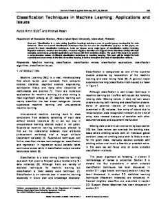
• Example: making credit decisions at American Express UK (cited in [Langley and Simon, 1995])
From [Bose and Mahapatra, 2001]
40
ML Applications
Business
• Example: making credit decisions at American Express UK (cited in [Langley and Simon, 1995]) – Data collection • Questionnaires about people applying for credit
– Initial methodology • Statistical decision process based on discriminant analysis – Reject applicants falling below a certain threshold and accept those above another
• Remaining 10 to 15% of applicants � borderline region � referred to loan officers for a decision. • Loan officers accuracy < 50% – Predicting whether these borderline applicants would default on their loans
41
ML Applications
Business
• Example: making credit decisions at American Express UK (cited in [Langley and Simon, 1995]) – Improved methodology • Input data: 1014 training cases and 18 features (e.g., age and years with an employer, etc.) • Model learning: decision tree using 10 of the 18 features • Evaluation – Accuracy: 70% on the borderline cases – Interpretability: company found the rules attractive because they could be used to explain the reasons for the decisions
42
ML Applications
Business
• Other examples – Find associations between products bought by clients, • E.g., clients who buy science books also buy history books � useful in direct marketing, for example
– Clustering products across client profiles – Detection of fraudulent credit card transactions – Share trading advice –… 43
ML Applications
Entertainment
• Why? – “Intelligent” entertainment products • Automatic music, film or game tagging based on highlevel descriptors (genre, emotion, etc.) • Automatic similarity analysis and recommendation • Advanced playlist generation, based on high-level content, e.g., music emotion • …
44
ML Applications
Entertainment
• How? – Data collection • Necessary to acquire accurate annotation data, which might be difficult due to subjectivity – E.g., music/film tags – Dedicated social networks might be useful (e.g., Last.fm)
– Methodologies • Accuracy is often preferred over interpretability � functional classification algorithms (e.g., SVM) are often useful 45
ML Applications
Entertainment
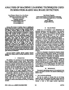
• Example: music emotion recognition and playlist generation [Panda and Paiva, 2011]
46
ML Applications
Entertainment
• Example: music emotion recognition and playlist generation [Panda and Paiva, 2011] – Data collection • Online listening test to annotate songs in terms of arousal and valence
– Feature Extraction • Several relevant audio features(song tempo, tonality, spectral features, etc.)
47
ML Applications
Entertainment
• Example: music emotion recognition and playlist generation [Panda and Paiva, 2011] – Methodologies • Feature selection – RreliefF and Forward Feature Selection
• Regression – Estimation of song arousal and valence based on Support Vector Regression
– Evaluation • R2 statistics: arousal = 63%, valence = 35.6% – Relate to the correlation coefficient(not exactly the square) 48
ML Applications
Entertainment
• Other examples – Classification and segmentation of video clips – Film tagging – Song classification for advertisement, game sound context, music therapy, … – Automatic game playing –…
49
ML Applications
Medicine
• Why? – Support to Diagnosis • Construction of decision-support systems based on medical data to diagnosis support, automatic classification of pathologies, etc.
– Training support • E.g., improve listening proficiency using the stethoscope via detection and classification of heart sounds
50
ML Applications
Medicine
• How? – Data collection • Plenty of physicians’ data in hospitals • In some situations, necessary to acquire data in hospital environment and annotate manually (e.g., echocardiogram data)
– Methodologies • Both accuracy and interpretability are aimed at � rule induction, decision trees and functional classification algorithms (e.g., SVM) are often useful 51
ML Applications
Medicine
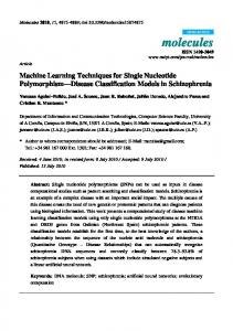
• Example: heart murmur classification [Kumar et al., 2010]
52
ML Applications
Medicine
• Example: heart murmur classification [Kumar et al., 2010] – Data collection • Heart sound were recorded from 15 healthy subjects and from 51 subjects several types of murmurs, from the University Hospital of Coimbra, Portugal. • Acquisition was performed with an electronic stethoscope • Sound samples annotated by a clinical expert
– Feature Extraction • Several relevant audio features (ZCR, transition ratio, spectral features, chaos)
53
ML Applications
Medicine
• Example: heart murmur classification [Kumar et al., 2010] – Methodologies • Classification – 7 classes of heart murmurs, best results with Support Vector Machines
– Evaluation • Sensitivity: 94% – Relates to the test's ability to identify positive results.
• Specificity: 96% – Relates to the test's ability to identify negative results. 54
ML Applications
Medicine
• Other examples – Automatic creation of diagnosis rules – Automatic heart sound segmentation and classification – Treatment prescription – Prediction of recovery rate –…
55
ML Applications
Software Engineering (SE)
• Why? – Simplify software development • “Construction of systems that support classification, prediction, diagnosis, planning, monitoring, requirements engineering, validation, and maintenance”[Menzies, 2002] – E.g., Software quality, size and cost prediction, etc.
56
ML Applications
Software Engineering
• How? – Data collection • Company’s past projects, public benchmarks, etc.
– Methodologies • Many of the practical SE applications of machine learning use decision tree learners [Menzies, 2002] – Knowledge bust be explicit
57
ML Applications
Software Engineering
• Example: predicting software development time at TRW Aerospace (cited in [Menzies, 2002])
From [Menzies, 2002]
58
ML Applications
Software Engineering
• Example: predicting software development time at TRW Aerospace (cited in [Menzies, 2002]) – Developed by Barry W. Boehm, in 1981, when he was TRW’s director of Software Research and Technology – Data collection • COCOMO-I (Constructive Cost Model) database: data from 63 software projects at TRW – Projects ranging in size from 2,000 to 100,000 lines of code, and programming languages ranging from assembly to PL/I. – Projects were based on the waterfall model
59
ML Applications
Software Engineering
• Example: predicting software development time at TRW Aerospace (cited in [Menzies, 2002]) – Feature Extraction • Example of features – Estimated thousand source lines of code (KSLOC), complexity, memory constraints, personnel experience (SE capability, applications experience), … – Of the 40 attributes in the dataset, only six were deemed significant by the learner – Output: software development time (in person months)
– Methodology • CART tree learner 60
ML Applications
Software Engineering
• Other examples – Software quality, size and cost prediction, etc. – Predicting fault-prone modules –…
61
ML Applications
Software Engineering
• Domain specificities – Data starvation • Particularly acute for newer, smaller software companies – Lack the resources to collect and maintain such data
• � Knowledge farming: farm knowledge by growing datasets from domain models [Menzies, 2002] (not discussed in this course) – Use of domain models as a seed to grow data sets using exhaustive or monte carlo simulations. – Then, mine data with machine learning – � Out of the scope of this course 62
ML Applications
Comm. Networks
• Why? – Implementation of “intelligent” network protocols • E.g., intelligent routing mechanisms, network anomaly detection, reliability assessment of communication networks, link quality prediction in wireless sensor networks (WSN), etc.
63
ML Applications
Comm. Networks
• How? – Data collection • Features typically collected at node links • Data often manually or semi-automatically annotated (e.g., link quality)
– Methodologies • Both accuracy and interpretability are aimed at � rule induction, decision trees and functional classification algorithms (e.g., SVM) are often useful
64
ML Applications
Comm. Networks
• Example: MetricMap: link quality estimation in WSN (cited in [Förster and Murphy, 2010])
65
ML Applications
Comm. Networks
• Example: MetricMap: link quality estimation in WSN (cited in [Förster and Murphy, 2010]) – Developed by Wang et al. at Princeton University in 2006 – Data collection • MistLab sensor network testbed • Acquisition of link samples and desired features available at the nodes • Link annotation: good or bad, according to its Link Quality Indication (LQI) value (indicator of the strength and quality of a received packet, introduced in the 802.15.4 standard)
66
ML Applications
Comm. Networks
• Example: MetricMap: link quality estimation in WSN (cited in [Förster and Murphy, 2010]) – Feature Extraction • Locally available information, e.g., RSSI (received signal strength indication) levels of incoming packets, CLA (channel load assessment), etc.
– Methodologies • Classification: decision trees (C4.5), using the WEKA workbench
– Evaluation • Algorithm outperformed standard routing protocols in terms of delivery rate and fairness
67
ML Applications
Comm. Networks
• Other examples – Intelligent routing mechanisms – Network anomaly detection – Reliability assessment of communication networks –…
68
ML Applications
Other Examples
• Computer Security – E.g., Intrusion detection, etc.
• Industrial Process Control – E.g., Intelligent control, i.e., automatic control using machine learning techniques, such as neural networks, rule induction methodologies, etc.
• Fault Diagnosis – In mechanical devices, circuit boards
• Speech Recognition • Autonomous Vehicle Driving • Web Mining – Find the most relevant documents for a search query in a web browser
• … and many, many others… 69
ML Applications
Assignment
• Find a machine learning problem in your field – With input and output data
• Suggested case studies (see datasets.rar) – Software Engineering • Software effort prediction (Desharnais’ dataset and included paper)
– Business • Personal Equity Plan direct marketing decision (see next slides)
– Music Emotion Recognition • Emotion classification/regression in the Thayer plane
– Medicine • Breast cancer recurrence prediction
70
ML Applications
Assignment
• Other case studies – Weka’s examples • Weka’s data folder (/data) • Described in [Witten et al. 2011, chapter 1]
– Software Engineering: • PROMISE(PRedictOr Models In Software Engineering) repositories – https://code.google.com/p/promisedata/
– General • SEASR (Software Environment for the Advancement of Scholarly Research) repository – http://repository.seasr.org/Datasets/UCI/arff/
71
Basic Concepts
Basic Concepts • Concept – What we intend to learn • E.g., when to play golf, based on weather data
• Concept description – Model that results from learning the concept based on data • E.g., decision tree for deciding when to play golf
• Instances – Data samples, individual, independent examples of the concept to be learned • E.g., golf dataset: overcast, 83, 88, false, play
73
Basic Concepts • Features – Attributes that measure different aspects of the instance • E.g., golf dataset: outlook, temperature, humidity, windy
• Labels (or outputs) – Instances’ annotated values, e.g., classes or numeric values • E.g., golf dataset: play / don’t play • Often provided by human experts, who label the instances
74
Basic Concepts • Feature types – Most common • Numeric, continuous • Nominal, i.e., discrete categories
75
Machine Learning Taxonomies • • • •
Paradigms Knowledge Representation Traditions Problem Types
ML Taxonomies • Machine learning algorithms may be categorized according to different taxonomies, e.g. – Learning paradigm: supervised, unsupervised, etc. – Knowledge Representation: black-box, transparentbox – Machine learning tradition: neural networks, genetic algorithms, heuristic search, … – Problem type: classification, regression, clustering, association, etc. –… 77
ML Taxonomies • There is significant overlap among the different taxonomies – E.g., multi-layer perceptrons (MLP) belong to the supervised learning paradigm, neural networks tradition, and can be used for classification and regression – E.g., the k-nearest neighbors algorithms belongs to the case-based paradigm and can be used for classification and regression 78
ML Taxonomies • Each category makes basic assumptions about representation, evaluation and learning algorithms – E.g., multi-layer perceptrons • encode knowledge in terms of connection weights between neurons • in regression problems are evaluated, e.g., based on RMSE or R2 • typical learning algorithm is backpropagation to adjust weights
– E.g., rule induction methods • encode knowledge in terms of explicit interpretable rules • in classification are evaluated, e.g., using precision/recall figures • can be learned via, e.g., decision trees algorithms
79
ML Taxonomies
Learning Paradigms
• Supervised learning – Generates a function that maps inputs to desired outputs. • For example, in a classification problem, the learner approximates a function mapping a vector into classes by looking at input-output examples of the function
– Probably, the most common paradigm – E.g., decision trees, support vector machines, Naïve Bayes, k-Nearest Neighbors, … 80
ML Taxonomies
Learning Paradigms
• Unsupervised learning – Labels are not known during training – E.g., clustering, association learning
• Semi-supervised learning – Combines both labeled and unlabeled examples to generate an appropriate function or classifier – E.g., Transductive Support Vector Machine
81
ML Taxonomies
Learning Paradigms
• Reinforcement learning – It is concerned with how an agent should take actions in an environment so as to maximize some notion of cumulative reward. • Reward given if some evaluation metric improved • Punishment in the reverse case
– E.g., Q-learning, Sarsa
• Instance-based or case-based learning – Represents knowledge in terms of specific cases or experiences – Relies on flexible matching methods to retrieve these cases and apply them to new situations – E.g., k-Nearest Neighbors 82
ML Taxonomies
Knowledge Representation
• Black-box – Learned model internals are practically incomprehensible • E.g., Neural Networks, Support Vector Machines
• Transparent-box – Learned model internals are understandable, interpretable • E.g., explicit rules, decision-trees
83
ML Taxonomies
Traditions
• Different ML traditions propose different approaches inspired by real-world analogies – Neural networks researchers: emphasize analogies to neurobiology – Case-based learning: human memory – Genetic algorithms: evolution – Rule induction: heuristic search – Analytic methods: reasoning in formal logic
• Again, different notation and terminology 84
ML Taxonomies
Problems
• Classification – Learn a way to classify unseen examples, based on a set of labeled examples, e.g., classify songs by emotion categories – E.g., decision trees (e.g., C5.4)
• Regression – Learn a way to predict continuous output values, based on a set of labeled examples, e.g., predict software development effort in person months – Sometimes regarded as numeric classification (outputs are continuous instead of discrete) – E.g., Support Vector Regression
85
ML Taxonomies
Problems
• Association – Find any association among features, not just input-output associations (e.g., in a supermarket, find that clients who buys apples also buys cereals) – E.g., Apriori
• Clustering – Find natural grouping among data – E.g., K-means clustering 86
ML Taxonomies In this course, we categorize machine learning algorithms according to problem types
87
Machine Learning Process
• • •
Data Acquisition Data Pre-Processing Feature Extraction and Processing
• Feature Ranking / Selection/Reduction • Model Learning • Model Evaluation • Model Deployment
ML Process Data Acquisition
Data Pre-Processing
Feature Extraction and Processing
Feature Ranking /Selection/ Reduction
Model Evaluation
Acceptable Results?
Model Learning
yes
Model Deployment
no 89
ML Process
Data Acquisition
• Goals – Get meaningful, representatives examples of each concept to capture, balanced across classes, etc. • E.g., Broad range of patients (age, body mass index, sex, co-morbidities), software (size, complexity, SE paradigms), songs from different styles, …
– Get accurate annotations • E.g., data for module fault error rate, link quality in WSNs, song genre, patient clinical status, etc. 90
ML Process
Data Acquisition
• How? – Careful data acquisition protocol • Representative, diverse and large sample selection (e.g., patients, songs, SE projects) • Definition of measurement protocol – Environment for annotation experiment » E.g., silent room, online test, etc. » E.g., in-hospital data collection such as ECGs, echocardiographies; – Data requirements » E.g., number of channels and sampling frequency in song acquisition 91
ML Process
Data Acquisition
• How? – Careful data annotation protocol • Automatic annotation possible in some cases – E.g., bank data already has desired classes (e.g., payment late or on time)
• Often, manual annotation needed – E.g., music emotion or genre labeling – Can be tedious, subjective and error-prone
92
ML Process
Data Acquisition
• How? – Careful data annotation protocol • Manual annotation process – Use annotation experts » E.g., experts in echocardiography analysis, emotion tagging – Distribute the samples across annotators, guaranteeing that » Each annotator gets a reasonable amount of samples » Each sample is annotated by a sufficient number of people
93
ML Process
Data Acquisition
• How? – Careful data annotation protocol • Manual annotation process – Evaluate sample annotation consistency » Remove samples for which there is not an acceptable level of agreement: e.g., too high standard deviation » � Not good representatives of the concept » In the other cases, keep the average, median, etc. of all annotations
94
ML Process
Data Acquisition
• How? – Careful data annotation protocol • Manual annotation process – Evaluate annotator consistency » Exclude outlier annotators • Annotators that repeatedly disagree with the majority » Perform a test-retest reliability study [Cohen and Swerdlik, 1996] • Select a sub-sample of the annotators to repeat the annotations some time later • Measure the differences between annotations
95
ML Process
Data Acquisition
• Example: Bank data – Plenty of data about clients, product acquisition, services, accounts, investments, credit card data, loans, etc. – � Data acquisition usually straightforward, but • Might be necessary to filter data, e.g., due to noise (see preprocessing later) – E.g., inconsistent client names, birth date, etc.
– Necessary to select diverse data: can be automated • Credit card decision based on past default: some yes and some no (balanced, preferably) • Clients from different regions, incomes, family status, jobs, etc. 96
ML Process
Data Acquisition
• Example: Clinical heart sound data acquisition [Paiva et al., 2012] – Selection of population: as diverse as possible • Healthy and unhealthy, broad range of body mass indexes, both sexes(preferably balanced), broad range of ages, …
97
ML Process
Data Acquisition
• Example: Clinical heart sound data acquisition [Paiva et al., 2012] – Definition of measurement protocol • Conducted by an authorized medical specialist • Patient in supine position, turned left (approximately 45 degrees) – the usual echo observation position for the aortic valve.
• Echo configured for Doppler-mode • Stethoscope positioned in the left sternum border region • Runs of 30-60 sec. data acquisitions of heart sound, echo and ECG repeatedly performed 98
ML Process
Data Acquisition
• Example: Clinical heart sound data acquisition [Paiva et al., 2012] – Data annotation • Annotations of the opening and closing instants of the aortic valve performed by an experienced clinical expert using the echocardiographies
99
ML Process
Data Acquisition
There can be no knowledge discovery on bad data! In some domains, this process is straightforward and can even be automated, but in others it can pose a significant challenge.
100
ML Process
Data Pre-Processing
• Goals – Data preparation prior to analysis • E.g., noise filtering, data cleansing, …
101
ML Process
Data Pre-Processing
• How? – Data conditioning • E.g., signal filtering
– Improve data quality • E.g., data cleaning
102
ML Process
Data Pre-Processing
• Example: Clinical heart sound data acquisition [Paiva et al., 2012] – Synchronize data streams from heart sound, echocardiography and ECG – High-pass filtering to eliminate low frequency noises (e.g., from muscle movements, etc.) – Downsampling to 3 kHz
103
ML Process
Feature Extraction & Processing
• Goals – Extract meaningful, discriminative features • E.g., if musical tempo is important in music emotion recognition, extract it. – But current algorithms for tempo estimation from audio are not 100% accurate…
104
ML Process
Feature Extraction & Processing
• How? – Determine the necessary features • Capable of representing the desired concept • With adequate discriminative capability
– Acquire feature values as rigorously as possible • Some cases are simple and automatic – E.g., bank data, RSSI at a network node
• Others might be complex and need additional tools – E.g., song tempo and tonality estimation, cardiac contractility estimation, … � dedicated algorithms 105
ML Process
Feature Extraction & Processing
• How? – Process features, if needed • • • •
Normalize feature values Discretize feature values Detect and fix/remove outliers …
106
ML Process
Feature Extraction & Processing
• Feature Normalization – Why? • Algorithms such as SVMs or neural networks have numerical problems if features are very different ranges
– How? • Typically, min-max normalization to the [0, 1] interval �����
� − �
= ��� − �
– min / max: minimum / maximum feature value, in the training set – x / xnorm : original / normalized feature value
• [-1, 1] interval also common, e.g., in Multi-Layer Perceptrons
107
ML Process
Feature Extraction & Processing
• Feature Normalization – How? • Other possibilities: z-score normalization �����
�− = �
– µ/σ: feature mean / standard deviation (again, computed using the training set) – Normalized data properties: » Mean = 0 » Standard deviation = 1
108
ML Process
Feature Extraction & Processing
• Feature Discretization – Why? • Some algorithms only work with nominal features, e.g., PRISM rule extraction method
– How? • Equal-width intervals – Uniform intervals: all intervals with the same length
• Equal-frequency intervals – Division such that all intervals have more or less the same number of samples 109
ML Process
Feature Extraction & Processing
• Detection and Fix of Outliers – Why? • Feature values may contain outliers, i.e., values significantly out of range – May be actual values or may indicate problems in feature extraction – Result from measurement errors, typographic errors, deliberate errors when entering data in a database
110
ML Process
Feature Extraction & Processing
• Detection and Fix of Outliers – How? • Detection – Manual/visual inspection of features values, e.g., feature histograms – Automatic outlier detection techniques, e.g., » Define “normal” range: e.g., mean ± 3 std » Mark values outside the range as outliers Probable outliers: measurement errors
111
ML Process
Feature Extraction & Processing
• Detection and Fix of Outliers – How? • Fix – Repeat measurements for detected outliers » New experiment, expert opinion, etc. – Manually correct feature values » E.g., in song tempo, listen to the song and manually substitute the outlier value with the correct tempo) » This can be applied to all detected abnormal cases, not only outliers. But such abnormal cases are usually hard to detect
112
ML Process
Feature Extraction & Processing
• Detection and Fix of Outliers – How? • Remove sample – If no fix is available (e.g., algorithm error in feature estimation) and the dataset is sufficiently large, remove the sample
113
ML Process
Feature Extraction & Processing
• Example: bank data – Features: age, sex, income, savings, products, money transfers, investments – Data cleaning: real world data is • incomplete: e.g., lacking attribute values: marital status = “” • noisy: contains errors or outliers, e.g., Age: -1 • inconsistent: job =“unemployed”, salary = “2000”
– Why? • E.g., past requirements did not demand those data 114
ML Process
Feature Extraction & Processing
• Example: film genre tagging – Audio features, e.g., energy, zcr – Scene transition speed – Number of keyframes –…
115
ML Process
Feature Ranking/Selection/Reduction
• Goals – Remove redundancies � eliminate irrelevant or redundant features • E.g., Bayesian models assume independence between features � redundant features decrease accuracy
– Perform dimensionality reduction • Simpler, faster, more accurate and more interpretable models
116
ML Process
Feature Ranking/Selection/Reduction
• Why? – Improve model performance – Improve interpretability – Reduce computational cost
117
ML Process
Feature Ranking/Selection/Reduction
• How? – Determine the relative importance of the extracted features � feature ranking • E.g., Relief algorithm, input/output correlation, wrapper schemes, etc.
118
ML Process
Feature Ranking/Selection/Reduction
• How? – Select only the relevant features • E.g., add one feature at a time according to the ranking, and select the optimum feature set based on the maximum achieved accuracy (see sections on Model Learning and Evaluation) 80.00% 70.00% Accuracy
60.00%
Optimal number of features
50.00% 40.00% 30.00% 20.00% 10.00% 0.00% 1 15 30 45 70 100 130 143 170 200 300 450 600 Number of features
119
ML Process
Feature Ranking/Selection/Reduction
• How? – Eliminate redundant features • E.g., find correlations among input features and delete the redundant ones
– Map features to a less redundant feature space • E.g., using Principal Component Analysis
120
ML Process
Feature Ranking/Selection/Reduction
• Example: zoo data (automatically classify animals: mammal, bird, reptile, etc.) – Remove features whose merit is under some threshold – Start with milk and successively add features according to the rank (eggs, toothed) and find the optimal model performance (see model learning and evaluation)
average merit 13.672 12.174 11.831 11.552 8.398 7.395 7.004 6.18 5.866 5.502 4.967 4.751 4.478 1.485 0.607 0.132 -0.018
average rank 1 2.175 3.095 3.73 5 6.165 6.915 8.295 9.04 9.875 11.27 11.82 12.62 14.005 14.995 16.19 16.81
attribute milk eggs toothed hair feathers backbone breathes tail airborne fins aquatic catsize legs predator venomous animal domestic
121
ML Process
Model Learning
• Goals – Tackle the respective learning problem by creating a good model from data according to the defined requirements and learning problem • Requirements – Accuracy – Interpretability –…
• Learning problem – Classification, regression, association, clustering
122
ML Process
Model Learning
• Learning Problems – Classification • E.g., decision-tree
– Regression • E.g., linear regression
– Association • E.g., Apriori
– Clustering • E.g., K-means clustering
–… – See Taxonomies: Problems (previous section) – See Algorithms (next chapter), for descriptions of some of the most widely used algorithms 123
ML Process
Model Learning
• How? – Define the training and test sets • Train set: used to learn the model • Test set: used to evaluate the model on unseen data • See section on Model Evaluation
124
ML Process
Model Learning
• How? – Select and compare different models • Performance comparison (see Model Evaluation) – Naïve Bayes is often used as baseline algorithm; C4.5 or SVMs, for example, often perform better (see chapter Algorithms) – Interpretability comparison » E.g., rules are interpretable, SVMs are black-box
It has to be shown empirically from realistic examples that a particular learning technique is necessarily better than the others. When faced with N equivalent techniques, Occam’s razor advises to use the simplest of them.
125
ML Process
Model Learning
• How? – Perform model parameter tuning • • • •
Number of neighbors in k-Nearest Neighbors Kernel type, complexity, epsilon, gamma in SVMs Confidence factor in C4.5 …
126
ML Process
Model Learning
• Example: zoo data – Decision tree (C4.5)
127
ML Process
Model Learning
• Example: zoo data – PART decision list feathers = false AND milk = true: mammal (41.0) feathers = true: bird (20.0) backbone = false AND airborne = false AND predator = true: invertebrate (8.0)
fins = true: fish (13.0) backbone = true AND tail = true: reptile (6.0/1.0) aquatic = true: amphibian (3.0) : invertebrate (2.0)
backbone = false AND legs > 2: insect (8.0) 128
ML Process
Model Learning
• Important Question – What is the effect of the number of training examples, features, number of model parameters, etc., in the learning performance? • Not many definitive answers… • Too many parameters relative to the number of observations � overfitting might happen • Too many features � curse of dimensionality – Convergence of any estimator to the true value is very slow in a high-dimensional space
129
ML Process
Model Evaluation
• Goals – Evaluate model generalization capability in a systematic way • How the model will perform on unseen, realistic, data, – E.g., sometimes test sets are “carefully” chosen (and not in a good way ☺)
– Evaluate how one model compares to another – Show that the learning method leads to better performance than the one achieved without learning • E.g., making credit decisions (see example in the respective chapter) using a decision tree might lead to better results (70%) than the one achieved by humans (50%) 130
ML Process
Model Evaluation
• How? – Use a separate test set • Predict the behavior of the model in unseen data
– Use an adequate evaluation strategy • E.g., stratified 10-fold cross-validation
– Use an adequate evaluation metric • E.g., precision, recall and F-measure
131
ML Process
Model Evaluation
• Common Requirements – Accuracy – Interpretability – There is often a trade-off between accuracy and interpretability • E.g., decision tree: trade-off between succinctness (smaller trees) versus classification accuracy • E.g., rule induction algorithms might lead to weaker results than an SVM
132
ML Process
Model Evaluation
• Why test on unseen data? – Example: learn an unknown linear function y = 3x + 4, with some measurement error • You don’t know the underlying concept, so you acquire some measurements – x in the [0, 10] interval, and the corresponding y values
• Then, you blindly experiment with 2 models – One linear model – Another 10th order polynomial model
133
ML Process
Model Evaluation
• Why test on unseen data? – Example • You measure mean squared error (MSE) and get 0.24 for the linear model and 0.22 for the 10th order polynomial model • You naturally conclude that the polynomial model performs slightly better
134
ML Process
Model Evaluation
• Why test on unseen data? Training set 35 actual linear 10th order poly
30
25
20
15
10
5
0
0
1
2
3
4
5
6
7
8
9
10
135
ML Process
Model Evaluation
• Why test on unseen data? – Example • You then repeat data acquisition using a different range, e.g., x in [10, 20], and compare the observed y with the outputs from the two models • To your surprise, you observe a 0.19 MSE for the linear model and a 1.07E+12 MSE for the polynomial model!!! • That’s overfitting: your polynomial model was overly adjusted to the training data
136
ML Process
Model Evaluation
• Why test on unseen data? New data 60 actual linear 10th order poly
55
50
45
40
35
30 10
11
12
13
14
15
16
17
18
19
20
137
ML Process
Model Evaluation
• Why test on unseen data? – Answer: minimize overfitting • Overfitting occurs when the model is overly adjusted to the data employed in its creation, and so the model “learns beyond the concept”, e.g., learns noise or some other concept, but not the underlying concept
– Answer: have a realistic estimate of model performance in unseen data A more accurate representation in the training set is not necessarily a more accurate representation of the underlying concept! 138
ML Process
Model Evaluation
• Basic Definitions – Training set • Set of examples used to learn the model, i.e., to train the classifier, regressor, etc.
– Test set • Independent, unseen, examples used to evaluate the learnt model
139
ML Process
Model Evaluation
The test set must not be used in any way to create the model! Beware of feature normalization, feature selection, parameter optimization, etc.
The larger the training set, the better the classifier! Diminishing returns after a certain volume is exceeded.
The larger the test set, the better the accuracy estimate!
140
ML Process
Model Evaluation
• Basic Definitions – Bias-Variance Dilemma • Bias – Difference between this estimator's expected value and the true value » E.g., we are trying to estimate model performance using a limited dataset and we want the estimated performance to be as close as possible to the real performance » Unbiased estimator: zero bias
• Variance – Variability of estimator: we also want it to be as low as possible
• In practice, there is often a trade-off between minimizing bias and variance simultaneously 141
ML Process
Model Evaluation
• Basic Definitions – Bias-Variance Dilemma
From http://scott.fortmann-roe.com/docs/BiasVariance.html
142
ML Process
Model Evaluation
• Evaluation Strategies (see [Refaeilzadeh et al. 2009]) – Training set (a.k.a Resubstitution Validation) • Idea – Evaluate model performance using some metric (see section Evaluation Metrics) resorting only to the training set » I.e., train using the entire dataset, evaluate using the same entire dataset (i.e., validate with resubstitution)
143
ML Process
Model Evaluation
• Evaluation Strategies – Training set (a.k.a Resubstitution Validation) • Limitations – Accuracy on the training set overly optimistic � not a good indicator of the performance on the test set – Overfitting often turns out – � High bias
• Advantages – Have an idea of data quality » Low training accuracy in the training set may indicate poor data quality, missing relevant features, dirty data, etc. 144
ML Process
Model Evaluation
• Evaluation Strategies – Hold-out • Idea – Separate the entire set into two non-overlapping sets » Training set: typically, 2/3 • Rule of thumb: training set should be more than 50% » Test set: unseen data, typically 1/3 (data held out for testing purposes and not used at all during training) – Learn (train) the model in the first set – Evaluate in the second set
145
ML Process
Model Evaluation
• Evaluation Strategies – Hold-out • Limitations – Results highly dependent on the train/test split » Training/test sets might not be representative • In the limit, the training set might contain no samples of a given class… • The cases in the test set might be too easy or too hard to classify – Again, high bias and high variance
146
ML Process
Model Evaluation
• Evaluation Strategies – Hold-out • Limitations – Requires a large dataset, so that the test set is sufficiently representative » Often unavailable… • Manual annotation typically requires specialized human expertise and takes time � datasets are often small
147
ML Process
Model Evaluation
• Evaluation Strategies – Stratified Hold-out • Idea – In classification, hold-out with classes balanced across the training and test set (i.e., stratification) » Promotes sample representativity in the two sets, due to class balancing
• Advantages – May reduce bias, due to higher representativity, but it is not as low as could be, e.
• Limitations – High variance still unsolved – Still requires a large dataset 148
ML Process
Model Evaluation
• Evaluation Strategies – Repeated (Stratified) Hold-out • Idea – Repeat the training and testing process several times with different random samples and average the results » Typically, between 10 and 20 repetitions
• Advantages – Lower variance observed in performance estimation due to repetition
149
ML Process
Model Evaluation
• Evaluation Strategies – Repeated (Stratified) Hold-out • Limitations – Bias could be lower » Typically, some data may be included in the test set multiple times while others are not included at all » Some data may always fall in the test set and never contribute to the learning phase
150
ML Process
Model Evaluation
• Evaluation Strategies – (Repeated) (Stratified) Train-Validate-Test (TVT) • Idea – 3 independent datasets – Training set: learn the model – Validation set: used to evaluate parameter optimization, feature selection, compare models, etc. – Test set: used to evaluate the final accuracy of the optimized model
151
ML Process
Model Evaluation
• Evaluation Strategies – (Repeated) (Stratified) Train-Validate-Test (TVT) • Limitations – Again, requires an even larger dataset, so that test and validation sets are sufficiently representative – Same bias and variance limitations
152
ML Process
Model Evaluation
• Evaluation Strategies – Repeated Stratified K-fold Cross-Validation • Idea 1. 2. 3. 4.
5.
Randomly separate the entire set into a number of stratified k equal-size folds (partitions) Train using k-1folds, test using the remaining fold Repeat training and testing (step 2) k times, alternating each fold in the test set Repeat steps 1 to 3 a number of times (reshuffle and restratify data) » Typically, 10 to 20 times Average the results
153
ML Process
Model Evaluation
• Evaluation Strategies – Repeated Stratified K-fold Cross-Validation
Illustration of 3-fold cross validation [Refaeilzadeh et al. 2009]
154
ML Process
Model Evaluation
• Evaluation Strategies – Repeated Stratified K-fold Cross-Validation • Recommended k – High k: lower bias, higher variance – Low k: higher bias, lower variance – Typically, k = 10, i.e., 10-fold cross validation » Mostly, empirical result » Good bias-variance trade-off
Method of choice in most practical situations!
155
ML Process
Model Evaluation
• Evaluation Strategies – Repeated Stratified K-fold Cross-Validation • Advantages – Guarantees that all samples appear in the test set � lower bias » Average repeated, stratified, 10-fold cross-validated performance considered a good estimate of model performance on unseen data – Lower variance » Repetition of the experiment shows low performance variance – Good bias-variance trade-off – Useful for performance prediction based on limited data 156
ML Process
Model Evaluation
• Evaluation Strategies – Repeated Stratified K-fold Cross-Validation • Limitations – Computational cost » 10 x 10-folds is expensive for large and complex datasets, or complex model learning algorithms • � 5-fold might be used in such cases
157
ML Process
Model Evaluation
• Evaluation Strategies – Nested RS K-fold Cross-Validation • Idea – Nest repeated (R) stratified (S) K-fold cross-validation (CV) if model structure or parameter tuning is a goal » E.g., tune SVM parameters, perform feature selection, find out how many hidden layer neurons in an MLP
• Test set should never be used during training! – � use an outer CV for testing and an inner CV for structure/parameter learning » Conceptually similar to the train-validate-test strategy, but without bias and variance limitations
158
ML Process
Model Evaluation
• Evaluation Strategies – Leave-One-Out Cross-validation • Idea – Cross- validation (CV) where each fold contains only one sample, i.e., n-fold CV (n = number of samples)
• Advantages – Deterministic: no random selection involved � no need for repetition – Low bias – Greatest possible amount of data for training � increases the chance that the classifier is a good one – Adequate for particularly small datasets
159
ML Process
Model Evaluation
• Evaluation Strategies – Leave-One-Out Cross-validation • Limitations – High variance – Non-stratified test set » A model based on the majority class will always make a wrong prediction in a 2-class problem… – Computational time » Might be infeasible in very large datasets
160
ML Process
Model Evaluation
• Evaluation Strategies – (Repeated) Bootstrap • Idea – Based on the procedure of sampling with replacement, i.e., select the same sample more than once – Training set: get the original dataset and sample with replacement » This set will typically contain 63.2% of all samples (so, the method is often termed 0.632 bootstrap – Test set: unselected samples (36.8%) – Error estimation: use the two sets » e = 0.632 × etest instances + 0.368 × etraining instances
161
ML Process
Model Evaluation
• Evaluation Strategies – (Repeated) Bootstrap • Advantages – Probably the best way for accuracy estimation in very small datasets
– Expert examination • Might be necessary, e.g., in unsupervised learning
162
ML Process
Model Evaluation
• Performance Metrics – Classification • Precision/Recall, F-measure, error rate
– Regression • Root mean squared error, correlation, R2 statistics
– Clustering • If labels are available, compare created clusters with class labels; otherwise, expert evaluation
– Association • Expert evaluation 163
ML Process
Model Evaluation
• Performance Metrics – Classification problems Sample nr.
Real class
Predicted class
1
M
M
2
M
M
3
M
B
4
M
M
5
M
M
6
M
R
7
M
M
8
B
B
9
B
B
10
B
R
11
B
B
12
B
B
13
R
R
14
R
R
15
R
M
16
R
B
17
R
R
Example: Animal classification: mammal (M), bird (B) or reptile (R) Test set: Mammal: 7 samples (2 errors) Bird: 5 samples (1 error) Reptile: 5 samples (2 errors)
164
ML Process
Model Evaluation
• Performance Metrics – Classification problems • Confusion matrix (or contingency table) – Matrix distribution of classifications through classes » Lines: distribution of real samples » Columns: distribution of predictions – Goal: zeros outside the diagonal – Example: animals M
B
R
M
5
1
1
B R
0 1
4 1
1 3
Predicted as M
Actual
Actual
Predicted as M B R
B
R
71.43% 14.23% 14.23% 0% 20%
80% 20%
20% 60%
165
ML Process
Model Evaluation
• Performance Metrics – Classification problems • Confusion matrix (CM) or contingency table – Some properties » Sum across line: number of actual samples of the class in that line • E.g., line M: 5 + 1 + 1 = 7 actual mammals » Sum across column: number of predictions that fall in that class • E.g., column M: 5 + 0 + 1 = 6 samples predicted as mammals – Confusion matrix more useful when percentages shown » E.g., line M: 5/7, 1/7, 1/7 = 71.43%, 14.23%, 14.23%
166
ML Process
Model Evaluation
• Performance Metrics – Classification problems • Error rate – Proportion of errors made over the test set #��� � ����� � ��� � � ����� ���� = �
» # = “number of” » N: total number of test samples – Goal: minimize error rate – Example: animals » 5 errors in 17 cases � 5/17 = 29.4% error rate • # errors = sum of non-diagonal values in the CM 167
ML Process
Model Evaluation
• Performance Metrics – Classification problems • Accuracy (or success rate) – Proportion of correct classifications over the test set �������� = 1 − ����� ���� =
#������� ����� � ��� � � �
– Goal: maximize accuracy – Example: animals » 12 correct classifications in 17 cases � 12/17 = 70.59% accuracy • # correct = sum of diagonal values in the CM 168
ML Process
Model Evaluation
• Performance Metrics – Classification problems • Class True Positive (TP) rate – True positives: samples predicted to belong to class i that actually belong to that class, i.e., class accuracy �� ���� =
�� �
» TPi: number of true positives of class I » Ni: number of samples that belong to class i – Goal: maximize TP rate 169
ML Process
Model Evaluation
• Performance Metrics – Classification problems • Class True Positive (TP) rate – TPi: diagonal value of the confusion matrix – Ni: sum of line i Predicted as Actual
M M B R
B
R
TPM TPB TPR
170
ML Process
Model Evaluation
• Performance Metrics – Classification problems • Class True Positive (TP) rate – Example: animals » Class M: TPM = 5; NM = 7 � TP rateM = 71.43% » Class B: TPB = 4; NB = 5 � TP rateB = 80% » Class R: TPR = 3; NR = 5 � TP rateR = 60%
171
ML Process
Model Evaluation
• Performance Metrics – Classification problems • Global True Positive (TP) rate – Weighted average of TP rates for individual classes �� ���� =
#
1 ! � ∙ �� ���� �
%$» C: number of classes – The same as accuracy – Animals example » TP rate = 1/17 x (7 x 71.43 + 5 x 80 + 5 x 60) = 70.59% 172
ML Process
Model Evaluation
• Performance Metrics – Classification problems • Class False Positive (FP) rate – False positives: samples that do not belong to class i but that are predicted as that class &� ���� =
&� �
» FPi: number of false positives of class I » � : number of samples that do not belong to class I – Goal: minimize FP rate 173
ML Process
Model Evaluation
• Performance Metrics – Classification problems • Class True Positive (TP) rate – FPi: sum of column i cells of, excerpt for the diagonal – � : sum of all lines, except for i
Actual
Predicted as M
B
R
M
TPM
FPB
FPR
B R
FPM FPM
TPB FPB
FPR TPR
174
ML Process
Model Evaluation
• Performance Metrics – Classification problems • Class False Positive (FP) rate – Animals example » Class M: FPM = 1 (sample 15); �' = 5 + 5 = 10 (5 B + 5 R) � FP rateM = 10% » Class B: FPB = 2; �( = 7 + 5 = 12 � FP rateB = 16.67% » Class R: FPR = 2; �) = 7 + 5 =12 � FP rateR = 16.67%
175
ML Process
Model Evaluation
• Performance Metrics – Classification problems • Global False Positive (FP) rate – Weighted average of FP rates for individual classes &� ���� =
1
∑#$% �
#
! � ∙ &� ����
%$– Animals example » FP rate = 1/34 x (10 x 10 + 12 x 16.67 + 12 x 16.67) = 14.71%
176
ML Process
Model Evaluation
• Performance Metrics – Classification problems • Class Precision – Fraction of samples predicted as class i that indeed belong to class i – Related to the incidence of false alarms +��� � � =
�� �� , &�
– Denominator: sum of column i
Attention! In this context, precision is very different than accuracy!!! 177
ML Process
Model Evaluation
• Performance Metrics – Classification problems • Class Precision – Animals example » Class M: precisionM = 5 / (5 + 1) = 83.33% » Class B: precisionB = 4 / (4 + 2) = 66.67% » Class R: precisionR = 3 / (3 + 2) = 60%
178
ML Process
Model Evaluation
• Performance Metrics – Classification problems • Global Precision – Weighted average of precision for individual classes +��� � � =
#
1 ! � ∙ +��� � �
�
%$– Animals example » precision = 1/17 x (7 x 83.33 + 5 x 66.67 + 5 x 60) = 71.57%
179
ML Process
Model Evaluation
• Performance Metrics – Classification problems • Class Recall – Fraction of samples of class i that are correctly classified » i.e., accuracy of class i, the same as TP ratei �� ������ = �� , &�
» FNi: number of false negatives of class I • Elements of class I that are incorrectly classified, i.e., falsely classified as not belong to that class (hence, false negatives) – Denominator: sum of line i 180
ML Process
Model Evaluation
• Performance Metrics – Classification problems • Class Recall CM focused on columns (precision)
CM focused on lines (recall) Predicted as
M
B
R
M
TPM
FPB
FPR
B R
FPM FPM
TPB FPB
FPR TPR
Actual
Actual
Predicted as
M
B
R
M
TPM
FNM
FNM
B R
FNB FNR
TPB FNR
FNB TPR
181
ML Process
Model Evaluation
• Performance Metrics – Classification problems • Class Recall – Animals example » Class M: recallM = 5 / (5 + 2) = 71.43% » Class B: precisionB = 4 / (4 + 1) = 80% » Class R: precisionR = 3 / (3 + 2) = 60%
182
ML Process
Model Evaluation
• Performance Metrics – Classification problems • Global Recall – Weighted average of recall for individual classes » = accuracy = TP rate ������ =
#
1 ! � ∙ ������ �
%$– Animals example » recall = 1/17 x (7 x 71.43 + 5 x 80 + 5 x 60) = 70.59%
183
ML Process
Model Evaluation
• Performance Metrics – Classification problems • Class F-measure – F-measure: a.k.a. F-score or F1-score or balanced F1-score – Combination of precision (related to the incidence of false alarms) and recall (class accuracy) into a single metric » Harmonic mean of precision (P) and recall (R) & − ������� = 2
� ∙. � ,.
184
ML Process
Model Evaluation
• Performance Metrics – Classification problems • Class F-measure – Animals example » Class M: F-measureM = 76.92% » Class B: F-measureB = 72.72% » Class R: F-measureR = = 60%
185
ML Process
Model Evaluation
• Performance Metrics – Classification problems • Global F-measure – Weighted average of F-measure for individual classes &−������� =
#
1 ! � ∙ &−������� �
%$– Animals example » F-measure = 1/17 x (7 x 76.92 + 5 x 72.72 + 5 x 60) = 70.71%
186
ML Process
Model Evaluation
• Performance Metrics – Classification problems • Most common metrics – Precision, recall, F-measure – Sensitivity and specificity (often used in medicine) » Sensitivity = recall = TP rate » Specificity = 1 – FP rate • Proportion of people with a disease with a negative test
• Other metrics
187
ML Process
Model Evaluation
• Performance Metrics – Classification problems • Other metrics [Witten et al., 2011, pp. 166-178] – – – – – –
Cost-Benefit Analysis Lift Charts ROC (Receiver Operating Characteristic) curves AUC: Area Under the ROC Curve Precision-recall curves Cost curves
188
ML Process
Model Evaluation
• Performance Metrics – Classification problems • Other metrics
http://csb.stanford.edu/class/public/lectures/lec4/Lecture6/Data_Visualization/pages/Roc_Curve_Examples.html
ML Process
Model Evaluation
• Performance Metrics – Classification problems • Learning class probabilities – Instead of black and white classification (belongs or doesn’t belong to class), learn the probability of belonging to each class – E.g., Naïve Bayes, SVMs can output class probabilities – Metrics [Witten et al., 2011, pp. 159-163] » Quadratic Loss Function » Informational Loss Function
190
ML Process
Model Evaluation
• Performance Metrics – Regression problems Sample nr.
Real Temp
Predicted Temp
1
27.2
23.4
2
31.4
27.2
3
12.3
15.4
4
2.4
0.1
5
-3.8
0.2
6
7.2
5.3
7
29.7
25.4
8
34.2
33.2
9
15.6
15.6
10
12.3
10.1
11
-5.2
-7.2
12
-10.8
-8.1
13
14.2
15.3
14
41.2
38.4
15
37.6
34.5
16
19.2
17.8
17
8.3
8.5
Example: Predict temperature for next day at 12:00pm: 50 40 30 20
real
10
predicted
0 1 2 3 4 5 6 7 8 9 10 11 12 13 14 15 16 17 -10 -20
191
ML Process
Model Evaluation
• Performance Metrics – Regression problems • RMSE – Root (R) mean (M) squared (S) error (E): metric of average sample error ./01 =
3
1 ∙ ! � − �+ �
%$2
./01 = /01 1 /01 = ∙ 001 �
3
001 = ! � − �+
2
%$» yi: actual value of sample i » ypi: value predicted for sample i – Goal: minimize RMSE 192
ML Process
Model Evaluation
• Performance Metrics – Regression problems • RMSE – Temperature example » SSE = 479.54 » MSE = 28.21 » RMSE = 5.31 degrees
193
ML Process
Model Evaluation
• Performance Metrics – Regression problems • Pearson’s Correlation Coefficient (R) – Measure of the linear correlation between two variables ∑3$% � − �4 ∙ �+ − �+ . �, �+ = 3 ∑ $% � − �4 2 ∙ ∑3$% �+ − �+
2
» �4: mean of actual values » �+: mean of actual values – Range: [-1, 1] » 1: perfect correlation, -1: perfect inverse correlation, 0: no correlation – Goal: maximize R 194
ML Process
Model Evaluation
• Performance Metrics – Regression problems • Pearson’s Correlation Coefficient (R) – Temperature example » R = 94.4%
195
ML Process
Model Evaluation
• Performance Metrics – Regression problems • Coefficient of Determination (R2) – Several different definitions » E.g., square of correlation coefficient » Most common 001 . =1− 00� 2
3
00� = ! � − �4
2
%$• SST: total sum of squares: (proportional to the sample variance) • Range: ]-inf, 1] Goal: maximize R2 196
ML Process
Model Evaluation
• Performance Metrics – Regression problems • Coefficient of Determination (R2) – Temperature example » �4: 16.06 » SSE = 479.54 » SST = 3905.5 » R2 = 87.72%
197
ML Process
Model Evaluation
• Performance Metrics – Regression problems • Other metrics [Witten et al., 2011, pp. 166-178] – – – –
Mean Absolute Error Relative Absolute Error Relative Squared Error Root Relative Squared Error
198
ML Process
Model Evaluation
• Comparison of Different Models – Statistical tests • Guarantee that the observed differences are not caused by chance effects • Methods [Witten et al., 2011, pp. 166-178] – Student’s T-test – Paired T-test
199
ML Process
Model Evaluation
• Are results acceptable? – What are acceptable results? • Perfect results – 100% accuracy ☺
• Results that outperform the state-of-the-art – Accuracy, generalization capability, decision speed, etc. – E.g., human credit decisions, diagnosis, etc.
200
ML Process
Model Evaluation
• Are results acceptable? – Yes � Deploy system (see next section)
201
ML Process
Model Evaluation
• Are results acceptable? – No � Go back and repeat the necessary steps: find out causes and attempt to fix… • Missing features? – Critical features to the concept bay be missing, e.g., articulation is difficult to extract from audio but is important to model emotion � devise methods to obtain the missing features
• Redundant features still present? – Repeat feature selection with different algorithms, use domain knowledge about important features, etc. 202
ML Process
Model Evaluation
• Are results acceptable? – No � Go back and repeat the necessary steps: find out causes and attempt to fix… • Error in measurements too high? – E.g., tempo estimation in audio can be error-prone � improve measurement methods, manually correct measurements, …
• Bad annotations? – Output values badly assigned (subjective concept, annotations by non-experts, etc.) � repeat annotation experiment
203
ML Process
Model Evaluation
• Are results acceptable? – No � Go back and repeat the necessary steps: find out causes and attempt to fix… • Data acquisition poorly conducted? – Samples might not be representative of the concept, many outliers, narrow range of samples, … � repeat data acquisition
• Inadequate model? – E.g., linear model to fit to non-linear data � experiment with different models
• … 204
ML Process
Model Deployment
• Goals – Put the learned model into real-world production – Support actual decision-making
Machine learning tools should be used for decisionsupport, not decision-making. Human experts must have the final word, especially in critical cases (e.g., health)!
205
ML Process
Model Deployment
• How? – Simple written set of rules for decision-making – Complex piece of software • Automatic classification, prediction, clustering, association rules, etc. for new, real-world data
– Validation by human expert typically necessary • Models are imperfect � human validation often necessary, especially for critical tasks – E.g., medical diagnosis
• � Usually, models are not completely autonomous, instead, support decision-making by a human
206
ML Process
Model Deployment
• Final Model – Use the entire dataset to learn the final model • With the selected features • With the optimal parameters determined • Expected performance – The average cross-validation performance
207
Algorithms
• • •
Classification Regression Clustering
• Association • Feature Ranking/Selection • Dimensionality Reduction
Algorithms • General Remarks – Know your data • Is there a single/short number of attributes that discriminates your classes? • Are features independent or you can find any strong correlations among them? • Are attributes linearly or non-linearly dependent? • Is there any missing data? Do you need a method capable of dealing with this? • Mix of nominal and numerical attributes? Do you a need a method that can handle both? Or should you convert numeric data to nominal or vice-versa? 209
Algorithms • General Remarks – Know your goals • • • •
Find associations between features? Find natural groupings in data? Classify your data? Single-class or multi-class problem? Numerical outputs? Or should you discretize the outputs? • Do you need to extract explicit knowledge in form of rules? Are decision trees sufficient for that purpose? Or do you need a more compact representation? 210
Algorithms • General Remarks – Occam’s Razor • � simplicity-first methodology – Only if a simple algorithm doesn’t do the job, try a more complex one
– No magical recipes • There’s no single algorithm that suits all problems!
211
Algorithms • Categories of algorithms – Learning problem: classification, regression, … – Complexity: basic, advanced – Algorithm type • Probabilistic: algorithms based on probability theory • Functional: representation is a mathematical function, e.g., linear regression, SVM • Lazy: no explicit model training is carried out, e.g., KNN • Trees: representation is a decision tree, e.g., ID3, C4.5 212
Algorithms • Categories of algorithms – Algorithm type: • Rule-induction: knowledge represented as explicit rules, e.g., PRISM • Clustering: e.g., k-means clustering, ExpectationMaximization • Association rules: e.g., APRIORI • Feature ranking/selection: e.g., Relief, forward feature selection, correlation-based ranking • Dimensionality reduction: e.g., Principal Component Analysis 213
Algorithms • Algorithm details – See [Mitchell, 1997; Witten et al. 2011]
214
Algorithms
Classification - Basic
• Decision Trees – C4.5 is an international standard in machine learning; – most new machine learners are benchmarked against this program. – C4.5 uses a heuristic entropy measure of information content to build its trees – C4.5 runs faster for discrete attributes • performance on continuous variables tend to be better 215
Algorithms
Classification
• Decision Trees – C4.5 is an international standard in machine learning; – most new machine learners are benchmarked against this program. – C4.5 uses a heuristic entropy measure of information content to build its trees – C4.5 runs faster for discrete attributes • performance on continuous variables tend to be better 216
Algorithms
Classification
• Decision Trees – Drawback with decision tree learners is that they can generate incomprehensibly large trees – In C4.5, the size of the learnt tree is controlled by the minobs command-line parameter. – Increasing minobs produces smaller and more easily understood trees – However, increasing minobs also decreases the classification accuracy of the tree since infrequent special cases are ignored 217
Algorithms
Classification
• Decision Trees – execute very quickly and are widely used
218
Algorithms
Classification
• Decision Trees
219
Algorithms
Classification
• Rule Induction – Rules illustrate the potential role of prior knowledge (domain knowledge) • There are methods focused on the integration of such domain knowledge in the learning process
220
Algorithms
Regression
• About regression – Regression equation • y = f(f1, f2, …, fn; P)
– Regression • Process of determining the weights
– Goal • Optimize parameters P that maximize prediction accuracy, measure according to the previous metrics (e.g., minimize RMSE, maximize R2, …)
221
Algorithms
Regression
• Linear Regression – Regression equation: linear equation • Y = a1f1 + a2f2 + a3f3 + … + anfn
– Limitations • Incapable of discovering non-linear relationships
222
Algorithms
Association
• About Association Learning (p. 41) – Differ from classification learning in two ways • Can predict any attribute, not just the class • Can predict more then one attribute at a time
223
Algorithms
Association
• About Association Learning The “diapers and beer” story: article in London’s Financial Times (February 7, 1996) “The oft-quoted example of what data mining can achieve is the case of a large US supermarket chain which discovered a strong association for many customers between a brand of babies’ nappies (diapers) and a brand of beer. Most customers who bought the nappies also bought the beer. The best hypothesisers in the world would find it difficult to propose this combination but data mining showed it existed, and the retail outlet was able to exploit it by moving the products closer together on the shelves.” This is part fact, part myth: “In reality they never did anything with beer and diapers relationships. But what they did do was to conservatively begin the reinvention of their merchandising processes (see http://www.dssresources.com/newsletters/66.php).
224
Advanced Topics
Advanced Topics
Ensemble Learning
• Ensemble Learning: bagging, boosting, stacking – Idea: combine the output of several different models � make decisions more reliable
226
Advanced Topics
Ensemble Learning
• Multi-class Learning Schemes – One-against-All – One-against-One
• Multi-label Classification – Multi-label instances (p. 40) • E.g., songs are often annotated with several emotion tags, not just one � multi-label classification problem, not addressed here
227
Algorithms
Classification
• About Classification Learning
228
Advanced Topics
Ensemble Learning
• •
1) Regras de classificação/previsão - Se feature A baixa e feature B alta então valência média...
• •
2) Association analysis: - e.g., músicas que pertencem à classe 1 também pertencem à classe 5? (complementa ponto 3) - All Music: músicas com várias labels de classes diferentes, e.g. 1 e 5? - Associação de features: músicas com a feature A na gama A têm a feature B na gama B - Regras de associação entre features (todas: input e output)
• • •
•
3) Clustering automático (isto não é extracção de conhecimento, é classificação, mais ou menos): - tentar fazer clustering não-supervisionado com 5 classes ou tentar encontrar o número automaticamente - Detectar sobreposições entre classes
• • •
4) Detecção de outliers: - para cada classe, analisar features individualmente (ou em grupo...) e procurar outliers - repetir classificação sem outliers?
• •
229
Advanced Topics
Ensemble Learning
• 5) Class description: • - que features são relevantes para cada classe? Entre em jogo a versão 1 vs all com features diferentes para cada classe • - Analisar dispersão das features em cada classe • 6) Class discrimination: • - que features distinguem classes? • - culminar num classificador hierárquico 230
Conclusions and Future Work
Conclusions and Future Work • Conclusions – This document summarized some of main issues involved in the machine learning process
• Future Work – Algorithms – Advanced algorithms and techniques
232
Acknowledgements
Acknowledgements Proyecto Prometeo, Ecuador
Escuela Politécnica Nacional, Quito, Ecuador Universidade de Coimbra, Portugal 234
About the Author
About the Author • More info at http://rppaiva.dei.uc.pt/
236
References
References • Main Mitchell T. M. (1997). Machine Learning, McGraw-Hill Science/Engineering/Math. Witten I. H., Frank E. and Hall M. A. (2011). Data Mining: Practical Machine Learning Tools and Techniques (3 ed.), Elsevier.
238
References • Additional Bose I. and Mahapatra R. K. (2001). “Business data mining — a machine learning perspective”, Information & Management, Vol. 39(3), pp. 211-225. Cohen R. J. and Swerdlik M. (1996). Psychological Testing and Measurement: An Introduction to Tests and Measurement, Mountain View, CA, Mayfield Publishing Company. Förster A. and Murphy A. L. (2010). “Machine Learning Across the WSN Layers”, in Wireless Sensor Networks, Förster A. and Förster A. (Eds.), InTechWeb Publishing Kumar et al. (2010). “Heart Murmur Classification using Complexity Signatures”, 20th International Conference on Pattern Recognition.
239
References • Additional Langley P. and Simon H. A. (1995). “Applications of Machine Learning and Rule Induction”, Communications of the ACM, Vol. 38, pp. 55-64. Menzies T. (2002). “Practical Machine Learning for Software Engineering and Knowledge Engineering”, in Handbook of Software Engineering and Knowledge Engineering - Volume I: Fundamentals, Chang S. K. (Ed.), World Scientific Pub. Paiva R. P., Carvalho P., Couceiro R., Henriques J., Antunes M., Quintal I. & Muehlsteff J. (2012). “Beat-to-Beat Systolic Time-Interval Measurement from Heart Sounds and ECG”. Physiological Measurement , Vol. 33, pp. 177194, IOP Science. Panda R. and Paiva R. P. (2011). “Automatic Creation of Mood Playlists in the Thayer Plane: a Methodology and a Comparative Study”. 8th Sound and Music Computing Conference – SMC’2011, Padova, Italy
240
References • Additional Refaeilzadeh P., Tang L. and Liu H. (2009). “CrossValidation”, Encyclopedia of Database Systems, Ling L. and M. Tamer (Eds.), pp. 532-538 Svensson M. and Söderberg J. (2008). “Machinelearning technologies in telecommunications”, Ericsson Review 2008(3), pp. 29-33 Zhang D. and Tsai J. J. P. (2005). Machine Learning Applications in Software Engineering, World Scientific Publishing. 241