Session 4D: Graph Mining 1
CIKM’17, November 6-10, 2017, Singapore
MGAE: Marginalized Graph Autoencoder for Graph Clustering Chun Wang
Centre for Artificial Intelligence University of Technology Sydney Sydney, NSW 2007, Australia
[email protected]
Shirui Pan∗
Centre for Artificial Intelligence University of Technology Sydney Sydney, NSW 2007, Australia
[email protected]
Xingquan Zhu
Guodong Long
Centre for Artificial Intelligence University of Technology Sydney Sydney, NSW 2007, Australia
[email protected]
Jing Jiang
Dept. of CEECS Florida Atlantic University Boca Raton, FL 33431, USA
[email protected]
Centre for Artificial Intelligence University of Technology Sydney Sydney, NSW 2007, Australia
[email protected]
ABSTRACT
1
Graph clustering aims to discover community structures in networks, the task being fundamentally challenging mainly because the topology structure and the content of the graphs are difficult to represent for clustering analysis. Recently, graph clustering has moved from traditional shallow methods to deep learning approaches, thanks to the unique feature representation learning capability of deep learning. However, existing deep approaches for graph clustering can only exploit the structure information, while ignoring the content information associated with the nodes in a graph. In this paper, we propose a novel marginalized graph autoencoder (MGAE) algorithm for graph clustering. The key innovation of MGAE is that it advances the autoencoder to the graph domain, so graph representation learning can be carried out not only in a purely unsupervised setting by leveraging structure and content information, it can also be stacked in a deep fashion to learn effective representation. From a technical viewpoint, we propose a marginalized graph convolutional network to corrupt network node content, allowing node content to interact with network features, and marginalizes the corrupted features in a graph autoencoder context to learn graph feature representations. The learned features are fed into the spectral clustering algorithm for graph clustering. Experimental results on benchmark datasets demonstrate the superior performance of MGAE, compared to numerous baselines.
Network applications, such as social networks, citation networks, and protein interaction networks, have emerged increasingly and have attracted much attention in the last decade. Unlike traditional data which are represented as a flat-table or vector format, networked data are naturally represented as graphs for characterizing the individual properties of each node and capturing the pairwise structure relationship between nodes in the networks. The complexity of networked data has imposed many challenges on machine learning tasks, such as graph clustering. Given a graph (network) with node content and structure (link) information, graph clustering aims to partition the nodes in the graph into a number of disjoint groups. This has become one of the most important tasks in many applications, such as community detection [6], customer group segmentation [14], and functional group discovery in enterprise social networks [12]. The major challenge of graph clustering is how to effectively utilize the information in the graph. Shallow Representation for Graph Clustering: To enable graph clustering, a vast number of algorithms and theories have been developed, most of which can be considered as shallow methods that directly perform clustering or learn simple or linear representations from the given graph. Early clustering methods on graphs mainly focus on graph structure only. They either capture the betweenness of edges [7], compute eigenvectors of the graph Laplacian [20, 21], or employ belief propagation [10] to exploit the graph structure. Recently, overlapping community detection algorithms, like BigClam [39] and AgmFit [38], have also been developed; however, these algorithms are suboptimal because they only use one channel of information and ignore the other. When considering integrating both node content and network information, early methods in [1, 8] apply a nonnegative matrix factorization (NMF) strategy to decompose node content matrix and use graph structure as regularization terms. Relational topic model methods [3, 29] try to simultaneously model both the links and the contents for clustering. Zhou et al. add virtual attribute nodes and edges in a network and compute the similarity based on the augmented network [41]. By considering a graph as a dynamic system and modeling its structure as a consequence of interactions among nodes, Liu et al. proposed an algorithm from the view of content propagation and then modeled the interactions with
KEYWORDS Graph clustering; autoencoder; graph autoencoder; graph convolutional network; network representation.
∗ Corresponding
INTRODUCTION
Author.
Permission to make digital or hard copies of all or part of this work for personal or classroom use is granted without fee provided that copies are not made or distributed for profit or commercial advantage and that copies bear this notice and the full citation on the first page. Copyrights for components of this work owned by others than ACM must be honored. Abstracting with credit is permitted. To copy otherwise, or republish, to post on servers or to redistribute to lists, requires prior specific permission and/or a fee. Request permissions from
[email protected]. CIKM’17, November 6–10, 2017, Singapore. © 2017 ACM. ISBN 978-1-4503-4918-5/17/11. . . $15.00 DOI: https://doi.org/10.1145/3132847.3132967
889
Session 4D: Graph Mining 1
CIKM’17, November 6-10, 2017, Singapore
influence propagation and random walk [19] . However, all these methods, explicitly or implicitly, only capture the linear or shallow relationships between node content and network information, while better non-linear or deep representation learning techniques were not extensively explored. Deep Representation for Graph Clustering: Deep learning sheds light on modeling nonlinear or complex relationships, which has been successfully applied in many domains, such as speech recognition [5], computer vision [17], and network representations [25]. Of the deep learning methods, the autoencoder is the most commonly used approach for situations such as clustering where label information is unavailable, as the autoencoder based representation learning approach can be applied to purely unsupervised learning. There are indeed several existing autoencoder based deep methods for graph clustering [2, 31]. By showing that autoencoders and spectral clustering have the same optimization objectives, Tian et al. proposed to learn a non-linear mapping from the original graph before applying the K-means algorithm [31]. By using a random surfing model to capture graph structural information, Cao et al. proposed a deep graph representation model for clustering [2]. However, these approaches can only handle one kind of information (structure), and the underlying architecture cannot handle the complex structure and content information as a whole. Motivated by these observations, we address the following challenges in dealing with graph clustering in the deep learning (e.g., autoencoder) framework.
Figure 1: The effectiveness of using marginalization for graph clustering. Marginalization introduces a small amount of disturbance to the node content, resulting in a dynamic environment for node content and structures to interact. Because the optimization process is well informed in relation to data disturbance, marginalization will cancel out the disturbance and the underlying graph autoencoders can learn optimized outcomes. Results are based on the accuracy (ACC) and normalized mutual information (NMI) of the spectral clustering before and after marginalization.
that such a simple solution can only provide a simple integration of information from a structure and content perspective, but cannot effectively exploit the interplay between them, and hence may result in suboptimal performance in representation and clustering. In our paper, we propose a marginalization process, marginalized graph autoencoder, which introduces some sort of ”dynamics” by respectively adding random noises many times to the content information. The effectiveness of marginalization is illustrated in Fig 1. Our marginalized autoencoder provides a number of advantages for graph clustering: (1) the marginalized process enables the interplay between content and structure, which is sufficiently exploited, resulting in better results; (2) by adding random corruptions (masking some feature values as 0) into the graph content information multiple times, the dataset is considerably enlarged, which enables our algorithm to be trained with a larger dataset; (3) compared to traditional autoencoders (where dropout techniques are employed), which requires iteratively feeding the data to learn the neural networks in multiple epochs, the marginalized process enables the derivation of a closed form solution for our autoencoder, providing a much more efficient solution. For the second challenge, we stack multiple layers of graph autoencoder to build a deep architecture for learning effective representation. Each graph autoencoder is trained sequentially with corrupted content information, and optimization is performed to minimize the reconstruction error between the encoded content and clean content information without corruption. After obtaining the representation of each node, we feed it into a spectral clustering algorithm to get the graph clustering results. As the building block in the autoencoder of our algorithm is the spectral convolutional network algorithm which performs in the spectral domain, employing spectral clustering on the representation turns out to be a good solution for graph clustering. To summarize, in this paper, we propose a marginalized graph autoencoder (MGAE) for graph clustering. Our algorithm takes the graph structure and content as input and learns a content and structure augmented autoencoder upon them, with the graph convolutional network (GCN) as a building block. To learn a better representation from the graph autoencoder, we further corrupt the
• Content and Structure Integration: Graph data have rich and complex information where content and structure information are inter-dependent. How to effectively integrate both structure and content information in a unified framework, and also analyze the interplay between content and structure? • Deep Representation for Graph Clustering: Deep and nonlinear representation have achieved impressive results in many supervised learning tasks. How to learn an informative representation on graph data for the task of clustering? To address the first challenge, in this paper, we propose a content and structure augmented autoencoder for graph clustering. Instead of learning a fully connected layer from the content or/and structure information, we develop a convolutional network as our building block in the autoencoder architecture. Our convolutional network combines both structure and content information, and performs the convolution operation in the spectral domain, which is motivated by the most recently developed graph convolutional network (GCN) [15]. In GCN, the convolution is considered to be multiplication of the Fourier-transform of a signal, and it has proved very effective in classification tasks in graphs. In this paper, we further extend it into graph clustering, a purely unsupervised task in data mining. When content and structure information are integrated, the interplay between them plays an important role in learning rich representation for graph clustering. We come up with the idea that the disturbance caused by random noise in training provides a more effective representation. In existing representation learning, the setting is rather static, where the structure and/or content are given and directly fed into the algorithms [2, 31, 37]. We argue
890
Session 4D: Graph Mining 1
CIKM’17, November 6-10, 2017, Singapore
content features with noise and propose to marginalize noise for efficient computation. By stacking multiple layers of graph autoencoder, our algorithm can further learn a deep representation for network nodes. Finally, the learned representation is refined and fed into the spectral clustering framework for the final clustering results. Experimental results on real-life graph datasets validate our designs. Our contributions can be summarized as follows:
2.2
• We propose a graph autoencoder algorithm to effectively integrate both structure and content information in a deep learning framework. This approach essentially advances the deep learning research to graph clustering with node attributes. • We propose a marginalization process to corrupt content features of graphs in our deep learning framework, which enables us to (1) exploit the interplay between content and structure information; (2) learn on a larger dataset; and (3) obtain a closed form solution in an autoencoder framework. • While convolutional networks are mainly used in classification tasks, we take this a step further by using graph convolutional networks for learning graph representation for clustering. • We conduct extensive experiments and compare to 12 algorithms in total. The results demonstrate that our algorithm significantly outperforms all state-of-the-art methods on three benchmark datasets.
2.3 2
Convolutional Neural Networks for Graphs
Convolutional neural networks are widely used in machine learning when dealing with spectrum or image processing issues. Recently. graph convolutions have been developed to solve graph-based learning problems. Kipf et al. adopted a spectral view on convolutions and considered convolutions to be a multiplication of the Fourier-transform of a signal [15]. Using the concept of graph convolutions, the input information from the neighborhood nodes is combined over the neural network layers and outputs a signal for the estimating node. Kipf et al. also attempted to combine CNN with autoencoders for graph representation. They developed the variational graph autoencoder (VGAE) [16] based on the variational auto-encoder. VGAE uses a graph convolutional network encoder and a simple inner product decoder to learn latent representations for link prediction. Our work is different from [16] in that: (1) [16] is trained on a finite number of data by passing the dataset multiple times, but our autoencoder is trained on a much larger dataset due to the marginalization process which assumes that the number of corruption is infinite. (2) [16] needs to iteratively optimize the neural network, whereas our algorithm is much more efficient and can directly obtain a closed-form solution. Our experimental results show that our algorithm is much more effective and efficient for graph clustering.
RELATED WORK
Our work is closely related to graph clustering, autoencoders, and convolutional neural networks for graphs. We briefly review these works in this section.
2.1
Autoencoders
Autoencoders have been a widely used tool in the deep learning area. They basically consist of an encoder mapping the input feature X to some hidden representation h(X ) and a decoder mapping it back to reconstruct the input feature. The parameters of the autoencoder can be learned through minimizing the reconstruction error. Denoising autoencoders (DAs) corrupt the input features and then try to learn a hidden representation which best reconstructs the original input from its corrupted version also by minimizing the reconstruction error. Further, by regarding every hidden representation as the input feature of the next DA and stacking these hidden representations learned into a single matrix, the stacked denoising autoencoder (SDA) proposed by Vincent et al. could obtain a higher-level representation [32]. A marginalized denoising autoendcoder (mSDA) was proposed in [4] inspired by SDA. It uses linear denoisers as the basic building blocks and marginalizes out the random feature corruption. It avoids iterative optimization and significantly simplifies parameter estimation while retaining a state-of-the-art classification performance. Benefitting from the acceleration of mSDA, Shao et al. proposed a deep structure with a linear coder building block for graph clustering, which jointly learns the feature transform function and codings [28]. However, this series of autoencoder-based method handles only one channel of data and therefore could not best suit attributed graph problems.
Graph Clustering
Graph or network analytics has been a long-standing research topic in machine learning [13, 22–24, 26, 33, 35, 40]. Graph clustering [2, 7, 8], in particular, attracts increasing attention in recent years, progressing from shallow methods to deep learning. Early shallow methods take various approaches to graph clustering. Girvan et al. proposed a method for detecting social communities through the idea of using centrality indices to find community boundaries [7]; Hasting et al. expressed community detection as an inference problem to determine the most likely arrangement of communities and applied belief propagation to it [10]. For clustering graphs with node content information, researchers tried to combine structure and content information in various ways. Cohn et al. tried to combine link models and content models through shared hidden variables based on the popular probabilistic models; and Liu et al. combined the two aspects of information from the perspective of content propagation [19]. When it comes to deep methods for graph clustering, many methods referred to autoencoders, adapting either the variational autoencoder [16], sparse autoencoder [11, 31] or sparse denoising autoencoder [2] and learned deep representation for clustering.
3
PROBLEM DEFINITION
We consider graphs with node content in the paper. A graph is represented as G = (V , E, X ), where V = {vi }i=1, ··· ,n consists of
891
Session 4D: Graph Mining 1
CIKM’17, November 6-10, 2017, Singapore
a set of vertices, E = {ei j } is a set of edges, and X = {x 1 ; . . . ; x n } is a set of attribute values. x i ∈ Rd is a real-value attribute vector associated with vertex vi . Formally, the graph can be represented by two types of information, the content information X ∈ R n×d and the structure information A ∈ R n×n , where A is an adjacency matrix of G and Ai, j = 1 if ei, j ∈ E otherwise 0. Given a graph G, graph clustering aims to partition the nodes in G into k disjoint groups {G 1 , G 2 , · · · , G k }, so that: (1) vertices within the same cluster are close to each other while vertices in different clusters are distant in terms of graph structure; and (2) vertices within the same cluster are more likely to have similar attribute values.
4
diagonal elements are the eigenvalues of L. дθ can be considered as a function of the eigenvalues, i.e., дθ (Λ). It is expensive to compute the eigen-decomposition of L for large graphs. д(Λ) can be approximated in terms of Chebyshev polynomials [9]: K Õ дθ (Λ) ≈ θ k Tk (e Λ), (3) k =0
where e Λ = λ 2 Λ−I N . λmax is the largest eigenvalue of L. θ is the max Chebyshev coefficients, T0 (a) = 1 and T1 (a) = a. By further limiting the layer wise convolution operation to K = 1 and approximate λmax ≈ 2, we could get a linear function on the graph Laplacian spectrum.
PROPOSED METHOD
1
Graphs have rich information in terms of node content and structure interaction. To fully exploit this information, we propose an effective content and structure augmented autoencoder for graph clustering. Instead of learning a fully connected layer from the content and structure information, in this paper, we develop a convolution network as our building block in our neural network architecture. The graph convolutional network is inspired by the most recently developed graph convolution network [15] for classification tasks for graphs, which learns a convolution on the structure information with node content in the spectral domain. We extend it to a purely unsupervised clustering task. Then we reconstruct the corrupted node content features with a marginalized autoencoder. A stacked architecture is further employed for learning a deep representation. Finally a successful clustering algorithm, spectral clustering, is used to obtain the final clustering results. Our framework is illustrated in Fig 2. The first component of our method is the construction of an autoencoder. We discuss the graph convolutional network of our autoencoder in Section 4.1, and then propose our marginalized graph autoencoder in Section 4.2.
4.1
1
Rd×d
(5) R n×d
where W ∈ is a matrix of filter parameters, and H ∈ is the convolved signal matrix, which can be computed efficiently in O(|E|d 2 ). Formally, then we have our layer-wise propagation rule for GCN, 1
1
e− 2 A eD e− 2 Z (l )W (l ) ). f (Z (l ) , A) = σ (D
(6)
Here, σ is a activation function such as Relu(t) = max(0, t) or sigmoid(t) = 1+e1 −t .
4.2
Marginalized Graph Autoencoder (MGAE)
With knowledge of the graph convolutional network, we now present our novel Marginalized Graph Autoencoder (MGAE) approach, which learns a hidden representation for each node in a network. Content and Structure Augmented Autoencoder: Our model is built on a single-layer autoencoder. Different from the two-level encoder and decoder, it reconstructs the input X = {x 1 ; . . . ; x n } ∈ R n×d by using a single mapping function f (), that minimizes the squared reconstruction loss:
(1)
R n×d
∈ (n nodes and d features) is the input for convolution, and Z (l +1) is the output after convolution. We have Z 0 = X for our problem. If f (Z (l ) , A) is well defined, one can build arbitrary deep convolutional neural networks efficiently. Spectral convolution on a single feature: Consider each feature s ∈ R n over all the nodes of the graph as a signal. The spectral convolution function f (s, A) on a graph is defined as the multiplication of s ∈ R n with a filter дθ = diag(θ ) (parameterized by θ ∈ R n ) in the Fourier domain, such as: дθ ? s = U дθ U T s,
1
e− 2 A eD e− 2 Z (l )W , H = дW ? Z (l ) = D
Graph Convolutional Network
Here, Z l
(4)
where θ is the shared filter parameter over the whole graph and 1 1 1 1 eD e− 2 with A e− 2 A e = A+I N I N +D − 2 AD − 2 can be approximated by D Í eii = j A ei j . and D Spectral Convolution on multiple features: When considering multiple features (signals), i.e., Z l ∈ R n×m , the spectral convolution Eq. (4) can be generalized as:
Graph convolutional networks (GCNs) define the concept of convolution from the spectral domain [15]. Given the adjacency matrix A and content matrix X of graph G, a GCN aims to learn a layer-wise transformation by a spectral convolution function f (Z (l ) , A), i.e.,: Z (l +1) = f (Z (l ) , A),
1
дθ ? s ≈ θ (I N + D − 2 AD − 2 )s,
kX − f (X )k 2 .
(7)
f (X ) is traditionally represented as f (X ) = σ (W X ). By using graph convolution networks f (X , A) in Eq. (6) instead of f (X ), our loss function becomes: 1
1
e− 2 A eD e− 2 XW k 2 + λkW k 2 . kX − D F
(8)
Here we use the linear activation function. W ∈ Rd×d is our parameter matrix. kW kF2 is a regularization term with coefficient λ being a tradeoff. Our idea is to learn a graph convolutional network from a given graph G, and minimize the reconstruction error of the autoencoder.
(2)
where U is the matrix of eigenvectors of the normalized graph 1 1 Í Laplacian L = I N − D − 2 AD − 2 = U ΛU T , with D ii = j Ai j , I N is the identity matrix, and Λ is a diagonal matrix in which the
892
Session 4D: Graph Mining 1
CIKM’17, November 6-10, 2017, Singapore
Figure 2: Conceptual framework of Marginalized Graph Autoencoder (MGAE) for graph clustering. Given a graph G = (V , E, X ), e, A) based on the adjacency matrix MGAE firstly learns a graph convolutional network (GCN) by using a mapping function f (X e. By minimizing the error between the output of GCN f (X e, A) and X , we will get a latent repreA and corrupted node content X sentation Z (1) . By stacking multiple GCNs and performing layer-wise training, our algorithm can learn a deep representation Z (Γ) . Finally, a spectral clustering algorithm is performed on the refined representation Z (Γ) of the last layer. Marginalized Graph Autoencoder: Our autoencoder (Eq. (8)) provides an effective way to integrate both content and structure information. However, it cannot further exploit the interplay between content and structure information. To solve this problem, we propose a marginalization process for our graph autoencoder by randomly introducing some randomness into the content features e = {xe1 ; . . . ; xf (as shown in Fig 2). Suppose X n } is the corrupted version of the original input X . We can get the corrupted sample xei by randomly removing some features (setting them to 0) from x i . Furthermore, to train the autoencoder, we need to pass the data multiple times. To this end, we generate corrupted X multiple times e1 , · · · , X em ], as input. Let us suppose we repeat it for m times as [X then our final objective function becomes: m 1 1 1 Õ e− 2 A eD e− 2 X fi W k 2 + λkW k 2 . kX − D F m i=1 1
P = YX and Q = YY T + λ. We are interested in the limit case where m → ∞, so that we have enough samples to smooth out the corruption. In such a condition, matrices P and Q converge to their expected value by the weak law of large numbers and our W can be expressed as W = E[P]E[Q]−1 .
(10)
For E[Q], we have E[Q] =
n Õ
E[yi yi T ] + λ,
(11)
i=1
Let us assume that each feature is corrupted with a probability p, then the diagonal entries have a (1 − p) probability of surviving the corruption while for the other entries, the probability is (1 − p)2 as they have to survive two features at the same time. Therefore, we can form a corruption probability vector u = [1 − p, . . . , 1 − p, 1] for each feature (the last item should be 1 as the constant feature is never corrupted), and then the expectation of the matrix Q is obtained as ( Sq u + λ, i = j E[Q]i, j = , Sq u 2 + λ, i , j
(9)
1
eD e− 2 , our objective function bee− 2 A If we further define Aˆ = D comes: ¯ )T (X − AˆXW ¯ )] + λkW k 2 , J = Tr[(X − AˆXW F 1 Ím X f where Tr(·) is the trace of a matrix. X¯ = m i=1 i . We can then get the solution for W : ¯ L(W ) = tr [X T X − W T X¯ T AˆT X − X T AˆXW
ˆ is the uncorrupted version of YY T . where Sq = X T AˆT AX Similarly, we have E[p]i, j = Sp u, where Sp = X T AˆT X . Then we can directly obtain the weight for W .
¯ ] + λkW k 2 , + W T X¯ T AˆT AˆXW F ∂L ¯ + 2λW = 0, = −X¯ T AˆT X − X¯ T AˆT X + 2X¯ T AˆT AˆXW ∂W
W = E[P]E[Q]−1 .
(12)
And the final graph representation Z is given as follows:
2(X¯ T AˆT AˆX¯ + λ)W = 2X¯ T AˆT X ,
ˆ Z = AXW .
(13)
The proposed marginalized graph convolutional autoencoder algorithm is given in Algorithm 1. Attractive Properties: Our algorithm has a number of attractive properties: (1) Interplay Exploitation. The randomness injected into the content information allows us to exploit the interplay
W = X¯ T AˆT X (X¯ T AˆT AˆX¯ + λ)−1 . W = PQ −1 with P = X¯ T AˆT X and Q = X¯ T AˆT AˆX¯ + λ. Let us define Y = X¯ T AˆT for convenience, Y = {y1 , . . . , yn } and
yi ∈ Rd , then P and Q can be expressed as
893
Session 4D: Graph Mining 1
CIKM’17, November 6-10, 2017, Singapore
Algorithm 1 Marginalized Graph Autoencoder Require: X : the attribute matrix of the graph; A: Adjacency matrix of the graph; p: the corruption probability; Ensure: W : the hidden representation in the autoencoder; Z : the reconstructed representation of the input X; e ← A + IN ; D eii ← Íj A ei j ; A 1 1 e− 2 A eD e− 2 ; Aˆ ← D u ← [1 − p, . . . , 1 − p, 1]; ˆ ; Sq ← X T AˆT AX T T ˆ Sp ⇐ X A X ; ( Sq u + λ, i = j E[Q]i, j ← ; Sq u 2 + λ, i , j E[P]i, j ← Sp u; W ⇐ E[P]E[Q]−1 ; ˆ Z ⇐ AXW ;
Algorithm 2 Clustering with MGAE Algorithm Require: Graph G with n nodes, each node with d-dimension attribute value; Constructed attribute matrix X ∈ R n×d and adjacency matrix A ∈ R n×n of G; Number of clusters k; Corruption probability p; Stacked autoencoder layers number Γ; Z (l ) ∈ R n×d is the output of layer l except Z (0) = X is the input to the first layer. Ensure: Final clustering results. for l = 1 to Γ do 1. Construct a single layer denoising autoencoder with input data Z (l −1) ; 2. Learn the autoencoder output representation Z (l ) according to Algorithm 1; end for Z 0 ⇐ Z (Γ) ; Z 1 ⇐ Z 0Z 0T ; Z 2 ⇐ 12 (|Z 1 | + |Z 1T |); Run spectral clustering on Z 2 .
between content and structure, which will help improve the performance. (2) Larger dataset. The marginalization process enables our algorithm to be trained on a larger dataset due to the assumption that we repeat the corruption m times (m → ∞). (3) High Efficiency. Unlike traditional gradient descent based optimization algorithms that require large iterations to obtain convergence, we can get a global optimal solution for the weight matrix.
5 EXPERIMENTS 5.1 Benchmark Datasets Three benchmark datasets are used in our experiments. Cora: A citation network with 2708 nodes and 5294 links between them, in which the nodes correspond to publications described by binary vectors of 1433 dimensions and classified into 7 classes. Citeseer: A citation network consisting of 3312 publications labeled into 6 sub-fields. Each publication is described by a binary vector of 3703 dimensions and there are 4732 links between them. Wiki: A network with 2405 documents and 17981 links. These documents have 4973-dimension vectors representing them and are divided into 19 classes.
Stacked Graph Convolutional Autoencoder: Our model also has the capability of stacking multiple layers of autoencoders to create a deep learning architecture. We feed the output of the (l − 1)t h layer Z (l −1) as the input of the l t h layer. On the other hand, acˆ l W l , each hidden representation W l cording to the rule Z l = AX is learned to reconstruct Z l from Z l −1 which is regarded as the corrupted form of Z l . Finally, we regard the output of the last layer as the representation of the graph. The experiment results show that it improves the performance.
4.3
5.2
Baseline Methods
Twelve algorithms in total are compared in the experiments. As previously mentioned, advanced graph clustering algorithms differ as some use only network structure or node attributes, while others combine both. We take both classes of methods into consideration and compare our algorithms with the following baselines.
Graph Clustering Algorithm
We have so far thoroughly described our autoencoder and gained the output Z Γ , which can be regarded as our learned representation for the graph. As the new representation is ensured, we only need to run the clustering method. Here we use the spectral clustering algorithm in our work because the graph convolutional network is actually performed in the spectral domain, which makes the spectral clustering algorithm an ideal choice. In order to run spectral clustering, we need to refine our representation. We simply apply a linear kernel function Z 1 = Z 0Z 0T to learn the pairwise relationship for the graph nodes. Then, similar to the multi-view representation learning algorithm clustering problems [34, 36], we calculate Z 2 = 12 (|Z 1 | + |Z 1T |) to make sure our representation is symmetric and nonnegative. Finally we run the spectral clustering procedure on Z 2 to obtain clusters results, and the whole clustering algorithm is summarized in Algorithm 2.
5.2.1
Methods Using Structure or Content Only.
• K-means is the base of many clustering methods. Here we run k-means on our original content data as a benchmark. • Spectral clustering uses the eigenvalues of the similarity matrix to perform dimensionality reduction before clustering and is widely used in graph clustering. • Big-Clam [39] is a non-negative matrix factorization approach for community detection which takes only the network structure into account. • DeepWalk [27] is a structure-only representation learning method. It obtains random walks on graphs and then trains the representation through neural networks.
894
Session 4D: Graph Mining 1
CIKM’17, November 6-10, 2017, Singapore
Table 1: Experimental Results on Cora Dataset Information
ACC(↑)
NMI(↑)
F-score(↑)
Precision(↑)
Recall(↑)
Avg. Entropy(↓)
ARI(↑)
K-means Spectral Big-Clam GraphEncoder DeepWalk DNGR
Content Structure Structure Structure Structure Structure
0.4922 0.3672 0.2718 0.3249 0.4840 0.4191
0.3210 0.1267 0.0073 0.1093 0.3270 0.3184
0.3680 0.3180 0.2812 0.2981 0.3917 0.3401
0.3685 0.1926 0.1797 0.1817 0.3612 0.2660
0.3693 0.9144 0.6452 0.8330 0.4348 0.4798
1.7979 2.4408 2.6287 2.4598 1.8140 1.8816
0.2296 0.0311 0.0011 0.0055 0.2427 0.1422
Circles RTM RMSC TADW VGAE MGAE
Both Both Both Both Both Both
0.6067 0.4396 0.4066 0.5603 0.5020 0.6806
0.4042 0.2301 0.2551 0.4411 0.3292 0.4892
0.4691 0.3067 0.3305 0.4805 0.3784 0.5312
0.5010 0.3319 0.2265 0.3963 0.4087 0.5648
0.4410 0.2851 0.6410 0.6289 0.3523 0.5016
1.5563 2.0208 2.1097 1.6052 1.7541 1.3315
0.3620 0.1691 0.0895 0.3320 0.2547 0.4361
• GraphEncoder [31] employs deep learning into graph clustering by training a stacked sparse autoencoder and gets new representation for clustering. • DNGR [2] is recent work which uses stacked denoising autoencoders and encodes each vertex into a low dimensional vector representation.
lead to a lower value of average entropy and higher values for the other metrics.
5.2.2 Methods Using Both Structure and Content. • Circles [18] is an attributed graph clustering algorithm which represents overlapping hard-membership approaches for graph clustering. • RTM [3] is a relational topic model capturing both structure and content information to learn the topic distributions of documents. • RMSC [36], the robust multi-view spectral clustering method via low-rank and sparsity decomposition, tries to recover a shared low-rank transition probability matrix for clustering using a transition probability matrix from each view. We regard structure and content data as two views of information. • TADW [37], text-associated DeepWalk. It re-interprets DeepWalk as a matrix factorization method and adds the text features of vertices into representation learning. • VGAE [16] is the most recent representation learning algorithm. It combines the graph convolutional network with the variational autoencoder algorithm. VGAE is optimized in an iterative way to learn the latent representation. • MGAE is our proposed marginalized graph convolutional autoencoder algorithm for graph clustering. For the representation learning based algorithms, such as DeepWalk, DNGR and TADW, we first get the representations from these algorithms, and then apply the K-means algorithm on the representations respectively, the best results are reported in the paper.
5.3
Evaluation Metrics & Parameter Settings
Evaluation Metrics: We use seven quality metrics [36] to measure the clustering result, namely Accuracy (ACC), Normalized Mutual Information (NMI), F-score, Precision, Recall, Average Entropy (AE) and Adjusted Rand Index (ARI). A better clustering result should
Parameter Settings: we set the corruption level p to 0.4, the number of layers to 3, and λ is fixed to 10−5 for our algorithm. For the other algorithms, we carefully select the parameters for each algorithm following the procedures in the original papers. For instance, in the Circle method, we set the regularization parameter λϵ ∈ {0, 1, 10, 100}, and choose the best values as the final results; in TADW, we select the dimension k = 80 and the harmonic factor λ = 0.2 for Cora and Citeseer but k = 100, 200 and λ = 0.2 for Wiki; for DNGR, we stack three layers for the autoencoder with 512 and 256 nodes in the hidden layers, etc.. For a fair comparison, we run each algorithm 50 times on each dataset and report the average results.
5.4
Experiment Results
We first compare MGAE with 11 baseline methods on graph clustering. After this, we perform a detailed analysis on the marginalization process, deep stacked architecture, time, and network visualization. 5.4.1 Clustering Performance Comparison: Our experiment results on the three datasets are respectively summarized in Tables 1, 2, and 3, where the bold values in the text indicate the best results. It is obvious that our method outperforms all the baselines across different evaluation metrics except for Recall. In particular on the Cora data, our method’s performance represents a relative increase of 12.18%, 10.90%, 10.55% and 12.73% w.r.t. accuracy, NMI, F-score and precision compared to the best baseline result. One side vs both side information: From the comparison, it is shown that methods using both structure and content information perform better than those using only one side of information in general. For instance, in the Cora dataset, Circles and TADW algorithms significantly outperform the k-means, Spectral, and Big-Clam algorithms. This manifestation demonstrates that node content contains useful information for graph clustering. Deep learning models: The results show that GraphEncoder and DNGR algorithms, both of which employ deep autoencoder architectures for graph clustering, are not necessarily an improvement over the other algorithms. This is because they only exploit the
895
Session 4D: Graph Mining 1
CIKM’17, November 6-10, 2017, Singapore
Table 2: Experimental Results on Citeseer Dataset Information
ACC(↑)
NMI(↑)
F-score(↑)
Precision(↑)
Recall(↑)
Avg. Entropy(↓)
ARI(↑)
K-means Spectral Big-Clam GraphEncoder DeepWalk DNGR
Content Structure Structure Structure Structure Structure
0.5401 0.2389 0.2500 0.2252 0.3365 0.3259
0.3054 0.0557 0.0357 0.0330 0.0878 0.1802
0.4087 0.2990 0.2881 0.3007 0.2699 0.2997
0.4052 0.1786 0.1817 0.1786 0.2481 0.1996
0.4128 0.9169 0.6954 0.9492 0.2998 0.6093
1.7543 2.4451 2.4614 2.4785 2.3079 2.1675
0.2786 0.0100 0.0071 0.0100 0.0922 0.0429
Circles RTM RMSC TADW VGAE MGAE
Both Both Both Both Both Both
0.5716 0.4509 0.2950 0.4548 0.4670 0.6691
0.3007 0.2393 0.1387 0.2914 0.2605 0.4158
0.4238 0.3421 0.3200 0.4140 0.3452 0.5257
0.4089 0.3492 0.2037 0.3119 0.3505 0.5362
0.4399 0.3353 0.8051 0.6407 0.3403 0.5156
1.7751 1.9154 2.2770 1.9160 1.8630 1.4671
0.2930 0.2026 0.0488 0.2281 0.2056 0.4250
Table 3: Experimental Results on Wiki Dataset Information
ACC(↑)
NMI(↑)
F-score(↑)
Precision(↑)
Recall(↑)
Avg. Entropy(↓)
ARI(↑)
K-means Spectral Big-Clam GraphEncoder DeepWalk DNGR
Content Structure Structure Structure Structure Structure
0.4172 0.2204 0.1563 0.2067 0.3846 0.3758
0.4402 0.1817 0.0900 0.1207 0.3238 0.3585
0.2628 0.1757 0.1638 0.1717 0.2574 0.2538
0.2108 0.1055 0.0946 0.1006 0.2418 0.2773
0.4488 0.5243 0.6117 0.5936 0.2779 0.2353
2.1241 3.0891 3.3690 3.2770 2.4514 2.2605
0.1507 0.0146 0.0070 0.0049 0.1703 0.1797
Circles RTM RMSC TADW VGAE MGAE
Both Both Both Both Both Both
0.4241 0.4364 0.3976 0.3096 0.4509 0.5293
0.4180 0.4495 0.4150 0.2713 0.4676 0.5104
0.3035 0.2481 0.2344 0.2068 0.3278 0.4294
0.3662 0.1920 0.1672 0.1203 0.3687 0.5178
0.2592 0.3539 0.3975 0.7538 0.2957 0.3671
2.0038 2.0458 2.2201 2.9080 1.8510 1.6676
0.2420 0.1384 0.1116 0.0454 0.2634 0.3787
(a) ACC on Cora
(b) NMI on Cora
(c) F-score on Cora
(d) Precision on Cora
(e) ACC on Citeseer
(f) NMI on Citeseer
(g) F-score on Citeseer
(h) Precision on Citeseer
Figure 3: Parameters study on noise and number of layers. structure information and completely ignore the content information in the networks. In contrast, our MGAE algorithm achieves superior performance across all datasets because (1) we employ a graph convolutional network that effectively integrates both structure and content information in the spectral domain; (2) we use a deep marginalized architecture to learn a more informative representation, which results in better clustering results.
It is worth noting that our algorithm outperforms the VGAE algorithm, which is based on the variational autoencoder and convolutional network for graphs. This is because the marginalization process enables our algorithm to learn on much larger dataset (m → ∞) and it can better exploit the interplay between content and structure information. 5.4.2 Marginalization & Deep Stacking Analysis. As the key innovation of the MGAE, the disturbance of the node content, through
896
Session 4D: Graph Mining 1
CIKM’17, November 6-10, 2017, Singapore
random noise, allows network structures and nodes to interact in a dynamic setting, so the graph autoencoder can learn effective feature representation. In this subsection, we study the impact of marginalization on MGAE performance by varying the disturbance noise level p and the number of stacked layers Γ, and report the performance of MGAE w.r.t. different performance metrics in Fig. 3. Effectiveness of Marginalization: The results in Fig. 3 confirm that adding a certain level of disturbance noise (corruption) indeed helps improve the clustering performance. Overall, compared to noise-free settings, the best performance is likely to be achieved with a noise disturbance level between 0.3 to 0.5. The disturbance noise resembles a dynamic factor in our framework. Adding a small amount of noise to disturb the data is one way to generate different copies of data with minor variances. This helps to deliver a dynamic setting, allowing network node content and structures to interact. Because our marginalization process has sufficient knowledge of the disturbance noise, the corrupted data are canceled out through the optimization process and the graph autoencoder can leverage the dynamic data settings to learn better representation.
Figure 4: Runtime comparisons of different methods.
We can see from Fig 5 that the visualization by the original representation is highly overlapping. The results obtained by our method are more clear with less overlapping and each node is better gathered to its own group. Moreover, as we stack our MGAE training layers from 1 to 3, the result becomes increasingly better as each group of nodes gradually gets away from each other.
Effectiveness of Deep Stacking: Fig. 3 also show that when increasing the number of stacked layers Γ from 1 to 3, the performance of MGAE, including ACC, NMI, F-score and Precision, also increases accordingly. This validates that using a stacked architecture instead of a single-layer architecture can improve the clustering performance. However, when we continuously increase the number of layers Γ (from 6-9), the performance of MGAE reduces sharply in terms of all the evaluation metrics, especially on the Citeseer dataset. This is because a more complex architecture is more difficult to train and is subject to the risk of the information loss.
6
CONCLUSION
In this paper we proposed a marginalized graph autoencoder, MGAE, to learn feature representation, combining both network node content and structures, for graph clustering. While using deep learning for graph clustering has been addressed in several existing studies, we argued that they can only exploit network structures but ignore the node content information in the graph. In addition, existing solutions lack a framework capable of being flexibly stacked in a deep fashion for learning. Accordingly, MGAE is proposed to use a graph autoencoder to learn feature representation. MGAE uses a unique marginalization process to disturb the network information such that the content and structures can interact with each other to achieve optimized learning outcomes. As a result, MGAE delivers a stacked graph convolutional network architecture, with each layer integrating both structure and content information in a convolutional neural network. Such layered structures can be flexibly stacked to support deep learning. MGAE utilizes all useful information of the graph for representation learning in the spectral domain, in which the spectral clustering algorithm achieves superior clustering results. Experimental results and comparisons, using 11 state-of-the-art algorithms, validated the MGAE’s performance.
5.4.3 Time Consumption Analysis: We also depict the training time for different methods in Fig 4. We run all these methods on the same hardware and the time result is plotted in log scale. It can be observed that: 1) fundamental clustering methods such as k-means and spectral clustering are quite fast, whereas the recent developed methods are all slower as they have a much more complicated training procedure; 2) RMSC is the slowest of the observed methods because learning transition probability matrix via lowrank and sparse decomposition is time-consuming; 3) VGAE is a similar method to our MGAE, using a GCN-based autoencoder for attributed graph learning, however it is much slower, as it is based on a traditional kind of autoencoder and needs to iteratively train the graph convolutional network for optimization; 4) our MGAE is quite efficient compared to the other clustering methods, benefitting from its closed-form solution of the eigen-decomposition computing and avoidance of iterative optimization.
ACKNOWLEDGEMENT
5.4.4 Network Visualization: To intuitively show the quality of our learned representation, we follow [30] to learn low-dimensional representations for each node, and map Cora and Citeseer into 2D space in Fig 5. For both datasets, in order to show the need for our deep structure, we list and compare the visualization using representations learned from each stacked layer. We also show the results obtained by using the original content data representation. Similar to preprocessing for spectral clustering, we regard these representations as Z 0 in Alдorithm2 and calculate Z 2 for visualization training.
We thank the constructive comments from anonymous reviewers. This work is partially supported by UTS Early Carer Research Grant (PRO16-1383).
REFERENCES [1] Deng Cai, Xiaofei He, Xiaoyun Wu, and Jiawei Han. 2008. Non-negative matrix factorization on manifold. In Proc. of ICDM. IEEE, 63–72. [2] Shaosheng Cao, Wei Lu, and Qiongkai Xu. 2016. Deep neural networks for learning graph representations. In Proc. of AAAI. AAAI Press, 1145–1152. [3] Jonathan Chang and David M Blei. 2009. Relational Topic Models for Document Networks.. In AIStats, Vol. 9. 81–88.
897
Session 4D: Graph Mining 1
CIKM’17, November 6-10, 2017, Singapore
(a) Cora - before training
(b) Cora - 1 layer
(c) Cora - 2 layers
(d) Cora - 3 layers
(e) Citeseer - before training
(f) Citeseer - 1 layer
(g) Citeseer - 2 layers
(h) Citeseer - 3 layers
Figure 5: 2D visulization on representations learned from MGAE of various layers. [4] Minmin Chen, Zhixiang Xu, Fei Sha, and Kilian Q Weinberger. 2012. Marginalized Denoising Autoencoders for Domain Adaptation. In ICML. 767–774. [5] George E Dahl, Dong Yu, Li Deng, and Alex Acero. 2012. Context-dependent pre-trained deep neural networks for large-vocabulary speech recognition. IEEE Transactions on Audio, Speech, and Language Processing 20, 1 (2012), 30–42. [6] Santo Fortunato. 2010. Community detection in graphs. Phys. rep. 486, 3 (2010), 75–174. [7] Michelle Girvan and Mark EJ Newman. 2002. Community structure in social and biological networks. Proc. of NAS 99, 12 (2002), 7821–7826. [8] Quanquan Gu and Jie Zhou. 2009. Co-clustering on manifolds. In Proc. of SIGKDD. ACM, 359–368. [9] David K Hammond, Pierre Vandergheynst, and R´emi Gribonval. 2011. Wavelets on graphs via spectral graph theory. Applied and Computational Harmonic Analysis 30, 2 (2011), 129–150. [10] Matthew B Hastings. 2006. Community detection as an inference problem. Physical Review E 74, 3 (2006), 035102. [11] Pengwei Hu, Keith CC Chan, and Tiantian He. 2017. Deep Graph Clustering in Social Network. In Proc. of WWW. 1425–1426. [12] Ruiqi Hu, Shirui Pan, Guodong Long, Xingquan Zhu, Jing Jiang, and Chengqi Zhang. 2016. Co-clustering enterprise social networks. In IJCNN. 107–114. [13] Ruiqi Hu, Celina Ping Yu, Sai-Fu Fung, Shirui Pan, Haishuai Wang, and Guodong Long. 2017. Universal network representation for heterogeneous information networks. In Proc. of IJCNN. IEEE, 388–395. [14] Su-Yeon Kim, Tae-Soo Jung, Eui-Ho Suh, and Hyun-Seok Hwang. 2006. Customer segmentation and strategy development based on customer lifetime value: A case study. Expert systems with applications 31, 1 (2006), 101–107. [15] Thomas N Kipf and Max Welling. 2016. Semi-supervised classification with graph convolutional networks. arXiv preprint arXiv:1609.02907 (2016). [16] Thomas N Kipf and Max Welling. 2016. Variational Graph Auto-Encoders. arXiv preprint arXiv:1611.07308 (2016). [17] Steve Lawrence, C Lee Giles, Ah Chung Tsoi, and Andrew D Back. 1997. Face recognition: A convolutional neural-network approach. IEEE transactions on neural networks 8, 1 (1997), 98–113. [18] Jure Leskovec and Julian J Mcauley. 2012. Learning to discover social circles in ego networks. In Proc. of NIPS. 539–547. [19] Liyuan Liu, Linli Xu, Zhen Wangy, and Enhong Chen. 2015. Community detection based on structure and content: A content propagation perspective. In Proc. of ICDM. IEEE, 271–280. [20] Mark EJ Newman. 2006. Finding community structure in networks using the eigenvectors of matrices. Physical review E 74, 3 (2006), 036104. [21] Mark EJ Newman. 2006. Modularity and community structure in networks. Proc. of NAS 103, 23 (2006), 8577–8582. [22] Shirui Pan, Jia Wu, Xingquan Zhu, Guodong Long, and Chengqi Zhang. 2015. Finding the best not the most: regularized loss minimization subgraph selection for graph classification. Pattern Recognition 48, 11 (2015), 3783–3796. [23] Shirui Pan, Jia Wu, Xingquan Zhu, Guodong Long, and Chengqi Zhang. 2017. Task Sensitive Feature Exploration and Learning for Multitask Graph Classification. IEEE TCYB 47, 3 (2017), 744–758.
[24] Shirui Pan, Jia Wu, Xingquan Zhu, and Chengqi Zhang. 2015. Graph Ensemble Boosting for Imbalanced Noisy Graph Stream Classification. IEEE TCYB 45, 5 (2015), 940–954. [25] Shirui Pan, Jia Wu, Xingquan Zhu, Chengqi Zhang, and Yang Wang. 2016. TriParty Deep Network Representation. In Proc. of IJCAI. 1895–1901. [26] Shirui Pan, Jia Wu, Xingquan Zhu, Chengqi Zhang, and Philip S. Yu. 2016. Joint Structure Feature Exploration and Regularization for Multi-Task Graph Classification. IEEE TKDE 28, 3 (2016), 715–728. [27] Bryan Perozzi, Rami Al-Rfou, and Steven Skiena. 2014. Deepwalk: Online learning of social representations. In Proc. of SIGKDD. ACM, 701–710. [28] Ming Shao, Sheng Li, Zhengming Ding, and Yun Fu. 2015. Deep Linear Coding for Fast Graph Clustering.. In Proc. of IJCAI. 3798–3804. [29] Yizhou Sun, Jiawei Han, Jing Gao, and Yintao Yu. 2009. itopicmodel: Information network-integrated topic modeling. In Proc. of ICDM. IEEE, 493–502. [30] Jian Tang, Meng Qu, Mingzhe Wang, Ming Zhang, Jun Yan, and Qiaozhu Mei. 2015. Line: Large-scale information network embedding. In Proc. of WWW. ACM, 1067–1077. [31] Fei Tian, Bin Gao, Qing Cui, Enhong Chen, and Tie-Yan Liu. 2014. Learning Deep Representations for Graph Clustering.. In AAAI. 1293–1299. [32] Pascal Vincent, Hugo Larochelle, Yoshua Bengio, and Pierre-Antoine Manzagol. 2008. Extracting and composing robust features with denoising autoencoders. In Proc. of ICML. 1096–1103. [33] Haishuai Wang, Jia Wu, Shirui Pan, Peng Zhang, and Ling Chen. 2017. Towards large-scale social networks with online diffusion provenance detection. Computer Networks 114 (2017), 154–166. [34] Yang Wang, Wenjie Zhang, Lin Wu, Xuemin Lin, Meng Fang, and Shirui Pan. 2016. Iterative views agreement: an iterative low-rank based structured optimization method to multi-view spectral clustering. arXiv preprint arXiv:1608.05560 (2016). [35] Jia Wu, Shirui Pan, Xingquan Zhu, Chengqi Zhang, and Xindong Wu. 2017. Positive and Unlabeled Multi-Graph Learning. IEEE TCYB 47, 4 (2017), 818–829. [36] Rongkai Xia, Yan Pan, Lei Du, and Jian Yin. 2014. Robust Multi-View Spectral Clustering via Low-Rank and Sparse Decomposition.. In Proc. of AAAI. 2149– 2155. [37] Cheng Yang, Zhiyuan Liu, Deli Zhao, Maosong Sun, and Edward Y Chang. 2015. Network Representation Learning with Rich Text Information.. In Proc. of IJCAI. 2111–2117. [38] Jaewon Yang and Jure Leskovec. 2012. Community-affiliation graph model for overlapping network community detection. In Proc. of ICDM. 1170–1175. [39] Jaewon Yang and Jure Leskovec. 2013. Overlapping community detection at scale: a nonnegative matrix factorization approach. In Proceedings of the sixth ACM international conference on Web search and data mining. ACM, 587–596. [40] Daokun Zhang, Jie Yin, Xingquan Zhu, and Chengqi Zhang. 2016. Homophily, Structure, and Content Augmented Network Representation Learning. In Proc. of ICDM. 609–618. [41] Yang Zhou, Hong Cheng, and Jeffrey Xu Yu. 2009. Graph clustering based on structural/attribute similarities. Proc. of the VLDB Endowment 2, 1 (2009), 718–729.
898