Masters Thesis: Finite Element Methods with exact ...

Master of Science Thesis

Finite Element Methods with exact geometry representation IsoGeometric Analysis, NURBS Enhanced Finite Element Method and AnisoGeometric Analysis Dennis Ernens November 4, 2011

Ad

Finite Element Methods with exact geometry representation IsoGeometric Analysis, NURBS Enhanced Finite Element Method and AnisoGeometric Analysis Master of Science Thesis

For obtaining the degree of Master of Science in Aerospace Engineering at Delft University of Technology

Dennis Ernens November 4, 2011

Faculty of Aerospace Engineering

·

Delft University of Technology

Delft University of Technology

c Aerospace Engineering, Delft University of Technology Copyright All rights reserved.

DELFT UNIVERSITY OF TECHNOLOGY DEPARTMENT OF AERODYNAMICS

The undersigned hereby certify that they have read and recommend to the Faculty of Aerospace Engineering for acceptance the thesis entitled “Finite Element Methods with exact geometry representation” by Dennis Ernens in fulfillment of the requirements for the degree of Master of Science.

Dated: November 4, 2011

Supervisors: Prof. dr. ir. drs. H. Bijl

Dr. S.J. Hulshoff

Dr. ir. M.I. Gerritsma

Dr. ir. C.V. Verhoosel

Ir. P.W. Fick

Acknowledgements Writing these acknowledgements marks the end of my adventure at the TU Delft as a student. This report is the result of a year of work at the Aerodynamics department and what a blast it has been. This would not have been the case without the following people. First of all I would like to thank my supervisor Steve Hulshoff for introducing me to IsoGeometric Analysis, an interesting new direction in finite element methods. Furthermore, thanks Steve for your inspiration, enthusiasm and the insightfull discussions and giving me basically the freedom to perform my own research without derailing (too much). Next, I would like to acknowledge Marc Gerritsma for introducing me to mimetic methods, the interesting conversations and his time to answer my questions. A word of thanks also goes to Artur Palha for sharing me his knowledge on spectral element methods and answering my questions on FEM in general. In the last months, Peter Fick was of invaluable help in the deciphering of NEFEM and on helping me to understand some theoretical aspects of FEM, thanks Peter. Two other guys who I would like to thank and with whom I hopefully will share some more time at the TU Delft are René Hiemstra and Pedro Rebelo. René, thanks for the many fruitfull discussions on IsoGeometric Analysis and the helpfull comments on the drafts of my thesis. Pedro, thanks for the many good discussions when either of us got stuck, it helped a lot. Furthermore, I would like to thank everyone that I had the pleasure to share the basement with, it was a great time and I learned a lot from all of you. Thanks also Steven van Haren and Melanie Stuiver for being such great friends and study buddies during the master. A big thank you goes out to my family, for their continued love and support and always stimulating me to develop myself! Last but certainly not least I would like to thank my beloved girlfriend for putting up with my crazy work schedules and supporting me throughout this adventure. Dennis Ernens, Delft, Oktober 2011

MSc. Thesis

Dennis Ernens

vi

Dennis Ernens

Acknowledgements

M.Sc. Thesis

Abstract Traditionally, geometry has been represented differently in the field of Computer Aided Design (CAD) and Finite Element Analysis (FEA). This means that the CAD geometry, which can be seen as exact, must be converted to an Analysis Suitable Geometry (ASG) for input in a FEA program. A cumbersome and time consuming process, more commonly known as meshing. Furthermore, most engineering analysis techniques use linear or quadratic approximations of the originally exact geometry. Besides the geometry error, these crude geometry approximations can give rise to numerical errors such as spurious oscillations. In order to avoid these problems an integrated approach is necessary which unifies CAD and FEA. Two recently emerged Finite Element Methods attack this problem by directly using the CAD geometry in FEA, namely IsoGeometric Analysis (IGA) and the NURBS Enhanced Finite Element Method (NEFEM). Inspired by these methods a new method has been developed as part of this thesis, called AnisoGeometric Analysis (AGA). In this thesis we investigate if non-linear transformation error (NLTE) is detrimental for the higher continuity approaches of IGA and if there are any benefits in combining the ideas of IGA and NEFEM in the AGA approach. In IGA the solution space is expanded using the same basis functions as the CAD provided geometry. These basis functions are Non-Uniform Rational B-Splines (NURBS), a generalization of B-Splines. NURBS have analogues of classical finite element h- and p-refinement, and a new higher-order and continuity concept, k-refinement. IGA has proven to be a superior alternative to classical FEM. However, due to the tensor product basis, local refinement is still underdeveloped in IGA and generating good quality 3D meshes is still an open problem. Furthermore, IGA invokes the isoparametric concept, giving rise NLTE. NEFEM on the other hand uses NURBS only for its boundary description while employing standard finite elements on the interior preserving the computational efficiency of the classical FEM. Moreover, standard refinement schemes and unstructured meshing technology can be reused. Furthermore, NEFEM circumvents NLTE by defining the basis functions in Cartesian coordinates leading to improved accuracy when compared to isoparametric FEM. In numerical experiments, NEFEM showed a minimal 1 order of magnitude improvement in accuracy when compared to isoparametric FEM. AGA employs exact NURBS geometry with an arbitrary choice for the solution space basis, generalizing IGA and NEFEM. Here the approach is presented with a B-Spline basis (AGAsp) and a

MSc. Thesis

Dennis Ernens

viii

Abstract

Lagrange polynomial basis (AGAlg). When using a B-Spline basis higher continuity approaches are not limited by the continuity of the geometry, Gauss quadrature is efficient and exact and sub- and superparametric approaches become possible. When choosing a Lagrange basis for the solution space exact NURBS geometry can easily be implemented on existing FEM codes, only an additional Jacobian evaluation needs to be added. Furthermore, it also solves the local refinement problems of IGA, but loses the favourable dispersion properties. In addition, AGA, like IGA, invokes the isoparametric concept giving rise to NLTE. Numerical experiments showed that AGAlg and superparametric AGAsp attain optimal convergence rates. Furthermore, adaptively refined AGAlg gave an additional efficiency boost based on accuracy per dof. Subparametric AGAsp approaches, however fail when the continuity of the solution space exceeds the continuity of the NURBS geometry space. Additionally, triangle quality can be an issue on highly curved geometry in AGAlg. A comparison of the three methods was done on several test problems. The results show that k-refined IGA is superior on every test problem based on a comparison per degree of freedom. On smooth problems NEFEM gives a 2 order of magnitude increase in accuracy over AGA, while on the more challenging problems AGA and NEFEM are close together despite the NLTE. Adaptively refined AGA is competitive with k-refined IGA on the Gaussian spike test problem.

Dennis Ernens

M.Sc. Thesis

Table of Contents

Acknowledgements

v

Abstract

vii

List of Figures

xiii

List of Tables

xix

Nomenclature

xxi

1 Introduction

1

1.1

Overview . . . . . . . . . . . . . . . . . . . . . . . . . . . . . . . . . . . . . . .

1

1.2

Previous attempts . . . . . . . . . . . . . . . . . . . . . . . . . . . . . . . . . .

3

1.3

IsoGeometric Analysis . . . . . . . . . . . . . . . . . . . . . . . . . . . . . . . .

3

1.3.1

Issues in IGA . . . . . . . . . . . . . . . . . . . . . . . . . . . . . . . . .

5

1.4

NURBS Enhanced Finite Element Method . . . . . . . . . . . . . . . . . . . . .

6

1.5

AnisoGeometric Analysis . . . . . . . . . . . . . . . . . . . . . . . . . . . . . .

8

1.6

Test cases . . . . . . . . . . . . . . . . . . . . . . . . . . . . . . . . . . . . . .

8

1.7

Goal of the thesis . . . . . . . . . . . . . . . . . . . . . . . . . . . . . . . . . .

9

1.8

Structure of the thesis . . . . . . . . . . . . . . . . . . . . . . . . . . . . . . . .

10

2 B-Splines and NURBS MSc. Thesis

11 Dennis Ernens

x

Table of Contents 2.1

Introductory remarks . . . . . . . . . . . . . . . . . . . . . . . . . . . . . . . .

11

2.2

Brief history . . . . . . . . . . . . . . . . . . . . . . . . . . . . . . . . . . . . .

11

2.3

B-Splines . . . . . . . . . . . . . . . . . . . . . . . . . . . . . . . . . . . . . . .

12

2.3.1

Parameter domain . . . . . . . . . . . . . . . . . . . . . . . . . . . . . .

12

2.3.2

B-Spline basis functions . . . . . . . . . . . . . . . . . . . . . . . . . . .

13

2.3.3

B-Spline derivatives . . . . . . . . . . . . . . . . . . . . . . . . . . . . .

16

2.3.4

B-Spline curves . . . . . . . . . . . . . . . . . . . . . . . . . . . . . . .

16

2.3.5

B-Spline surfaces and solids . . . . . . . . . . . . . . . . . . . . . . . . .

18

2.3.6

Global curve interpolation . . . . . . . . . . . . . . . . . . . . . . . . . .

18

Refinement . . . . . . . . . . . . . . . . . . . . . . . . . . . . . . . . . . . . . .

19

2.4.1

Knot insertion: h-refinement . . . . . . . . . . . . . . . . . . . . . . . .

19

2.4.2

Degree elevation: p-refinement . . . . . . . . . . . . . . . . . . . . . . .

20

2.4.3

Continuity and degree elevation: k-refinement . . . . . . . . . . . . . . .

20

Non-Uniform Rational B-Splines . . . . . . . . . . . . . . . . . . . . . . . . . .

25

2.5.1

NURBS basis functions . . . . . . . . . . . . . . . . . . . . . . . . . . .

25

2.5.2

NURBS derivatives . . . . . . . . . . . . . . . . . . . . . . . . . . . . .

25

2.5.3

NURBS curves . . . . . . . . . . . . . . . . . . . . . . . . . . . . . . . .

26

2.5.4

NURBS surfaces and solids . . . . . . . . . . . . . . . . . . . . . . . . .

27

Summary . . . . . . . . . . . . . . . . . . . . . . . . . . . . . . . . . . . . . . .

28

2.4

2.5

2.6

3 Isogeometric Analysis: NURBS as a basis for analysis

29

3.1


29

3.2

Mesh . . . . . . . . . . . . . . . . . . . . . . . . . . . . . . . . . . . . . . . . .

29

3.3

Development of a NURBS based FEM . . . . . . . . . . . . . . . . . . . . . . .

32

3.3.1

Problem statement . . . . . . . . . . . . . . . . . . . . . . . . . . . . .

32

3.3.2

Function spaces . . . . . . . . . . . . . . . . . . . . . . . . . . . . . . .

32

3.3.3

Discrete form . . . . . . . . . . . . . . . . . . . . . . . . . . . . . . . .

33

3.3.4

Boundary conditions . . . . . . . . . . . . . . . . . . . . . . . . . . . . .

35

Dennis Ernens

M.Sc. Thesis

Table of Contents 3.3.5 3.4

3.5

xi

Quadrature . . . . . . . . . . . . . . . . . . . . . . . . . . . . . . . . .

36

Numerical experiments . . . . . . . . . . . . . . . . . . . . . . . . . . . . . . .

37

3.4.1

Meshes . . . . . . . . . . . . . . . . . . . . . . . . . . . . . . . . . . . .

38

3.4.2

Convection-Diffusion . . . . . . . . . . . . . . . . . . . . . . . . . . . .

39

3.4.3

Poisson problem . . . . . . . . . . . . . . . . . . . . . . . . . . . . . . .

39

3.4.4

Condition number . . . . . . . . . . . . . . . . . . . . . . . . . . . . . .

40

Summary . . . . . . . . . . . . . . . . . . . . . . . . . . . . . . . . . . . . . . .

45

4 NURBS Enhanced Finite Element Method

47

4.1


47

4.2

NEFEM . . . . . . . . . . . . . . . . . . . . . . . . . . . . . . . . . . . . . . .

47

4.2.1

Mesh . . . . . . . . . . . . . . . . . . . . . . . . . . . . . . . . . . . . .

48

4.2.2

Interpolation on the triangle . . . . . . . . . . . . . . . . . . . . . . . .

48

4.2.3

Curved element basis function definition . . . . . . . . . . . . . . . . . .

49

4.2.4

Node distribution using arc length parametrization . . . . . . . . . . . .

51

4.2.5

Integration . . . . . . . . . . . . . . . . . . . . . . . . . . . . . . . . . .

51

4.2.6


52


53

4.3.1

Mesh . . . . . . . . . . . . . . . . . . . . . . . . . . . . . . . . . . . . .

53

4.3.2

Poisson equation . . . . . . . . . . . . . . . . . . . . . . . . . . . . . .

53

Summary . . . . . . . . . . . . . . . . . . . . . . . . . . . . . . . . . . . . . . .

55

4.3

4.4

5 AnisoGeometric Analysis

57

5.1


57

5.2

AGA . . . . . . . . . . . . . . . . . . . . . . . . . . . . . . . . . . . . . . . . .

58

5.2.1

Basic idea . . . . . . . . . . . . . . . . . . . . . . . . . . . . . . . . . .

58

5.2.2

B-Spline solution space and NURBS geometry . . . . . . . . . . . . . . .

58

5.2.3

Lagrange polynomial solution space and NURBS geometry . . . . . . . .

60

MSc. Thesis

Dennis Ernens

xii

Table of Contents

5.3

5.4

5.2.4

Local refinement . . . . . . . . . . . . . . . . . . . . . . . . . . . . . . .

62

5.2.5


62

5.2.6

AGAlg using simplices . . . . . . . . . . . . . . . . . . . . . . . . . . . .

62


64

5.3.1

Meshes . . . . . . . . . . . . . . . . . . . . . . . . . . . . . . . . . . . .

64

5.3.2

B-Spline based AGA . . . . . . . . . . . . . . . . . . . . . . . . . . . . .

66

5.3.3

Lagrange-based AGA . . . . . . . . . . . . . . . . . . . . . . . . . . . .

68

5.3.4

Adaptive refinement . . . . . . . . . . . . . . . . . . . . . . . . . . . . .

68

Summary . . . . . . . . . . . . . . . . . . . . . . . . . . . . . . . . . . . . . . .

72

6 Results

73

6.1


73

6.2

Comparison . . . . . . . . . . . . . . . . . . . . . . . . . . . . . . . . . . . . .

73

6.2.1

Overview . . . . . . . . . . . . . . . . . . . . . . . . . . . . . . . . . . .

73

6.2.2

Preliminaries . . . . . . . . . . . . . . . . . . . . . . . . . . . . . . . . .

74

6.2.3

Numerical experiments . . . . . . . . . . . . . . . . . . . . . . . . . . .

74

7 Conclusions and Recommendations

83

7.1

Conclusions . . . . . . . . . . . . . . . . . . . . . . . . . . . . . . . . . . . . .

83

7.2

Recommendations and Future work . . . . . . . . . . . . . . . . . . . . . . . . .

85

Bibliography

87

A Geometry data

I

B Weak and variational form IGA

IX

B.1 Weak formulation . . . . . . . . . . . . . . . . . . . . . . . . . . . . . . . . . .

IX

B.2 Variational form . . . . . . . . . . . . . . . . . . . . . . . . . . . . . . . . . . .

IX

Dennis Ernens

M.Sc. Thesis

List of Figures

1.1

Isodensity contours of GLS discretization of Ringleb flow. Isoparametric linear Lagrange element approximation: (a) both solution space and geometry space are represented by piecewise linear functions. (b) Superparametric element approximation: solution space is piecewise linear, while geometry space is piecewise quadratic. Smooth geometry avoids spurious entropy layers associated with piecewise linear geometric approximations. Taken from Barth [2]. . . . . . . . . . . . . . . . . .

2

Isocontours of air speed at a planar cut superposed with the wind turbine rotor on the deformed configuration. Rotor blade deflection is clearly visible: (a) t = 0.7 [s]; (b) t = 1.2 [s]; (c) t = 2.0 [s]; (d) t = 4.5 [s]. Taken from Bazilevs et al. [10] . .

4

Comparison of p-FEM with k-refined B-Splines numerical spectra for 1D free vibration, with on the y-axis the discrete-to-exact ratio of the frequencies and on the x-axis the scaled mode number. By the duality principle this is equivalent to the h 1D Helmholtz equation by interchanging frequency with wave number ωωnn ↔ kknh . n Taken from Hughes et al. [38]. . . . . . . . . . . . . . . . . . . . . . . . . . . .

5

Poisson equation results on a curved domain. Here NEFEM, isoparametric FEM, p-FEM and Cartesian FEM are compared. Isoparametric FEM approximates the boundary with piecewise polynomials and has NLTE, p-FEM employs an exact boundary representation but still has NLTE and Cartesian FEM circumvents NLTE by defining the interpolation in Cartesian coordinates while approximating the boundary with piecewise polynomials. Figure 1.4(a) shows the p-refinement results for a polynomial manufactured solution of degree 7. NEFEM satisfies this patch test even on curved domains. Figure 1.4(b) shows the p-refinement results for a non-polynomial manufactured solution. Note the improved accuracy of the NEFEM approach due to the Cartesian basis. From Sevilla et al. [62]. . . . . . .

7

2.1

A spline held by ducks to obtain the required smooth design shape. . . . . . . .

12

2.2

Recursive generation of a cubic basis for the uniform knot vector Ξ = {0, 0, 0, 0, 1, 2, 3, 4, 4, 4, 4}. . . . . . . . . . . . . . . . . . . . . . . . . . . . . .

14

2.3

Quadratic basis functions for the non-uniform knot vector Ξ = {0, 0, 0, 1, 2, 3, 4, 4, 5, 5, 5}. . . . . . . . . . . . . . . . . . . . . . . . . . . . . .

15

2.4

Variation diminishing property depicted for increasing curve degree. . . . . . . .

15

1.2

1.3

1.4

MSc. Thesis

Dennis Ernens

xiv

List of Figures 2.5

2.6

2.7

2.8

2.9

The creation of a curve. Figure 2.5(a) shows the parameter domain Ω′ together with the control net P. Taking linear combinations of the basis with the control net (2.4) results in the curve in Figure 2.5(b). . . . . . . . . . . . . . . . . . . .

17

Figure 2.6(a) shows a quadratic curve with a uniform knot vector. Figure 2.6(b) shows a curve where ξ = 4 has a multiplicity of k = 2. Note the reduced continuity of the curve at P6 due to the multiplicity of ξ = 4. . . . . . . . . . . . . . . . .

18

Figure 2.7(a) shows an example of knot insertion performed on a cubic B-Spline curve defined by the initial knot vector Ξ = {0, 0, 0, 0, 1, 2, 3, 4, 4, 4, 4} and control net P. The basis functions defined by Ξ are shown in Figure 2.7(b). Inserting the knot ξ¯ = 2.5 results in an additional control point and basis function as shown in Figure 2.7(a) and Figure 2.7(c) respectively. . . . . . . . . . . . . . . . . . . . .

21

Figure 2.8(a) shows a degree elevation of a cubic B-Spline curve defined by the initial knot vector Ξ = {0, 0, 0, 0, 1, 2, 3, 4, 4, 4, 4} and control net P. The basis functions defined by Ξ are shown in Figure 2.8(b). The de¯ = gree elevation results in a quartic curve with the enriched knot vector Ξ ¯ {0, 0, 0, 0, 0, 1, 1, 2, 2, 3, 3, 4, 4, 4, 4, 4} and control net P. The enriched basis is shown in Figure 2.8(c). . . . . . . . . . . . . . . . . . . . . . . . . . . . . . . .

22

k-refinement versus p-refinement. (a) Starting with one linear element. (b) Classic p-refinement approach, knot insertion followed by degree elevation results in seven piecewise quadratic basis functions that are C 0 at the internal knots. (c) krefinement approach, degree elevation followed by knot insertion results in five piecewise quadratic basis functions that are C 1 at the internal knots. . . . . . . .

24

2.10 Example of the construction of a NURBS quarter circle curve based on the knot vector Ξ = {0, 0, 0, 1, 1, 1}. The dashed line indicates the unweighed curve. . . . 2.11 Construction of a circle using NURBS. The surface is constructed using the knot vectors Ξ = H = {0, 0, 0, 1, 1, 1} and control points and weights as shown in the figure. . . . . . . . . . . . . . . . . . . . . . . . . . . . . . . . . . . . . . . . . 3.1

26

27

In classical FEA, Figure 3.1(a), the parameter space is local to elements. Each element has its own mapping from parameter space to physical space. In IGA, Figure 3.1(b), the parameter space is local to patches. Internal knots partition the parameter space in elements. A single B-Spline or NURBS maps parameter space to physical space. Taken from Hughes et al. [39]. . . . . . . . . . . . . . . . . .

30

Mesh definition in Isogeometric Analysis. The initial CAD geometry for the plate with circular hole. The parameter space, Ω′ , is defined by the knot vectors Ξ = {0, 0, 0, 0.5, 1, 1, 1} and {0, 0, 0, 1, 1, 1}. The result is a 2 element mesh as indicated by the two different colors. The result after mapping the elements to physical space is shown on the right. Integration is performed on the parent ˜ . . . . . . . . . . . . . . . . . . . . . . . . . . . . . . . . . . . . . . element Ω.

31

3.3

Construction of a sequence of ASG’s by knot insertion. . . . . . . . . . . . . . .

31

3.4

Problem description. . . . . . . . . . . . . . . . . . . . . . . . . . . . . . . . . .

32

3.2

Dennis Ernens

M.Sc. Thesis

List of Figures 3.5

xv

Imposition of strong boundary conditions on the west boundary of the convection diffusion problem. The left hand figure shows interpolation of the discontinuous data. Note that NURBS also exhibit the Gibbs phenomenon, though much less than Lagrange polynomials due to the variation diminishing property of the BSpline basis. The right hand figure shows imposition of the data directly on the control points. Note how the boundary condition gets smeared for increasing p. .

36

3.6

Refinement sequence for the unit square. . . . . . . . . . . . . . . . . . . . . . .

38

3.7

Refinement sequence for curvilinear 1. . . . . . . . . . . . . . . . . . . . . . . .

38

3.8

Refinement sequence for curvilinear 2 . . . . . . . . . . . . . . . . . . . . . . . .

39

3.9

Refinement sequence for curvilinear 3 . . . . . . . . . . . . . . . . . . . . . . . .

39

3.10 Convection-diffusion at 45 degrees flow angle for mesh 4 of Figure 3.6 at p = 4. Clearly visible is the smearing of the sharp layer and boundary conditions. Note further the smoothness of the solution due to the variation diminishing property.

40

3.11 Convergence in the L2 (Ω) norm versus hmax for test case (1.2c) with k = 2. It is clear that on all meshes optimal convergence rates are attained. . . . . . . . . .

41

3.12 Convergence in the L2 (Ω) norm versus p for test case (1.2c) with k = 2. . . . .

42

3.13 Condition number of the stiffness matrix for each mesh, showing that the condition number is constant in h. . . . . . . . . . . . . . . . . . . . . . . . . . . . . . .

43

3.14 Condition number of the stiffness matrix for increasing p, showing that the condition number increases with 10p−1 . . . . . . . . . . . . . . . . . . . . . . . . . .

44

4.1

Physical domain Ω with a curved boundary, triangulated with curved elements Ωe .

48

4.2

Definition of mapping from physical element Ωe to curved parent element Ie . . .

48

4.3

˜ to the physical element Ωe . . Definition of mapping for quadrature points from Ω

51

4.4

Basis function associated with node 3 seen from its adjacent edge. The basis function interpolates the nodes x1 , x2 , x4 but is non-zero on the rest of the boundary. 53

4.5

Refinement sequence for the unit disc using triangles in NEFEM. . . . . . . . . .

4.6

Poisson equation results for the unit disk, the problem solved is (1.2c). The figure shows the h-refinement results. It is clear that optimal convergence rates are attained. 54

5.1

AnisoGeometric concept using a B-Spline solution space and a NURBS geometry space. . . . . . . . . . . . . . . . . . . . . . . . . . . . . . . . . . . . . . . . .

59

5.2

AnisoGeometric concept using a Lagrange polynomial solution space and a NURBS geometry space. . . . . . . . . . . . . . . . . . . . . . . . . . . . . . . . . . . .

61

MSc. Thesis

54

Dennis Ernens

xvi

List of Figures 5.3

Refinement sequence for curvilinear 3 Figure 3.9 using triangles in AGAlg. Note the distortion of the triangles. However, even on these distorted elements, AGAlg still produced converging results showing the robustness of the method. . . . . .

63

Convergence in the L2 (Ω) norm versus p for test case (1.2c) with k = 2. Compare these results with Figure 3.12 for curvilinear 3. . . . . . . . . . . . . . . . . . . .

63

5.5

Refinement sequence for the unit disc. . . . . . . . . . . . . . . . . . . . . . . .

64

5.6

Refinement sequence for the C 0 L-shaped domain. . . . . . . . . . . . . . . . .

65

5.7

Refinement sequence for the C 1 L-shaped domain. . . . . . . . . . . . . . . . .

65

5.8

Refinement sequence for the free form cubic domain. . . . . . . . . . . . . . . .

65

5.9

Comparison of IGA and AGAsp on the unit disk domain in blue and green respectively. Symbols indicate the polynomial degree of the approximation. Here the B-Spline solution space is spanned using the same knot vectors as the NURBS geometry. From the figure it is clear that in this case AGAsp gives the same solution accuracy and convergence rates as IGA. . . . . . . . . . . . . . . . . . . . . . .

66

5.4

5.10 Comparison of IGA and AGAsp on the L-shaped domains in blue and green respectively. Symbols indicate the polynomial degree of the approximation. Figure 5.10(a) shows the results for the C 0 version. It can be concluded that AGAsp does not converge for the C 0 geometry. The C 1 geometry results in Figure 5.10(b), however, do converge for continuity close to the geometry continuity. When the continuity is increased further p ≥ 5, C ≥4 , the results deteriorate. . . . . . . . .

67

5.11 Comparison of IGA and AGAsp on the free form domain in blue and green respectively. Symbols indicate the polynomial degree of the approximation. When the solution space has approximation degree p ≤ 3 optimal convergence rates are attained and at p = 3 the results coincide. Increasing the degree further does not improve accuracy nor convergence caused by the higher continuity of the solution space which cannot satisfy the continuity of the geometry. . . . . . . . . . . . .

68

5.12 AGAlg results on the unit disk domain. Here colors indicate the polynomial degree of the solution. AGAlg reaches optimal convergence rates on curved domains. . .

69

5.13 Adaptively refined AGAlg versus uniformly refined AGAlg. Colours indicate the degree of the approximation, symbols indicate uniform or adaptive refinement. Figure 5.13(a) shows the final mesh for the p = 2 after 7 refinement steps. Note that the refinement is only done for the solution, the geometry needs no refinement as it is already exact from the coarse mesh onwards. Figure 5.13(b) shows hconvergence in the L2 (Ω) norm. It shows a substantial reduction in the degrees of freedom when adaptive refinement is utilized. . . . . . . . . . . . . . . . . . . .

70

5.14 Exact solution for the Gaussian spike test problem. . . . . . . . . . . . . . . . .

71

6.1

74

Mesh for the comparison taken from Sevilla et al. [63]. . . . . . . . . . . . . . .

Dennis Ernens

M.Sc. Thesis

List of Figures 6.2

6.3

6.4

6.5

6.6

6.7

xvii

Comparison of IGA, NEFEM and AGAlg on the unit disk domain in blue, black and red respectively. Here test case (1.2a) is considered on the four element mesh for all methods. Shown is p-convergence in the L2 -norm versus degree of freedom. NEFEM satisfies the patch test even on curved domains. IGA and AGAlg show spectral convergence. . . . . . . . . . . . . . . . . . . . . . . . . . . . . . . . .

75

Comparison of IGA, NEFEM and AGAlg on the domain of Figure 6.1 in blue, black and red respectively. Symbols indicate the polynomial degree of the approximation. Here test case (1.2b) is considered. Figure 6.3(a): For this test case NEFEM shows excellent performance on higher degree approximations, whereas AGAlg and IGA are limited by NLTE. On lower degree approximations the benefit of k-refinement becomes apparent, putting IGA in front of NEFEM and AGAlg. Figure 6.3(b): When comparing on degrees of freedom IGA, more specifically krefinement, shows its strength, convergence and accuracy per degree of freedom surpasses both NEFEM and AGAlg. Note for instance the p = 2 IGA results versus p = 3 AGAlg/NEFEM. . . . . . . . . . . . . . . . . . . . . . . . . . . . . . . .

76

Comparison of IGA, NEFEM and AGA on the domain of Figure 6.1 in blue, black and red respectively. Symbols indicate the polynomial degree of the approximation. Here test case (1.2c) is considered. Figure 6.4(a): Again on higher degree approximations NEFEM shows improved performance compared to AGAlg and IGA. The benefit of higher continuity or avoiding NLTE is less striking on this test case. Probably interpolation error dominates on lower order. At higher order NLTE starts to dominate, judged by the gap between NEFEM and IGA/AGAlg. The larger gap between IGA and AGAlg is attributed to lower resolution in the IGA case, Figure 6.4(b) motivates this. Figure 6.4(b): Comparing on degrees of freedom, again IGA shows better convergence rates and accuracy per degree of freedom. Note for instance the p = 2 IGA results versus p = 3 AGAlg/NEFEM. . . . . . . . . . . .

78

Comparison of IGA, NEFEM and AGAlg on the unit disk in blue, black and red respectively. Symbols indicate the polynomial degree of the approximation. Test case (1.2b) is considered. Figure 6.6(a): The results of the previous test cases are confirmed on this domain. NEFEM shows again an approximate 2 orders of magnitude improvement over IGA and AGAlg. Furthermore, due to higher spectral content and larger element size on this domain, the resolution argument for the gap between IGA and AGA is fortified. Figure 6.6(b): The convergence results versus degrees of freedom are unchanged, IGA shows better convergence and accuracy per dof. . . . . . . . . . . . . . . . . . . . . . . . . . . . . . . . . . . . . . . .

79

Comparison of IGA, NEFEM and AGAlg on the unit disk in blue, black and red respectively. Symbols indicate the polynomial degree of the approximation. Here test case (1.2c) is considered. Figure 6.6(a): Here the accuracy of AGAlg and NEFEM is clearly bounded by the interpolation error as NLTE is the same as the results of Figure 6.5(a). Furthermore, the results fortify the resolution arguments for the difference between IGA and AGAlg again for reasons stated earlier. Figure 6.6(b): The dof savings of k-refinement in IGA becomes again apparent in this comparison, leading to higher convergence rates and accuracy per dof. . . . . . .

80

Comparison of adaptively refined AGAlg with uniformly k-refined IGA, results are obtained for p = 5 on the unit disk for a Gaussian spike solution. This shows that a FEM with adaptive refinement can be competitive with a uniformly k-refined IGA solution. . . . . . . . . . . . . . . . . . . . . . . . . . . . . . . . . . . . . .

81

MSc. Thesis

Dennis Ernens

xviii

Dennis Ernens

List of Figures

M.Sc. Thesis

List of Tables 3.1

Comparison of FEM and IGA summarizing the differences and similarities between FEM and IGA. Taken from Hughes et al. [37]. . . . . . . . . . . . . . . . . . . .

30

Comparison between the qualitative properties of the three methods considered in this thesis. . . . . . . . . . . . . . . . . . . . . . . . . . . . . . . . . . . . . . .

74

A.1 Control points and weights for the curvilinear 1 domain of Figure 3.7 . . . . . . .

I


II


II

A.4 Control points and weights for the unit disk domain of Figure 2.11 . . . . . . . .

III

A.5 Control points and weights for the C 0 L-shape domain of Figure 5.6 . . . . . . .

III

A.6 Control points and weights for the C 1 L-shape domain of Figure 5.7 . . . . . . .

III

A.7 Control points and weights for the free form domain of Figure 5.8 . . . . . . . .

IV

6.1

MSc. Thesis

Dennis Ernens

xx

Dennis Ernens

List of Tables

M.Sc. Thesis

Nomenclature AGA AGAlg AGAsp ASG CAGD IGA INC INC ACIS CAD CAE CAM dof, ndof , dofs FEA FEM IGES NEFEM NLTE NURBS PHIGS STEP Ξ, H, Z P ∂Ω Φ,Ψ ˆ Ω Ω′ ˜ Ω MSc. Thesis

Abbreviations AnisoGeometric Analysis Lagrange polynomials based AnisoGeometric Analysis B-Spline based AnisoGeometric Analysis Analysis Suitable Geometry Computer Aided Geometric Design IsoGeometric Analysis NURBS coordinates array NURBS coordinates array 3D modeling kernel (or engine) owned by Spatial Corporation Computer Aided Design Computer Aided Engineering Computer Aided Manufacturing degree(s) of freedom Finite Element Analysis Finite Element Method Initial Graphics Exchange Specification NURBS Enhanced Finite Element Method Non-Linear Transformation Error Non-Uniform Rational B-Splines Programmer’s Hierarchical Interactive Graphics System Standard for The Exchange of Product model data Greek letters Knot vectors Lagrange polynomial function space Lipschitz boundary of Ω Maps between spaces NURBS geometry parameter space Parameter space Parent element space Dennis Ernens

xxii Ω ξ ξ˜

A W L H I N JΦ S V B P C(ξ) p d hmax L G,S,I N o V (ξ, η, ζ) S(ξ, η) w x h A, B i, j, k n np nq α

Dennis Ernens

Nomenclature Physical space Coordinate in parameter space Ω′ , knot ˜ Coordinate in parent domain Ω Mathematical symbols Assembly operator B-Spline function space General differential operator Hilbert space Interpolation operator NURBS function space Jacobian of a map Φ Trial function space Weight function space Roman letters B-spline basis functions Control net Curve evaluated at ξ Basis function degree Dimension of the domain, Rd . Maximum element circumdiameter Lagrange basis functions Maps between spaces NURBS basis functions Basis function order Solid evaluated at (ξ, η, ζ) Surface evaluated at (ξ, η) Weights for NURBS definition Coordinate in physical space Ω Sub- and superscripts Discrete version Global equation number Indices Number of basis functions Number of nodal points Number of equations Parametric coordinate direction

M.Sc. Thesis

Chapter 1 Introduction This introduction gives an overview of a master thesis which is focused on comparing two recently emerged Finite Element Methods, namely IsoGeometric Analysis (IGA) by Hughes et al. [37] and the NURBS Enhanced Finite Element Method (NEFEM) by Sevilla et al. [63]. In addition a third method, called AnisoGeometric Analysis (AGA) has been developed which combines the ideas of IGA and NEFEM. Each of these methods use the exact Computer Aided Design (CAD) provided geometry. However, they are subject to different sources of error. NEFEM, for example has inconsistent weight function spaces while IGA is subject to non-linear transformation errors (NLTE). First the need for exact representation of engineering geometry is discussed. Next, some history of exact geometry representation in Finite Element Analysis (FEA) is given. Then the three methods are introduced and their advantages and disadvantages are discussed. Subsequently, the objectives of the thesis are stated and motivated. Finally an overview of the structure of the thesis is given.

1.1

Overview

Real-world engineering problems involve analysis on products like aircraft, automobiles, boats, wind turbines and components of these products. The geometry of all these products are described using Computer Aided Design (CAD). In the field of engineering a lot of time is lost on approximating this geometry for analysis purposes. Most engineering analysis techniques use piecewise linear or piecewise quadratic approximations of the boundary. Since such an approximation is not unique, engineers waste time going back and forth between these two definitions of the geometry. It is a paradox that the stress engineer does have access to the exact geometry through the CAD drawing provided by his colleague at the design engineering department. So why is he approximating it when he wants to perform analysis? MSc. Thesis

Dennis Ernens

2

Introduction

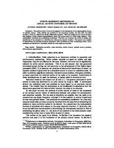
Traditionally, geometry has been represented differently in the fields of CAD and FEA. This means that the CAD geometry, which is exact, must be converted to an Analysis Suitable Geometry (ASG) for input into a FEA program. In order to obtain an ASG, features like inserts, holes and other details are often omitted to avoid numerical problems during analysis. This cumbersome process takes up to 80%[39] of the total analysis time and is generally known as ’meshing’. The need for precise geometry in analysis is obviated by Figure 1.1. Here an example is shown where spurious oscillations arise due to a crude geometric approximation with straight-sided elements. Smoothing the geometry completely eliminates the spurious oscillations even when the flow field is approximated by linear elements. Other areas for which exact geometry representation

Figure 1.1: Isodensity contours of GLS discretization of Ringleb flow. Isoparametric linear Lagrange element approximation: (a) both solution space and geometry space are represented by piecewise linear functions. (b) Superparametric element approximation: solution space is piecewise linear, while geometry space is piecewise quadratic. Smooth geometry avoids spurious entropy layers associated with piecewise linear geometric approximations. Taken from Barth [2].

is important are for example: Fluid Structure Interaction (FSI) requires a precise description of the fluid structure interface; non-linear phenomena such as transition to turbulence and buckling of thin-shell structures are extremely sensitive to small deviations in the geometry. The disparity between the fields of FEA and CAD on the subject of geometry representation is remarkable. This has mainly to do with the fact that they are seen as separate fields, which are interfaced using complicated and expensive mesh generation schemes. In order to avoid this problem, it is preferable to use an integrated approach where the CAD geometry is directly used in the FEA. Some attempts at this have been made in the recent years a few of which are highlighted in the next section. Dennis Ernens

M.Sc. Thesis

1.2 Previous attempts

1.2

3

Previous attempts

The idea to bring exact geometry to the Finite Element Method in an integrated way is not new. In 1973 Gordon and Hall [32] proposed the transfinite mapping technique to get an exact description of the computational domain [33] by using analytical functions to define the boundary of the domain. It was not a solution to the aforementioned meshing problems but did introduce exact geometry in analysis. A blend of the transfinite mapping method and NURBS can be found in the paper by Schramm and Pilkey [56]. They recognized that using NURBS for both the analysis and geometry description comes with great advantages in the design process. More recent is the approach by Cirak et al. [20] which uses subdivision surfaces1 for geometry and analysis and the work of Höllig [34], Höllig et al. [35, 36] which uses weighted B-Splines. Independently, Botella and Shariff [12] recognized the added benefit of higher inter-element continuity which the BSpline basis offers. Although all these works proved the benefits of using exact geometry and an integrated approach it really needed someone with high standing in FEA to promote these ideas.

1.3

IsoGeometric Analysis

IsoGeometric analysis was introduced in 2005 by Hughes et al. [37] to bring exact engineering geometry to Finite Element Analysis (FEA) and alleviate the cumbersome process of meshing altogether. The Isogeometric Analysis concept unifies the two fields of CAD and FEA by expanding the solution space using the same basis as that of the geometry description from CAD. Since its introduction, IGA has successfully been applied to a wide variety of problems in structural analysis [22, 38, 67], electromagnetics [17], turbulence [1, 6, 8], fluid structure interaction [4, 7, 10, 11] and higher order partial differential equations [31]. Figure 1.2 shows some results of a full FSI of a wind turbine using IGA. There are several candidate technologies available to the Isogeometric Analysis framework, of which NURBS is most commonly used since it is the standard technology employed in CAD programs. NURBS generalize B-Splines and consequently inherit all of their favourable properties for freeform design. NURBS are commonly used in Computer Aided Design (CAD), Manufacturing (CAM), and Engineering (CAE) and are part of numerous industry-wide used standards, such as IGES, STEP, ACIS, and PHIGS. NURBS are piecewise-rational functions and allow a compact representation of geometry, can be efficiently evaluated [24, 26, 54], can exactly represent some simple geometries2 like cylinders, spheres, ellipsoids and allow easy manipulation through their control points. Isogeometric Analysis based on NURBS has refinement procedures analogue to h- and p-refinement in FEA, which are respectively known as knot insertion and degree elevation. The property of splines having a high level of derivative continuity at element interfaces also gives rise to the potentially more powerful k-refinement [1, 23], where the degree is elevated together with the continuity at the element interfaces. In practise, however, pure k-refinement is generally not 1 2

Which are a bi-cubic B-Splines.[19] More generally known as quadric. http://en.wikipedia.org/wiki/Quadric

MSc. Thesis

Dennis Ernens

4

Introduction

Figure 1.2: Isocontours of air speed at a planar cut superposed with the wind turbine rotor on the deformed configuration. Rotor blade deflection is clearly visible: (a) t = 0.7 [s]; (b) t = 1.2 [s]; (c) t = 2.0 [s]; (d) t = 4.5 [s]. Taken from Bazilevs et al. [10]

possible due to geometric restrictions on the continuity. The B-Spline basis has proven to have superior dispersion properties when compared to the classic3 high order FEM basis, Chapter 5 [39] and [29, 38]. Figure 1.3 shows this for 1D wave propagation. The high frequency mode behaviour of classical FEM is divergent with the order of approximation. NURBS on the other hand offer almost spectral approximation properties and all modes converge with increasing order of approximation. These are very desirable properties in problems with 3 When referring to classic FEM I mean the collection of methods based on Lagrangian polynomials as basis functions.

Dennis Ernens

M.Sc. Thesis

1.3 IsoGeometric Analysis

5

Figure 1.3: Comparison of p-FEM with k-refined B-Splines numerical spectra for 1D free vibration, with on the y-axis the discrete-to-exact ratio of the frequencies and on the x-axis the scaled mode number. By the duality principle this is equivalent to the 1D Helmholtz equation by ωh interchanging frequency with wave number ωnn ↔ kknh . Taken from Hughes et al. [38]. n

wave propagation, long time integration and a multi-scale character. These properties are mainly ascribed to the aforementioned inter-element continuity of the basis functions.

1.3.1

Issues in IGA

Multiple dimensions are typically handled using tensor products of 1D basis functions, therefore local mesh refinement and adaptive mesh refinement (i.e. in an error estimation framework) is not possible with the global operating tensor product B-Splines. Furthermore, due to the tensor product nature it is also difficult to deal with various topological shapes. A single NURBS patch can only represent quadric shapes. Employing multiple patches seems a natural way of solving these [23] issues, although it becomes progressively more difficult with increasing p and k to produce seamless patch interfaces. The topological limitations can be solved partly by employing trimmed NURBS [42, 43, 60] or web-splines [34–36]. Alternatives to the tensor product approach which do provide local refinement capibilities are the following. T-Splines, a generalization of NURBS, are a promising technology giving the same adaptivity as quadrilateral FEM codes [9, 57, 59] with huge savings in degrees of freedom compared to NURBS. Note that T-Splines are also a solution to the topology problem, they produce seamless patch interfaces and can be combined with trimmed NURBS. However, issues remain: in certain cases the refinement algorithm operates in a non-local way leading to additional refinements propagating through the whole patch. The refinement pattern is non-unique, depending on the order in which elements are refined. The inability to locally vary p and k is also a shortcoming. Finally, linear independence is not guaranteed through the refinement process [15] but can be ensured using the procedure proposed by [50]. There is also a procedure to convert an unstructured quadrilateral mesh to a T-mesh [70]. MSc. Thesis

Dennis Ernens

6

Introduction

Multilevel/hierarchical B-Splines [45, 46] are another way to overcome the refinement issue while keeping all the standard evaluation algorithms. The hierarchical structure of the basis is exploited by combining basis functions at different levels of refinement. When refinement is needed the basis functions of a level higher become active at that location. The construction of the hierarchical basis is flexible, various combinations of hpk-refinements can be used on each refinement level. This even allows for local anisotropic refinement. Furthermore the hierarchical basis can probably facilitate a multigrid method for the solution of the linear system. Recently the first application in IGA was done by Vuong et al. [68]. A new interesting approach is that of Locally Refined splines [28] (LR-Splines). LR-Splines share some of their properties with multilevel splines and T-splines. The main difference is that in LRsplines the refinement is done by locally inserting additional knots. Unfortunately this technique is still shrouded in mystery because the only account of it is the referred conference presentation. An alternate solution are simplex based technologies which abandon NURBS as a basis for IsoGeometric Analysis. Instead, they adopt an alternative framework that does permit local mesh refinement such as simplex B-Splines or subdivision surfaces [25, 44, 66]. Although IGA alleviates the cumbersome process of meshing by directly employing the CAD geomety in analysis, even in 2D problems it is not clear how to best generate a mesh based on a CAD description of only the boundary of the domain. However, this can still be solved with the current CAD technology, a bigger challenge are 3D volume meshes. Current NURBS technology can only provide a surface representation of an object. Volumes are defined by their bounding surfaces. For IsoGeometric Analysis to become a mature technology a solid NURBS modeller is needed. The development of a threedimensional (trivariate) representation of the solid such that the surface representation is exactly preserved is not trivial. Surface differential and computational geometry are fairly well understood, but the three dimensional problem is still open. New technologies are being developed to tackle this problem, such as Ricci flows and polycube splines [49, 69]. Polycube splines have similarities with the template-based system created by Zhang et al. [73] who used a solid NURBS modeller to construct patient specific models of arteries. See for more preliminary efforts [21, 71]. Finally, IGA invokes the isoparametric concept which introduces NLTE through the mapping from the pararameter space to physical space. This mapping is non-linear when non-polygonal geometry is considered. The basis functions in physical space are therefore not polynomial. Convergence rates, however, are retained. This has been known as one of the variational crimes committed in the FEM , see [13] for a complete overview.

1.4

NURBS Enhanced Finite Element Method

The NURBS enhanced Finite Element Method (NEFEM) by Sevilla et al. [63] also unifies CAD geometry with classical FEM. There are two main differences between NEFEM and IGA. First, NEFEM considers the exact NURBS description only for the boundary of the computational Dennis Ernens

M.Sc. Thesis

1.4 NURBS Enhanced Finite Element Method

7

domain, the usual information provided by CAD software. Secondly, NEFEM circumvents NLTE by approximating the solution with a standard piecewise polynomial interpolation in Cartesian coordinates. Now the basis is polynomial in physical space, but by doing so an inconsistency arises. Due to the basis functions being polynomial they are non-zero on the boundary when it is curved. Therefore violating the requirements of the weight function space such that strong boundary conditions cannot be imposed. An elegant fix for this has been provided by Scott [58] in 1975, by placing Lobatto points on the boundary in such a way that the error of the inconsistency goes faster to zero than the approximation error. This makes the inconsistency not an issue in practise. Figure 1.4 shows the improved accuracy by employing this approach on domains with curved boundaries.

(a)

(b)

Figure 1.4: Poisson equation results on a curved domain. Here NEFEM, isoparametric FEM, p-FEM and Cartesian FEM are compared. Isoparametric FEM approximates the boundary with piecewise polynomials and has NLTE, p-FEM employs an exact boundary representation but still has NLTE and Cartesian FEM circumvents NLTE by defining the interpolation in Cartesian coordinates while approximating the boundary with piecewise polynomials. Figure 1.4(a) shows the p-refinement results for a polynomial manufactured solution of degree 7. NEFEM satisfies this patch test even on curved domains. Figure 1.4(b) shows the p-refinement results for a nonpolynomial manufactured solution. Note the improved accuracy of the NEFEM approach due to the Cartesian basis. From Sevilla et al. [62].

Moreover, every interior element (i.e. elements not having an edge or face in contact with the NURBS boundary) can be defined and treated as a standard FEM element. Therefore, in the vast majority of the domain, interpolation and numerical integration are standard, preserving the computational efficiency of the classical FEM. Specific numerical strategies for the interpolation and the numerical integration are needed only for those elements affected by the NURBS boundary representation. Furthermore NEFEM solves the aforementioned problems with local refinement and volume meshes, because NEFEM is a regular FEM on the interior, which gives it a strong advantage over IGA. Standard (adaptive) refinement schemes can be directly applied without the need to refine for the geometry and at most a NURBS boundary representation is needed, removing the MSc. Thesis

Dennis Ernens

8

Introduction

need for a NURBS volume mesher and it allows NEFEM to exploit standard unstructured meshing technology. However, the change to the Lagrange basis makes NEFEM lose the favourable dispersion properties of the B-Spline basis.

1.5

AnisoGeometric Analysis

The AnisoGeometric Analysis (AGA) approach was developed during the graduation period together with René Hiemstra and is inspired by the ideas of NEFEM and IGA. AGA employs exact NURBS geometry with an arbitrary choice for the solution space basis. The decoupling of the solution space from the geometry space lifts the restrictions imposed by the continuity of the geometry enabling pure k-refinement, which will be referred to as ”high regularity approaches”. Here AGA is presented with a B-Spline basis and a Lagrange basis, but can in principal be applied to any type of element/basis function. Furthermore, hybrid approaches can be constructed using B-Splines in the interior for favourable dispersion characteristics and NEFEM elements on the boundary to avoid NLTE. When using a B-Spline basis for the solution space, higher regularity approaches are not limited by the continuity of the geometry. Potentially saving a considerable amount of degrees of freedom. Furthermore, Gauss quadrature is exact and efficient when piecewise polynomial B-Splines are used. This work will show that on smooth geometry (C 1 and above) this approach potentially gives the same accuracy as IGA up to a certain difference between geometric and solution space continuity, while retaining optimal convergence rates. When choosing a Lagrange basis for the solution space, AGA can be easily applied to an existing FEM code. In fact, only an additional Jacobian evaluation needs to be added in the assembly process. It turns out that Lagrange-based AGA reaches optimal convergence rates in all test problems and is competitive with NEFEM for lower-degree approximations. Furthermore Lagrangebased AGA also solves the aforementioned problems with local refinement, although without the favourable dispersion properties of IGA.

1.6

Test cases

The test cases used throughout this thesis are Poisson problems, furthermore a convection-diffusion problem will be introduced in Chapter 3. The source terms are found by the method of manufactured solutions. Hence the following equation is solved −∆u(x, y) = f (x, y)

u(x, y) = Iu(x, y) = g(x, y)

∇u(x, y) · n = h(x, y) Dennis Ernens

∈Ω

∈ Γd

∈ Γn

(1.1) M.Sc. Thesis

1.7 Goal of the thesis

9

where Ω is the physical domain, Γd ∪ Γn = ∂Ω and n is the outward unit normal on ∂Ω. The manufactured solutions used in this thesis are the following u(x, y) = x5 − 5x3 y 2 − 3y 5

f (x, y) = −20x3 + 70y 3 + 30yx2

(1.2a)

u(x, y) = x cos (y) + y sin (x) f (x, y) = x cos (y) + y sin (x)

(1.2b)

u(x, y) = sin (kπx) sin (kπy) f (x, y) = 2(kπ)2 sin (kπx) sin (kπy) −(x2 + y 2 ) u(x, y) = exp 0.02 −(x2 + y 2 ) f (x, y) = 200 exp −1 + 50x2 + 50y 2 0.02

(1.2c)

(1.2d)

where the Dirichlet boundary conditions are found by interpolation. Case (1.2b) is taken from Sevilla et al. [63] and case (1.2d) will √ be used to test adaptive refinement. When comparing results the L2 -norm versus hmax or ndof is used to define the quality of the solution. √ Where hmax is defined as the maximum circumdiameter of the element in physical space and ndof is the square root of the number of degrees of freedom.

1.7

Goal of the thesis

The goal of this thesis is to quantify and clarify some of the limitations of IGA, NEFEM and AGA. These include the effect of non-linear transformation error on the higher continuity approaches. It is known from the previous sections of this chapter that Cartesian Lagrange bases remove this error, improving the accuracy of the approximation. On the other hand, the higher inter-element continuity of the B-Spline basis is also known to increase the accuracy of the approximation by giving superior dispersion characteristics when compared to those of the Lagrange basis. In this thesis the following research questions are answered: • How detrimental is NLTE opposed to the beneficial properties of higher continuity B-Splines in steady problems? • Are there any benefits in combining the ideas of IGA and NEFEM in AGA? Furthermore this thesis will clarify some of the limitations of IGA and NEFEM which are not found in literature. MSc. Thesis

Dennis Ernens

10

1.8

Introduction

Structure of the thesis

The structure of the thesis is as follows. Chapter 2 will start with the necessary theory on B-Splines and NURBS and acts as a prelude for the proceeding chapter(s). Then, refinement strategies for the B-Spline basis are demonstrated and limitations of NURBS in an analysis framework are discussed. Next, in Chapter 3, will show the development of a NURBS based FEM for the convection-diffusion equation. Numerical experiments are performed on the convection-diffusion equation and the Poisson equation. Some observations are made on the conditioning of the linear system as well as some counterintuitive NURBS results. Chapter 4 will describe the NURBS Enhanced Finite Element Method. This method also uses NURBS for the geometry definition but represents its field variables using Lagrange polynomials. Here the focus is on the development of boundary elements and their basis functions. NEFEM avoids non-linear transformation errors but in doing so an inconsistency arises. Attempts at fixing this inconsistency are the main topic of this chapter. Numerical experiments will show the superior accuracy on curved geometry which can be attained by using a NEFEM approach. Then the AnisoGeometric method developed during the course of this thesis is presented in Chapter 5. The development is shown for both B-Splines and Lagrange polynomials. In Chapter 6 the potential of AnisoGeometric Analysis is shown using numerical experiments, and a comparison between IGA, NEFEM and AGA is made. Conclusions and recommendations will be given in Chapter 7.

Dennis Ernens

M.Sc. Thesis

Chapter 2 B-Splines and NURBS 2.1

Introductory remarks

In this chapter B-Splines and NURBS are introduced as a compact and elegant way to describe geometry. This chapter will show the reasons why splines are an attractive basis, not only for CAD but also in an analysis framework. To this end some observations are already made in the light of analysis with splines, as preliminary for Chapter 3. The chapter starts with a brief history and the definition of the parametric space and the B-Spline basis functions which live there. Subsequently the construction of curves, surfaces and volumes will be addressed. The possibilities to refine the basis will be discussed thereafter. The generalization to NURBS is made in Section 2.5. In this chapter the notation of Hughes et al. [39] combined with Piegl and Tiller [54] is used. Other important references for this chapter are the works by [24, 26, 27, 48, 55, 69].

2.2

Brief history

Historically splines were first used for shipbuilding before the age of computer modelling. Naval architects used splines, which were thin bendable strokes of wood, to draw smooth curves for the lines plan of the ship. Metal weights, called ducks, were placed such that the spline had its preferred shape. In between the ducks the spline will assume shapes of minimum strain energy leading to smooth curvature continuous (C 2 ) geometry everywhere, see also Figure 2.1. With the advent of the computer, Computer Aided Geometric Design (CAGD) emerged. CAGD is concerned with the generation of smooth curves and surfaces, which generally have to satisfy a large number of constraints. When using polynomials this requires high degree approximations because degree p polynomials can satisfy p + 1 constraints. High degree polynomials are inefficient to process, can become unstable and have the disadvantage that changes are global, while local MSc. Thesis

Dennis Ernens

12

B-Splines and NURBS

Figure 2.1: A spline held by ducks to obtain the required smooth design shape.

control is needed. In addition, continuity should be maintained when local changes are made. These issues were overcome by the definition of a Spline in the mathematical sense, a function constructed from polynomial elements pieced together with a certain level of continuity between the elements. The required continuity is directly built into the basis which made Basis Splines or B-Splines, the natural basis in which to define splines, such a success in CAGD. The B-Spline basis allows an arbitrary choice of continuity between the elements from C 0 to maximum C p−1 . Curvature continuity is an important requirement in design, because it guarantees a smooth change of reflections. Cubic Splines are therefore most commonly used in CAGD. B-Splines are convenient for free-form modelling, but they lack the ability to exactly represent some simple engineering shapes like circles and ellipsoids. This is why today, the de facto standard technology in CAD is a generalization of B-Splines called NURBS. NURBS stands for Non-Uniform Rational B-Splines, they are rational functions of B-Splines and inherit all their favourable properties. NURBS extend B-Splines since they allow exact representation of conic sections. For a full account on the history of curves and surfaces in CAGD the interested reader is referred to [30].

2.3

B-Splines

The natural starting point for a discussion about NURBS are B-Splines, remember NURBS are built from B-Splines.

2.3.1

Parameter domain

B-splines are defined on a parameter space Ω′ . The B-Spline parameter space is local to ”patches” instead of elements, where the patch can be seen as a ”macro-element”. The parameter domain itself is defined by the knot vector(s) Ξ. The knot vector is defined as Ξ = {(ξ1 , . . . , ξp+1 = a) , ξp+2 , . . . , ξn , (ξn+1 , . . . , ξn+p+1 = b)} Dennis Ernens

M.Sc. Thesis

2.3 B-Splines

13

where, ξi ∈ R is the ith knot, i is the knot index, i = 1, 2, . . . , n + p + 1 and n equals the number of basis functions. Higher dimensional parameter spaces are constructed using a tensor product of 1D knot vectors. Hence the parameter domains are defined by the set [a, b]d ∈ Rd with d the dimension of the space. Using the knot vector one can construct B-spline basis functions of order p + 1 which are piecewise polynomials of degree p. Repeated knots are allowed, hence ξ1 ≤ ξ ≤ . . . ≤ ξn+p+1 . A knot that is repeated k times is said to have a multiplicity k. Remark 2.3.1: (1) There is a clear distinction between order and degree in the definition of the knot vector. This thesis obeys the computational geometry convention that order is degree plus one or o = p + 1. (2) The knots can be equally spaced giving a uniform knot vector, unequally spaced knots consequently give a non-uniform knot vector. (3) The knot vector is open, meaning that, the first p + 1 and last p + 1 knots are repeated. The implications of repeated knots will become clear in Section 2.3.2. (4) Note that we can define an element or knot span in the parameter domain as [ξi , ξi+1 ).

2.3.2

B-Spline basis functions

The B-Spline basis functions are defined recursively starting with piecewise constants ( 1 if ξi ≤ ξ < ξi+1 Bi,0 (ξ) = 0 otherwise.

(2.1)

For p = 1, 2, 3, . . . , the definition is Bi,p (ξ) =

ξ − ξi ξi+p+1 − ξ Bi,p−1 (ξ) + Bi+1,p−1 (ξ). ξi+p − ξi ξi+p+1 − ξi+1

(2.2)

So given a knot vector and a polynomial degree the B-Spline function space B is uniquely defined as B ≡ B(Ξ; p) := span {Bi,p }ni=1 by using the recursive algorithm. Higher-dimensional B-Spline function spaces are constructed using tensor products of univariate B-Spline basis functions namely B ≡ B(Ξ, H, . . . ; p, q, . . .) := span {Bi,p ⊗ Bj,q ⊗ . . .}n,m,... i,j,...=1 .

(2.3)

The result of (2.1) and (2.2) is shown in Figure 2.2 for the knot vector Ξ = {0, 0, 0, 0, 1, 2, 3, 4, 4, 4, 4}. An example of a quadratic basis for an open, non-uniform knot vector is shown in Figure 2.3. Here the implications of the repeated knots at the ends of the interval and also at ξ = 4 are shown, where the continuity is lowered to C 0 . The other basis functions MSc. Thesis

Dennis Ernens

14

B-Splines and NURBS B1,3

1

B3,1

1

B4,0

1 0

0

1

2

0

1

2

3

0

1

2

3

1 0

4

4

B6,0

1 0

3

B5,0

1 0

·

0

1

2

3

µ

1−ξ 1−0

¶

+0 0

µ

¶ ξ −1 +1 µ2 − 1¶ 3−ξ · +0 0 3−2

·

4

·

·

2

1

2

ξ −3 4−3

¶

4

0

4

B5,1 1

2

3

4

B6,1 1

2

+1 0

3

1

2

µ

1−ξ 1−0

¶

+0 0

µ

¶ ξ −0 +1 µ1 − 0 ¶ 2−ξ · +0 0 2−0

1

¶ ξ −1 +1 µ3 − 1¶ 4−ξ · +0 0 4−2

·

3

4

4

·

·

ξ −3 4−3

¶

3

1

2

0

4

3

4

B5,2 1

2

1

2

1

2

1−ξ 1−0

¶

+0 0

3

4

µ

¶ ξ −0 +1 µ2 − 0¶ 3−ξ +0 0 · 3−0

·

·

3

4

·

·

3

4

2

3

4

2

3

4

3

4

B3,3 1

µ

¶ ξ −0 +1 µ3 − 0¶ 4−ξ · +0 0 4−1 ·

2

µ

B4,3 1

2

µ

¶ ξ −2 +1 µ4 − 2¶ 4−ξ · +0 0 4−3 B7,2 4

1

¶ ξ −0 +1 B2,3 µ1 − 0¶ 2−ξ +0 0 · 1 2−0

·

¶ ξ −1 +1 µ 4 − 1¶ 4−ξ · +0 0 4−2 B6,2

3

+1 0

4

B4,2

µ

µ

3

2

µ

¶ ξ −2 +1 µ4 − 2¶ 4−ξ 0 B7,1 · 4 − 3 + 0

3

1

¶

µ

2

B3,2

ξ −0 +1 2−0 µ ¶ 3−ξ · + 00 3−1 ·

µ

µ

3

B4,1

µ

¶ ξ −2 +1 µ 3 − 2¶ 4−ξ 0 B7,0 · 4 − 3 + 0 4

1

·

¶ ξ −0 +1 µ1 − 0¶ 2−ξ +0 0 · 2−1

·

·

·

B2,2

1

µ

B5,3 1

2

µ

µ

ξ −3 4−3

¶

3

B6,3 1

2

3

4

B7,3

+1 0

4

0

1

2

3

4

Figure 2.2: Recursive generation of a cubic basis for the uniform knot vector Ξ = {0, 0, 0, 0, 1, 2, 3, 4, 4, 4, 4}.

are C 1 continuous. Degree p basis functions have up to p − 1 continuous derivatives. A repeated knot will reduce the number of continuous derivatives by 1. When the multiplicity equals p, the basis function is nodal. The basis functions possess the following important properties: 1. Non-negativity: Bi,p (ξ) ≥ 0 ∀i, p and

a ≤ ξ ≤ b.

2. On a knot span [ξi , ξi+1 ) there are p + 1 non-zero functions. Pn 3. Partition of unity. i=1 Bi,p (ξ) = 1.

4. The basis functions form a linear independent basis which makes them suitable for analysis.

5. B0,p (0) ≡ Bn,p (1) ≡ 1. 6. Compact support [ξi , ξi+p+1 ). Higher order functions have support across larger portions of the domain. This increase in support has no implications on the bandwidth of the resulting linear system in numerical applications. The total number of functions that any function Dennis Ernens

M.Sc. Thesis

2.3 B-Splines

1

15

B3,2

B4,2

B5,2

B6,2

B8,2 B7,2

Bi,2

B1,2 B 2,2

0

0

1

2

3

4

5

ξ Figure 2.3: Quadratic basis {0, 0, 0, 1, 2, 3, 4, 4, 5, 5, 5}.

functions

for

the

non-uniform

knot

vector

Ξ

=

shares support with (including the function itself) is 2p+1 which is equal to that for Lagrange polynomials.

control polygon p=2 p=4 p=6

Figure 2.4: Variation diminishing property depicted for increasing curve degree.

MSc. Thesis

Dennis Ernens

16

B-Splines and NURBS

2.3.3

B-Spline derivatives

Derivatives of B-Spline basis functions are generated using the B-Spline lower order bases k

X dk p! αk,j Bi+j,p−k (ξ), B (ξ) = i,p dξ k (n − p)! j=0

with α0,0 = 1 αk−1,0 ξi+p−k+1 − ξi αk−1,j − αk−1,j−1 = ξi+p+j−k+1 − ξi+j −αk−1,k−1 . = ξi+p+1 − ξi+k

αk,0 = αk,j αk,k

j = 1, . . . , k − 1

When the denominator becomes zero due to repeated knots, the coefficient is defined to be zero.1

2.3.4

B-Spline curves

B-Spline curves are defined by the coefficients of the basis functions, the control points Pi . The curve is constructed in Rd by taking linear combinations of a set of n basis functions Bi,p , i = 1, 2, . . . , n , with their corresponding control points Pi ∈ Rd , i = 1, 2, . . . , n. The piecewisepolynomial B-Spline curve is given by C(ξ) =

n X

Bi,p (ξ)Pi

i=1

a ≤ ξ ≤ b.

(2.4)

Hence given a degree p, a knot vector Ξ and set of control points Pi the curve is defined. The curve C(ξ) is a vector-valued function of one parameter. It maps a line segment into Euclidean 3D space or more formally C : Ω′ → Ω, this is shown graphically in Figure 2.5. Figure 2.6(b) shows an example of a curve using the basis functions considered in Figure 2.3. Note that the curve, like its basis, is interpolatory at the first and last control point due to the open knot vector and at control point P6 due to the multiplicity of ξ = 4. Furthermore the curve is tangent to the control polygon at the first, last and sixth control point. The derivative of a curve can be easily computed using the derivatives of the basis functions, like ′

C (ξ) =

n X dBi,p (ξ) i=1

dξ

Pi

a ≤ ξ ≤ b.

B-Spline curves posses the following important properties: 1

For algorithms see Piegl and Tiller [54].

Dennis Ernens

M.Sc. Thesis

2.3 B-Splines

17 P8

5

B 8,2 P7

B7,2

P7 : (1, 3) B6,2

4

3

P6

elements controlpoints knots

P5 B5,2 3

P3 : (1, 2)

ξ

2

B 4,2

P4

B3,2

P3

y

2

P6 : (3, 2)

P8 : (0, 2)

1

P4 : (2, 1)

1

P5 : (3, 1)

P2 : (0, 1)

B2,2 P2 B1,2 0

0

1

Bi,2

(a)

P1

P1 : (1, 0) 0

0

1

2

x

3

(b)

Figure 2.5: The creation of a curve. Figure 2.5(a) shows the parameter domain Ω′ together with the control net P. Taking linear combinations of the basis with the control net (2.4) results in the curve in Figure 2.5(b).

1. The properties of the B-spline curve follow directly from the properties of the B-spline basis functions. Like its basis a B-spline curve of degree p has p − 1 continuous derivatives in the absence of repeated knots or control points. Another important property is that the compact support of the basis gets passed on to the curve. Thus moving a single control point does not affect more then p + 1 elements of the curve.

2. Repeating a knot or control point k times, reduces the number of continuous derivatives by k.

3. Non-negativity of the basis leads to the convex hull property, if ξ ∈ [ξi , ξi+1 ) then C(ξ) lies within the convex hull of the control points Pi−p , . . . , Pi .

4. Variation diminishing property with increasing degree. Figure 2.4 shows this property for increasing degree. The curve will never wiggle more than its control polygon, hence the spectral content of the curve is at most equal to the spectral content of the data. See Section 3.4.4 for a discussion on the implications of this property in analysis.

5. Affine invariance property. Affine transformations of a B-spline curve are applied to the control points directly. MSc. Thesis

Dennis Ernens

18

B-Splines and NURBS 4

P2

P3

controlpoints

3

knots

C(ξ)

P5 2

P1

1

knots

P5 2

1

P6

P1

P6

0

1

2

3

4

0

5

0

1

2

ξ B i,3

B1,2

0

B3,2

B2,2

0

1

B4,2

2

3

4

5

ξ B5,2

B6,2

1

B 7,2

B1,2

B i,2

1

P7

P4

P4 0

P8

elements

P2

controlpoints

P3

3

C(ξ)

4

P7

elements

3

4

5

0

B3,2

B2,2

0

1

B4,2

2

B 5,2

3

B 8,2 B6,2 B 7,2

4

5

ξ

ξ

(a) p = 2, Ξ = {0, 0, 0, 1, 2, 3, 4, 5, 5, 5}

(b) p = 2, Ξ = {0, 0, 0, 1, 2, 3, 4, 4, 5, 5, 5}

Figure 2.6: Figure 2.6(a) shows a quadratic curve with a uniform knot vector. Figure 2.6(b) shows a curve where ξ = 4 has a multiplicity of k = 2. Note the reduced continuity of the curve at P6 due to the multiplicity of ξ = 4.

2.3.5

B-Spline surfaces and solids

The B-Spline surface is defined by a control net Pij , i = 1, 2, . . . , n, j = 1, 2, . . . , m and the knot vectors Ξ = {ξ1 , ξ2 , . . . , ξn+p+1 } , H = {η1 , η2 , . . . , ηm+q+1 } . Taking the tensor product of the univariate basis functions Bi,p (ξ) and Bj,q (η) with the control net results in a B-Spline surface defined as S : Ω′ → Ω with the map defined as S(ξ, η) =

n,m X

Bi,p (ξ)Bj,q (η)Pi,j .

i=1,j=1

It is important to note that the univariate functions are defined on their own knot vector, hence they can have a different parametrization. Furthermore a different degree can be chosen for each coordinate direction. Analogous to B-Spline surfaces, B-Spline solids are defined as the tensor product of three univariate basis functions. Given a control net Pi,j,k , i = 1, 2, . . . , n, j = 1, 2, . . . , m, k = 1, 2, . . . , l and knot vectors Ξ = {ξ1 , ξ2 , . . . , ξn+p+1 } , H = {η1 , η2 , . . . , ηm+q+1 } and Z = {ζ1 , ζ2 , . . . , ζl+r+1 } , the B-Spline solid is defined as V : Ω′ → Ω with the map defined as V (ξ, η, ζ) =

n,m,l X

Bi,p (ξ)Bj,q (η)Bk,r (ζ)Pi,j,k .

i=1,j=1,k=1

2.3.6

Global curve interpolation

In order to be able to impose Dirichlet conditions a form of interpolation is needed. To this end global curve interpolation is used [54]. When using Lagrange polynomials the Dirichlet condition Dennis Ernens

M.Sc. Thesis

2.4 Refinement

19

can be directly imposed at the nodes. Because B-Splines are not interpolatory a system needs to be solved to find the right control points such that the Dirichlet condition is interpolated in the right way. For the interpolation a set of interpolation points needs to be chosen. The Greville abscissae or Marsden-Schoenberg points are the standard choice [27] and defined as the average of p consecutive knot values, viz ξj∗

p+j+1 X 1 = ξi . p+1 i=j+1

The Greville abscissae coincide with the location of the control points in parameter space. Hence they are an ideal choice for interpolation purposes. Now given a known function g(x), knot vector Ξ and map x = C(ξ) from our B-Spline or NURBS geometry global curve interpolation is defined as g

C(ξj∗ )

=

n X

Bi,p (ξj∗ )gi .

(2.5)

i=1

This results in a solvable n×n system of linear equations. For a surface repeated curve interpolation can be used, see [54] for details.

2.4

Refinement

The B-Spline basis can be enriched by three types of refinement of which two have an analogue in standard FEM bases. These are knot insertion, degree elevation and degree and continuity elevation. The first two are equivalent to h- and p-refinement respectively, the last one is dubbed k-refinement and has no equivalent in standard FEM. In this section these three enrichments are discussed and examples are shown.

2.4.1

Knot insertion: h-refinement

Knot insertion or h-refinement in classical FEM nomenclature enriches the basis by increasing the resolution of the parameter space. Given a knot vector Ξ = {ξ1 , ξ2 , . . . , ξn+p+1 } and introducing ¯ ¯ ¯ The new an extended knot vector Ξ = ξ1 = ξ1 , ξ¯2 , . . . , ξ¯n+m+p+1 = ξ¯n+p+1 such that Ξ ⊂ Ξ. ¯ n + m basis functions are formed by (2.1) and (2.2) by applying them to Ξ. The new n + m ¯ 1, P ¯ 2, . . . , P ¯ n+m T , are formed from linear combinations of the original control points, P¯ = P control points, P = {P1 , P2 , . . . , Pn }T , by ¯ = αi Pi + (1 − α) Pi−1 P MSc. Thesis

(2.6) Dennis Ernens

20

B-Splines and NURBS

where

αi =

  1,

¯ i ξ−ξ ,  ξi+p −ξi



0,

1 ≤ i ≤ k − p,

k − p + 1 ≤ i ≤ k,

(2.7)

k + 1 ≤ i ≤ n + p + 2.

Note that choosing the control points as in (2.6) and (2.7) the continuity of the curve is preserved. Figure 2.7 gives an example of knot insertion. The initial knot vector is Ξ = {0, 0, 0, 0, 1, 2, 3, 4, 4, 4, 4}, a new knot is inserted at ξ¯ = 2.5. The curve with its old and new control polygon is shown in Figure 2.7(a). The new curve is geometrically identical to the original curve, but the basis functions and control points are changed. The new knot added one basis function, compare Figure 2.7(b) with Figure 2.7(c), and one control point. Remark 2.4.1: Next to increasing the resolution of the parameter space, knot insertion can also be used to control the continuity of the basis by repeating knots. This is one of the distinguishing features of the spline basis compared with the classical FEM basis.

2.4.2

Degree elevation: p-refinement

Degree elevation is the second method of enriching the basis and is the equivalent of p-refinement in regular FEM. This procedure starts by effectively subdividing the curve into Bézier elements by knot insertion, (2.6) and (2.7), to raise the multiplicity to the polynomial degree. Then the order of the polynomial is raised on each individual segment. Finally excess knots are removed to create the new B-spline. Recall from Section 2.3.2 that the basis has p − k continuous derivatives, so increasing p also implies increasing k. This ensures that the basis keeps its original continuity. As with h-refinement the solution space spanned by the degree elevated basis functions contains the space spanned by the original functions. So it is possible to degree elevate without changing the geometry of the B-Spline curve. An example of degree elevation is given in Figure 2.8. Again the starting point is a cubic curve with the control net P and basis functions shown in Figure 2.8(a) and Figure 2.8(b) respectively. After degree elevation the multiplicity of the knots is increased by ¯ change. Though, the elevated curve one and consequently the locations of the control points, P, is still geometrically and parametrically the same. Figure 2.8(c) shows the enriched basis, there are now 11 quartic basis functions. Remark 2.4.2: (1) Note that unlike knot insertion, degree elevation is a global process.

2.4.3

Continuity and degree elevation: k-refinement

A potentially more powerful type of refinement which is unique to the B-Spline basis is krefinement. Basically k-refinement is a different order elevation strategy taking advantage of the fact that knot insertion and degree elevation do not commute. Inserting a unique knot value Dennis Ernens

M.Sc. Thesis

2.4 Refinement

21

¯ 3 = P3 P

¯4 P

2

P4

¯5 P

y

1

0

¯ 1 = P1 P

P5

¯ 2 = P2 P

¯6 P

¯ 8 = P7 P elements

−1

old control points knots new control points

¯ 7 = P6 P

inserted knots −2

0

1

2

3

x

4

5

(a) Curve with old and new control points due to knot insertion. 1

B3,3

B4,3

1

B7,3 B6,3

B5,3

B 1,3 B2,3

B i,3

Bi,3

B1,3 B2,3

0

0

1

2

3

4

ξ

(b) Initial basis functions: {0, 0, 0, 0, 1, 2, 3, 4, 4, 4, 4}.

0

0

B 3,3

1

B 8,3

B5,3

B4,3

B6,3

2

B 7,3

3

4

ξ

p

=

3,

Ξ

= (c) New basis functions: p {0, 0, 0, 0, 1, 2, 2.5, 3, 4, 4, 4, 4}.

=

3,

¯ Ξ

=

Figure 2.7: Figure 2.7(a) shows an example of knot insertion performed on a cubic B-Spline curve defined by the initial knot vector Ξ = {0, 0, 0, 0, 1, 2, 3, 4, 4, 4, 4} and control net P. The basis functions defined by Ξ are shown in Figure 2.7(b). Inserting the knot ξ¯ = 2.5 results in an additional control point and basis function as shown in Figure 2.7(a) and Figure 2.7(c) respectively.

MSc. Thesis

Dennis Ernens

22

B-Splines and NURBS

¯5 P

P3

P4

2

¯6 P

¯4 P

¯7 P

1

y

¯3 P 0

¯8 P ¯ 1 = P1 P

¯2 P

P5

P2

¯ 11 = P7 P −1 elements

¯9 P

old control points knots

¯ 10 P

new control points −2

0

1

2

P6 3

x

4

5

(a) Curve with old and new control points due to degree elevation. 1

B3,3

B4,3

B5,3

1

B7,3 B6,3

B 1,4 B2,4

B i,4

Bi,3

B1,3 B2,3

0

0

1

2

3

4

ξ

(b) Initial basis functions: {0, 0, 0, 0, 1, 2, 3, 4, 4, 4, 4}

0

0

B11,4 B3,4

B 7,4

B 5,4 B4,4

1

B6,4

2

B 8,4

B9,4

B10,4

3

4

ξ

p

=

3, Ξ

= (c) New basis functions: p = {0, 0, 0, 0, 0, 1, 1, 2, 2, 3, 3, 4, 4, 4, 4, 4}

¯ 4, Ξ

=

Figure 2.8: Figure 2.8(a) shows a degree elevation of a cubic B-Spline curve defined by the initial knot vector Ξ = {0, 0, 0, 0, 1, 2, 3, 4, 4, 4, 4} and control net P. The basis functions defined by Ξ are shown in Figure 2.8(b). The degree elevation results in a quartic curve with the enriched ¯ = {0, 0, 0, 0, 0, 1, 1, 2, 2, 3, 3, 4, 4, 4, 4, 4} and control net P. ¯ The enriched basis is knot vector Ξ shown in Figure 2.8(c).

Dennis Ernens

M.Sc. Thesis

2.4 Refinement

23

ξ¯ between two distinct knots in a degree p curve lowers the number of continuous derivatives at ξ¯ to p − 1. Elevating the degree to q, using the process of Section 2.4.2, increases the multiplicity of each knot so that discontinuities in the pth derivative of the basis are preserved. Hence the ¯ The above process can be turned around by basis still has p − 1 continuous derivatives at ξ. ¯ Now the basis has first elevating the curve degree to q and then inserting the unique knot ξ. ¯ This process is called k-refinement and has, as said before, no q − 1 continuous derivatives at ξ. analogue in classical FEM. By enriching the basis using k-refinement there is also the potential to save a significant amount of degrees of freedom. Consider again the previous example but this time keeping track of the number of basis functions, see also Figure 2.9. Lets start with a single element2 of degree p, this element has p + 1 basis functions. Then perform knot insertion to arrive at n − p elements with a total of n basis functions. Like before elevate the degree keeping the continuity p − 1 by increasing the multiplicity of each knot by one. This adds a basis function per element, hence the total number of basis functions is now 2n − p. After r degree elevations the number of basis functions has become (r + 1)n − rp. This is a large number because in practice the number of elements surpasses the polynomial degree by multiple orders of magnitude. Repeating this process using k-refinement starting again with one element and p+1 basis functions. First elevate the degree r times adding one basis function each time and then insert knots until the number of elements is n − p. This results in n + r basis functions all having r + p − 1 continuous derivatives. Note that n + r ≪ (r + 1)n − rp especially when going to higher dimensions, then these get raised to the dth power namely (n + r)d ≪ ((r + 1)n − rp)d . Furthermore k-refinement adds the benefit of smoother derivatives leading to more accurate representation of physical quantities. Some examples are: the representation of the structure of bones for a smooth transition from the solid outer part to the softer inner part [52]; the representation of structural vibration modes resulting in converging spectra [22, 38, 47]; enabling the use of higher order gradient damage models [67]; removing the need for second derivative reconstruction in the momentum residual of the VMS method [1, 6]. Remark 2.4.3: (1) It is important to note that the highest continuity of the B-Spline basis is limited by the continuity of the basis of the geometrical domain of interest. Hence highest regularity BSplines are only attained for simple geometries. (2) When a physical situation requires a lower level of continuity at a knot value, it is always possible to increase the multiplicity of that knot value.

2

which is equivalent to a Bézier element.

MSc. Thesis

Dennis Ernens

24

B-Splines and NURBS

Figure 2.9: k-refinement versus p-refinement. (a) Starting with one linear element. (b) Classic p-refinement approach, knot insertion followed by degree elevation results in seven piecewise quadratic basis functions that are C 0 at the internal knots. (c) k-refinement approach, degree elevation followed by knot insertion results in five piecewise quadratic basis functions that are C 1 at the internal knots.

Dennis Ernens

M.Sc. Thesis

2.5 Non-Uniform Rational B-Splines

2.5

25

Non-Uniform Rational B-Splines

B-splines have their rational counterparts giving the ability to exactly represent objects that cannot be represented by polynomials. For example in CAD circular and conic shapes are often used, which can be exactly represented by NURBS.

2.5.1

NURBS basis functions

The NURBS basis is defined by associating the B-spline basis functions with a strictly positive weight, wi as Ni,p (ξ) =

wi Bi,p (ξ) W (ξ)

(2.8)

where W (ξ) =

n X

wi Bi,p (ξ)

i=1

spanning the NURBS function space uniquely defined as N ≡ N (Ξ; p; w) := span {Ni,p }ni=1 . Analogous to B-Splines higher dimensional function spaces are constructed using tensor products of univariate basis functions N ≡ N (Ξ, H, . . . ; p, q, . . . ; w) := span {Ni,p ⊗ Nj,q ⊗ . . .}n,m,... i,j,...=1 . The NURBS basis has the following properties: 1. The NURBS basis constitutes a partition of unity

Pn

i=1 Ni,p (ξ)

= 1 ∀ξ.

2. NURBS inherit their properties from the B-Spline basis functions like continuity across knots, local support and non-negativity. 3. The NURBS basis functions are not polynomial but rational functions. 4. If the weights are all equal the basis is again polynomial. Hence, B-Splines are a special case of NURBS.

2.5.2

NURBS derivatives

NURBS derivatives are found by using the quotient rule on (2.8), expressing the derivative in the B-Spline basis, namely ′

′

W (ξ)Bi,p (ξ) − W (ξ)Bi,p (ξ) d Ni,p (ξ) = wi dξ (W (ξ))2 P ′ ′ ′ d Bi,p (ξ) and W (ξ) = ˆni Bî,p (ξ)wî . Now define where Bi,p (ξ) ≡ dξ (k)

Ai (ξ) = wi

MSc. Thesis

dk Bi,p (ξ), dξ k

no sum on i

Dennis Ernens

26

B-Splines and NURBS

and let W (k) (ξ) =

dk W (ξ). dξ k

Then higher order derivatives are expressed in terms of lower order derivatives as (k)

Ai (ξ) − dk Ni,p (ξ) = k dξ

k (j) d(k−j) (ξ) dξ (k−j) Ni,p (ξ) j=1 j W

Pk

W (ξ)

,

where k k! . = j!(k − j)! j Efficient algorithms for the evaluation of NURBS and their derivatives can be found in [54].

2.5.3

NURBS curves

Using (2.8) the NURBS curve can be defined in the same way as the B-Spline curve namely C(ξ) =

n X

Ni,p (ξ)Pi .

i=1

Figure 2.10 shows the construction of a circular arc. Note that one weight has the value √12 to allow exact representation of the circle. The dashed line shows the curve when all weights are equal to one and hence this curve is polynomial. Comparing the two curves it is clear that due to the weight the middle control point pulls the curve less strong. P3 P2 : (0, 1) 1 w2 = √ 2

P3 : (1, 1) w3 = 1

P2

P1 : (0, 0) w1 = 1 P1

Figure 2.10: Example of the construction of a NURBS quarter circle curve based on the knot vector Ξ = {0, 0, 0, 1, 1, 1}. The dashed line indicates the unweighed curve.

Dennis Ernens

M.Sc. Thesis

2.5 Non-Uniform Rational B-Splines

2.5.4

27

NURBS surfaces and solids

In an analogous way the NURBS surface and NURBS solid are defined as

S(ξ, η) =

n,m X

Ni,p (ξ)Nj,q (η)Pi,j ,

(2.9)

i=1,j=1

V (ξ, η, ζ) =

n,m,l X

Ni,p (ξ)Nj,q (η)Nk,r (ζ)Pi,j,k .

i=1,j=1,k=1

Figure 2.11 shows the construction of a circular surface by a mapping from parameter space to physical space using the control points and weights of the circular arc, Figure 2.10, for each side of the parameter space forming a circular surface in physical space. P21 : (−1, 1) 1 w21 = √ 2

P11 : (−1, 0) w11 = 1

P12 : (−1, −1)

1 w12 = √ 2

P31 : (0, 1) w31 = 1

P22 : (0, 0) w22 = 1

P13 : (0, −1) w13 = 1

P32 : (1, 1) 1 w32 = √ 2

P33 : (1, 0) w33 = 1

P23 : (1, −1) 1 w23 = √ 2

Figure 2.11: Construction of a circle using NURBS. The surface is constructed using the knot vectors Ξ = H = {0, 0, 0, 1, 1, 1} and control points and weights as shown in the figure.

MSc. Thesis

Dennis Ernens

28

B-Splines and NURBS

2.6

Summary

• B-Spline basis functions are easily computed using the Cox-de Boor algorithm; • B-Spline derivatives are easily computed using the B-Spline lower degree bases; • B-Spline curves, surface and solids are defined by their degree(s), knot vector(s) and control net; • B-Splines have refinement procedures analogue to classical FEM, namely h-refinement and p-refinement. The k-refinement procedure is unique to B-Spline and gives the possibility to raise both the degree and continuity of the basis; • Because a B-Spline curve does not interpolate its control points a system needs to be solved to find the control points for interpolation; • NURBS basis functions are defined by associating the B-Spline basis functions with a strictly positive weight; • NURBS derivatives are found by the quotient rule expressing them in the B-Spline basis. Higher order derivatives can be expressed in terms of lower degree derivatives; • NURBS curves, surface and solids are defined by their degree(s), knot vector(s), weight(s) and control net;

Dennis Ernens

M.Sc. Thesis

Chapter 3 Isogeometric Analysis: NURBS as a basis for analysis 3.1


This chapter describes the Isogeometric Paradigm introduced by Hughes et al. [37]. For FEM practitioners this chapter can feel a bit redundant as most of the changes are nomenclature based and characteristic for the NURBS basis. Although it seems only a change of basis, this is what makes the method so powerful. Building finite element function spaces using the NURBS basis eliminates the need for communication with the CAD program, provides exact geometry, enhances FEA with the potentially superior k-refinement and makes higher-degree approaches trivial on curved domains. The chapter starts by explaining the main difference between classical FEM and IGA: the mesh/geometry definition. Subsequently, the linear convection-diffusion equation is discretized with a standard Galerkin approach using the NURBS basis. Differences in the development will be pointed out. Finally numerical experiments are performed to demonstrate the method. For further reading on the fundamentals of IGA the following references are recommended [3, 5– 7, 16, 23, 29, 38, 40] for applications see for instance [4, 8, 17, 18, 22, 31].

3.2

Mesh

Before going to the mesh definition, Table 3.1 summarizes the important differences and similarities between FEM and IGA. As said before these differences come from the NURBS basis, Chapter 2. Note further that for instance element and knot span will be used interchangeably. In addition, remember from Section 2.3.1 that B-Spline and NURBS basis functions are local to patches or MSc. Thesis

Dennis Ernens

30

Isogeometric Analysis: NURBS as a basis for analysis

Table 3.1: Comparison of FEM and IGA summarizing the differences and similarities between FEM and IGA. Taken from Hughes et al. [37].

FEM Nodal points Nodal variables Mesh Element Basis interpolates nodal points and variables Approximate geometry Polynomial basis Gibbs phenomena Subdomains

IGA Control points Control variables Knots Knot span Basis does not interpolate control points and variables Exact geometry NURBS basis Variation Diminishing Patches Compact support Partition of unity Isoparametric concept Affine covariance Patch tests satisfied

macro-elements. Figure 3.1 illustrates what this implies from an analysis point of view. In classical FEM each element has its own mapping from parameter space to physical space, Figure 3.1(a). While in IGA, internal knots partition the parameter space in elements and a single B-Spline maps parameter space to physical space, Figure 3.1(b).

(a) FEA

(b) IGA

Figure 3.1: In classical FEA, Figure 3.1(a), the parameter space is local to elements. Each element has its own mapping from parameter space to physical space. In IGA, Figure 3.1(b), the parameter space is local to patches. Internal knots partition the parameter space in elements. A single B-Spline or NURBS maps parameter space to physical space. Taken from Hughes et al. [39].

The mesh in IGA is directly defined by the NURBS parametrization. Let Ω′ be an open bounded domain with a boundary ∂Ω′ . The domain is divided into subdomains Ω′ ∪e Ω′e by quadrilaterals such that Ω′i ∩ Ω′j = ∅ for i 6= j. The elements are defined as the knot spans, Ω′e = {[ξi , ξi+1 )}, or tensor products thereof, Ω′e = {[ξi , ξi+1 ) ⊗ [ηj , ηj+1 ) ⊗ . . .}, in higher dimensions. The element Dennis Ernens

M.Sc. Thesis

3.2 Mesh

31

in physical space is defined as, Ωe = S ◦ Ω′e , where S is the NURBS map (2.9). Figure 3.2 illustrates this idea schematically on the plate with circular hole. Depicted here is the initial CAD description resulting in a 2 element mesh. ˜ = [−1, 1]d , is shown, which is used to facilitate the quadrature. Furthermore the parent element, Ω

Ω

Ω′ ˜ Ω

S(ξ, η)

˜ η˜) Ψ(ξ,

η˜

η ξ˜

y ξ

x

Figure 3.2: Mesh definition in Isogeometric Analysis. The initial CAD geometry for the plate with circular hole. The parameter space, Ω′ , is defined by the knot vectors Ξ = {0, 0, 0, 0.5, 1, 1, 1} and {0, 0, 0, 1, 1, 1}. The result is a 2 element mesh as indicated by the two different colors. The result after mapping the elements to physical space is shown on the right. Integration is ˜ performed on the parent element Ω.

To perform analysis, more resolution is necessary and therefore an Analysis Suitable Geometry (ASG) needs to be created. This is done by one, or a combination, of the refinement methods of Section 2.4. Figure 3.3 shows the creation of an ASG by knot insertion for the initial geometry of Figure 3.2 leading to a sequence of meshes.

(a)

(b)

(c)

Figure 3.3: Construction of a sequence of ASG’s by knot insertion.

Remark 3.2.1: (1) Note that the initial CAD provided 2 element mesh of Figure 3.2 already exactly represents the geometry. The mesh refinement of Figure 3.3 is only needed for analysis. MSc. Thesis

Dennis Ernens

32


(2) For convergence plots the maximum element circumdiameter1 hmax is defined by the element in physical space Ωe .

3.3

Development of a NURBS based FEM

The development of a NURBS based FEM is not much different than developing a classical FEM. Subtle differences are introduced due to the non-interpolatory character of NURBS and the definition of an element. In this Section the development is done for linear convection-diffusion on the unit square.

3.3.1

Problem statement

Consider the convection-diffusion equation on a domain Ω, Figure 3.4:

Figure 3.4: Problem description.

−κ∆u(x, y) + a∇u(x, y) = f (x, y) in u = g(x, y)

on

Ω Γ

where u(x, y) is the concentration of a pollutant, κ is the diffusivity tensor, a is the convection velocity and f (x, y) is a source term.

3.3.2

Function spaces

The Galerkin method is used for the discretization of the convection-diffusion problem. The needed function spaces are defined here, for the weak formulation and variational form see Appendix B. 1

See for instance http://mathworld.wolfram.com/CyclicQuadrilateral.html for a definition.

Dennis Ernens

M.Sc. Thesis

3.3 Development of a NURBS based FEM

33

Define a collection of trial solutions S, required to be square integrable and to satisfy the boundary conditions: S = u|u ∈ H 1 (Ω), u|Γ=g(x,y) .

Next define a collection of weighting functions V: V = w|w ∈ H 1 (Ω), w|Γ=0

where w = w(x, y). The Sobolev space, H 1 , induces the following L2 (Ω) inner product and norm, viz Z uvdΩ (u, v) = Ω

1

||u||2 = (u, v) 2 .

3.3.3

Discrete form

Let the solution space consist of all linear combinations of a given set of NURBS functions NA : Ω − → R, where A = 1, . . . , nnp . Where NA denotes the tensor product of univariate NURBS basis functions, with A being the global equation number connected to the local numbering through the “NURBS coordinates array” (INC-array)2 . Using the compact support property of the functions and assuming that there exists an integer neq < nnp such that NA |Γ = 0 ∀A = 1, . . . , neq . Hence, for all wh ∈ V h , there exist constants cA , A = 1, . . . , neq such that h

w =

neq X

NA (x, y)cA .

(3.2)

A=1

Then require that each NA (x, y) satisfies NA (1) = 0 ∀A = 1, . . . , neq from which it follows by (3.2) that wh (1) = 0. Hence V h has dimension neq . Next to define members of S h we need to specify gh (a ”lifting”), therefore we introduce the coefficients gA , A = 1, . . . , nnp . Note that it is convenient to choose g h such that g1 = . . . = gneq = 0 as they have no effect on its value on Γ. So, gh =

nnp X

NA (x, y)gA .

A=neq +1 2

See Appendix A of Hughes et al. [39].

MSc. Thesis

Dennis Ernens

34


Now apply (B.2), such that for any uh ∈ S h there exist a dA , A = 1, . . . , neq such that h

u =

neq X

NA (x, y)dA +

nnp X

neq X

NB (x, y)gB =

(3.3)

A=1

B=neq +1

A=1

NA (x, y)dA + g h .

Finally substitute (3.2) and (3.3) into (B.4) and exploit linearity to obtain the expression ( neq Z neq X X dB ∇NA (x, y)κ∇NB (x, y) + aNA (x, y)∇NB (x, y)dΩ cA Ω

B=1

A=1

−

Z

NA (x, y)f dΩ+

Ω nnp

X

gB

B=neq +1

Z

Ω

(3.4)

∇NA (x, y)κ∇NB (x, y) + aNA (x, y)∇NB (x, y)dΩ

 

= 0.



The Galerkin equation has to hold for all wh ∈ V h . By (3.2), this means for all cA , A = 1, . . . , neq . Since the cA ’s are arbitrary in (3.4) it follows that the term between braces must vanish. Hence, for A = 1, . . . , neq , dropping arguments for brevity, neq X

dB

B=1 nnp

X

Z

Ω

gB

∇NA κ∇NB + aNA ∇NB dΩ

Z

Ω

B=neq +1

=

Z

NA f dΩ−

Ω

∇NA κ∇NB + aNA ∇NB dΩ .

Now further define the matrix system, Z ∇NA κ∇NB + aNA ∇NB dΩ KAB =

(3.5)

Ω

FA =

Z

Ω

NA f dΩ. −

nnp X

B=neq +1

gB

Z

Ω

∇NA κ∇NB + aNA ∇NB dΩ .

Then (3.5) becomes, after inclusion of the Dirichlet conditions, neq X

KAB dB = FA

A = 1, . . . , neq .

B=1

Or, using matrix notation K = [KAB ] d = {dB }

F = {FA } to obtain the form Kd = F. Dennis Ernens

M.Sc. Thesis

3.3 Development of a NURBS based FEM

35

Where the Dirichlet condition will be treated slightly different in practice by choosing a numbering such that FA K11 K12 dB = . Fg B gB K21 K22 Then the system can be solved as follows, viz K11 dB = FA − K12 gB The assembly process takes the following form in terms of the local ”node” numbers 1 ≤ a, b ≤ nen , Z e e ∇Na κ∇Nb + aNa ∇Nb dΩ = K = A Keab Kab Ωe Z e e e Na f dΩ F = A Fab fa = Ωe

Na,x (x, y) where A is the assembly operator. Defining Ba = ∇Na = then the component Na,y (x, y) version becomes Z BaT κBb + aT Na (x, y)Bb dΩ. Kab = Ωe

The quadrature points and their weights are provided by Gauss-Legendre quadrature, see Section 3.3.5. The solution is d = K−1 (FA − K12 gB ), assuming that K is invertible. Once d is known, the solution can be constructed at any point x, y ∈ Ω using the NURBS basis, namely h

u =

nnp X

NA (x, y)dA .

(3.7)

A=1

3.3.4

Boundary conditions

Boundary conditions in IGA are imposed in the same way as in a classical FEM. The essential boundary conditions are imposed on the control points. Because NURBS are non-interpolatory strong boundary conditions tend to get smeared for higher order basis functions when discontinuous boundary data is imposed. Figure 3.5 shows this for a step profile which corresponds to the west boundary conditions in the convection-diffusion problem. On the left an interpolation of these conditions is shown, on the right the conditions are directly imposed on the control points. Note that although NURBS have the variation diminishing property they still exhibit the Gibbs phenomenon, but gets less for increasing degree as opposed to polynomials. Furthermore note how the data gets smeared for increasing p. It is obvious that for discontinuous data it is better to impose the data directly on the control points. The converse is true when smooth data is MSc. Thesis

Dennis Ernens

36


considered. If this smearing is unacceptable a better lifting can be found by a curve or surface fitting algorithm using a least squares approach. Another option is to impose Dirichlet conditions weakly. Although this is an approximation of the Dirichlet condition, it comes with great advantages. In problems with boundary layer phenomena for instance, it can help to eliminate spurious oscillations [3]. In addition the strong imposition is also an approximation due to the smearing effect, thus one can argue which method is better. 1.2

1.2

1

1

0.8

0.8

0.6

0.6

0.4

0.4 p=1 p=2 p=3

0.2

0.2

p=4 p=5 0

Step 0

0.2

0.4

0 0

0.2

0.4

Figure 3.5: Imposition of strong boundary conditions on the west boundary of the convection diffusion problem. The left hand figure shows interpolation of the discontinuous data. Note that NURBS also exhibit the Gibbs phenomenon, though much less than Lagrange polynomials due to the variation diminishing property of the B-Spline basis. The right hand figure shows imposition of the data directly on the control points. Note how the boundary condition gets smeared for increasing p.

3.3.5

Quadrature

For the assembly of the stiffness and mass matrix and the load vector the following general integral must be performed Z f (x) dΩ Ωe

where f is assumed sufficiently smooth and integrable. To facilitate the integration, the integrals are pulled from physical space to the parent element. In order to do this a change of variables has to be performed, in 1D this becomes Z ˜ dx dξ dΩ ˜ f (ξ) (3.8) dξ dξ˜ ˜ Ω and in 2D Z ˜ η˜)|JS ||JΨ | dΩ ˜ f (ξ, ˜ Ω

Dennis Ernens

M.Sc. Thesis

3.4 Numerical experiments

37

where J is the Jacobian and |J| is the Jacobian determinant. For a typical stiffness matrix component f (x, y) = ∇NA (x, y)κ∇NB (x, y). The basis functions N are defined in the parameter space Ω′ in order to define the basis in Ω we need the derivative of the pull back DS−1 = JS−1 and apply the chain rule, viz ∇N (x, y) = JS−1 ∇N (ξ, η). Now the integral becomes Z ˜ η˜) |JS ||JΨ | dΩ ˜ η˜) κ J −1 ∇NB (ξ, ˜ JS−1 ∇NA (ξ, S ˜ Ω

(3.9)

Lets perform the integration of (3.8) numerically, viz Z

˜ Ω

˜ f (ξ)

nip

nip

i=1

i=1

X dx dξ dx dξ dx dξ ˜ X Wi f (ξî ) dΩ = Wi f (ξî ) +r ≈ dξ dξ˜ dξ dξˆ dξ dξˆ

where nip are the number of integration points ξî , Wi is the weight corresponding to the ith integration point and r is a residual. Gaussian quadrature is optimal in a sense that it integrates a function accurately with the least amount of quadrature points. The B-spline basis fulfils the smoothness and integrability conditions and is polynomial so standard Gauss rules can be applied. However, this is a suboptimal choice which does not exploit the properties of the B-spline basis. Hughes et al. [40] initiated the study by finding optimal rules for tensor product piecewise linear functions and C 1 tensor product piecewise quadratic functions. They found that for the C 1 Bspline basis optimal rules must span multiple elements exploiting the smoothness of the basis. This leads to a rule of thumb, the ’half-point rule’, which indicates that an optimal rule needs a number of quadrature points equal to half the number of degrees of freedom. Compare this to the standard rule which uses 4 Gauss-points per element for C 1 quadratics. This means a tremendous reduction of computational time during assembly of the matrices. Research is ongoing to see if this can be extended to higher order and higher continuity.

3.4

Numerical experiments

This section will showcase some numerical experiments for the linear convection-diffusion equation and the Poisson equation. The linear convection-equation is discretized as in section Section 3.3, the discretization for the Poisson equation is obtained by setting the convection velocity to a = 0. Here the Poisson problem (1.1) is solved for test case (1.2c) with k = 2 for Dirichlet boundary conditions on ∂Ω. The quality of the solution is measured in the L2 (Ω)-norm defined as sZ 2

L2 (Ω) =

Ω

MSc. Thesis

(ua − uh ) dΩ

Dennis Ernens

38


where ua is the analytical solution. The h-convergence results are plotted against the maximum element circumdiameter denoted as hmax . For the linear convection-diffusion case only qualitative results will be shown. Although it is possible to compare to a fine-mesh solution for a quantitative comparison, due to the sharp layer a very fine resolution is needed. Otherwise, the layer gets smeared like the boundary conditions in Section 3.3.4. When comparing the results with a fine mesh for convergence, they are dominated by this smearing effect and hence do not make much sense.

3.4.1

Meshes

The meshes used for the numerical experiments are shown in Figure 3.6, Figure 3.7, Figure 3.8 and Figure 3.9. Here 3 levels of refinement are used for the h-refinement cases. Note that mesh 4 has a self-overlap, this mesh is used to show the robustness of the method. The higher degree results for h-refinement are obtained using a k-refinement strategy, see Section 2.4.3. Hence for these simple cases a C p−1 basis is obtained in the interior of the domain. Note further that the number of elements and thus hmax stays constant for increasing order. Where hmax is defined as the largest element circumdiameter.

(a) Mesh 1

(b) Mesh 2

(c) Mesh 3

(d) Mesh 4

Figure 3.6: Refinement sequence for the unit square.

(a) Mesh 1

(b) Mesh 2

(c) Mesh 3

(d) Mesh 4

Figure 3.7: Refinement sequence for curvilinear 1.

Dennis Ernens

M.Sc. Thesis


(a) Mesh 1

39

(b) Mesh 2

(c) Mesh 3

(d) Mesh 4

Figure 3.8: Refinement sequence for curvilinear 2

(a) Mesh 1

(b) Mesh 2

(c) Mesh 3

(d) Mesh 4

Figure 3.9: Refinement sequence for curvilinear 3

3.4.2

Convection-Diffusion

The convection-diffusion problem (3.1) is solved for κ = 10−6 , a = (cos θ, sin θ) with θ = 45◦ . The SUPG method [14] is used to provide stability. The stability parameter was chosen as τ = h2aa , where ha = max{cosh θ,sin θ} , the element length in the flow direction. Figure 3.10 shows the results for the convection dominated case at a flow angle of 45 degrees on mesh 4 of Figure 3.6 and polynomial degree p = 4. While there is indeed smearing of the sharp layer, it is properly captured and the results are monotone showing the power of higher order/continuity approaches provided by IsoGeometric Analysis as opposed to higher order classical FEM.

3.4.3

Poisson problem

Figure 3.11 shows the h-refinement results of the Poisson problem (1.1) with (1.2c) and k = 2. On all meshes the expected rate of convergence is reached. The accuracy is reduced on the curvilinear grids due to non-linear transformation errors. Even on the self-overlapping mesh the convergence rates are retained, showing the robustness of IGA and FEM in general. Figure 3.12 shows the p-refinement results of the Poisson problem. Again reduced accuracy is observed for the curvilinear cases. MSc. Thesis

Dennis Ernens

40


1

1 0.8

0.8 0.6

0.6

0.4 0.2

0.4

0 0 0.2

0.5 0 0 0

0.2

0.4

(a) Top view

0.6

0.8

1

1

0.5 1

(b) Side view

Figure 3.10: Convection-diffusion at 45 degrees flow angle for mesh 4 of Figure 3.6 at p = 4. Clearly visible is the smearing of the sharp layer and boundary conditions. Note further the smoothness of the solution due to the variation diminishing property.

3.4.4

Condition number

In Figure 3.13 and Figure 3.14 the condition numbers are shown as a function of hmax and p respectively. The condition number stays constant for increasing hmax , hence there is no mesh dependence like classical FEM. For increasing p here the condition number increases with 10p−1 . The results show no loss of accuracy however, which is normally a sign of bad conditioning. This can be explained by the properties of the B-Spline basis, Section 2.3.2. A change in the coefficients leads to a small change in the solution especially for higher degree B-Splines, see also Figure 2.4. This is exactly opposite to the definition of a poorly conditioned system, for which a small change in the coefficients leads to a large change in the solution. However, the poor conditioning is still a problem when using iterative solvers which require a well conditioned system to keep the amount of iterations low.

Dennis Ernens

M.Sc. Thesis


41

−1

−1

10

10

−2

−2

10

10

−3

−3

10

L 2 (Ω) error

L 2 (Ω) error

10

−4

10

−5

4 1

−6

5 1

−7

6 1

10 10 10

−8

7 1

−9

8 1

10 10

−4

10

4 1 5 1 6 1 7 1 8 1

−5

10

−6

10

−7

10 p=3 p=4 p=5 p=6 p=7

−10

−8

10

−9

10

p=3 p=4 p=5 p=6 p=7

10

−1

0

10

−1

10

0

10

10

h max

h max

(a) Unit square.

(b) Curvilinear 1.

0

0

10

10

−1

−1

10

10

−2

−2

10

L 2 (Ω) error

L 2 (Ω) error

10

−3

10

4 1 5 1

−4

10

−5

10

6 1 7 1 8 1

−6

10

−7

−3

10

4 1

−4

10

5 1 6 1 7 1 8 1

−5

10

p=3 p=4 p=5 p=6 p=7

−6

10

−7

10

p=3 p=4 p=5 p=6 p=7

10 −1

0

10

10

h max (c) Curvilinear 2.

−1

0

10

10

h max (d) Curvilinear 3.

Figure 3.11: Convergence in the L2 (Ω) norm versus hmax for test case (1.2c) with k = 2. It is clear that on all meshes optimal convergence rates are attained.

MSc. Thesis

Dennis Ernens

42


0

0

10

10

−2

−2

10

L 2 (Ω) error

L 2 (Ω) error

10

−4

10

−6

10

−8

10

−6

10

−8

10

mesh 1 mesh 2 mesh 3 mesh 4

−10

−4

10


−10

10

10 3

4

5

p

6

7

3

(a) Unit square.

5

p

6

7

6

7

(b) Curvilinear 1.

0

0

10

10

−1

−1

10

10

−2

−2

10

L 2 (Ω) error

10

L 2 (Ω) error

4

−3

10

−4

10

−5

−3

10

−4

10

−5

10

10 mesh 1 mesh 2 mesh 3 mesh 4

−6

10

−7


−6

10

−7

10

10 3

4

5

p

(c) Curvilinear 2.

6

7

3

4

5

p

(d) Curvilinear 3.

Figure 3.12: Convergence in the L2 (Ω) norm versus p for test case (1.2c) with k = 2.

Dennis Ernens

M.Sc. Thesis


43

7

8

10

10

7

6

10

Condition number

Condition number

10

6

10

5

10

4

10

3

10

2

p=3 p=4 p=5 p=6 p=7

5

10

4

10

3

10

2

10

1

10

p=3 p=4 p=5 p=6 p=7

10 −1

0

10

−1

10

(b) Curvilinear 1.

7

9

10

10

8

10

6

Condition number

Condition number

10

5

10

4

10

3

10

2

1

10

h max

(a) Unit square.

10

0

10

h max

p=3 p=4 p=5 p=6 p=7

7

10

6

10

5

10

4

10

3

10

2

10

p=3 p=4 p=5 p=6 p=7

10 −1

0

10

10

h max

(c) Curvilinear 2.

−1

0

10

10

h max

(d) Curvilinear 3.

Figure 3.13: Condition number of the stiffness matrix for each mesh, showing that the condition number is constant in h.

MSc. Thesis

Dennis Ernens

44


7

7

10

10

6

6

10

Condition number

Condition number

10

5

10

4

10

3

10


2

10

1

5

10

4

10

3

10


2

10

1

10

10 3

4

5

p

6

7

3

(a) Unit square.

5

p

6

7

(b) Curvilinear 1.

7

9

10

10

8

10

6

Condition number

10

Condition number

4

5

10

4

10

3

10


2

10

1

7

10

6

10

5

10

4

10


3

10

2

10

10 3

4

5

p

(c) Curvilinear 2.

6

7

3

4

5

p

6

7

(d) Curvilinear 3.

Figure 3.14: Condition number of the stiffness matrix for increasing p, showing that the condition number increases with 10p−1 .

Dennis Ernens

M.Sc. Thesis

3.5 Summary

3.5

45

Summary

• In IsoGeometric Analysis elements are defined in the parameter domain by the knot spans; • The development of a FEM based on NURBS is equal to a classical FEM. Differences are introduced when imposing boundary conditions;. • Boundary conditions can be imposed directly on the control points or by interpolation. For discontinuous data it is beneficial to impose the boundary conditions to the control points directly; • In the convection diffusion cases the sharp layers are smeared due to the properties of the basis. Furthermore the solution is smooth due to the variation diminishing property; • The Poisson cases showed optimal convergence even on distorted meshes confirming previous results; • The conditioning of the stiffness matrix is constant with degree. Furthermore, poor conditioning has no implications on the accuracy of the solution.

MSc. Thesis

Dennis Ernens

46

Dennis Ernens


M.Sc. Thesis

Chapter 4 NURBS Enhanced Finite Element Method 4.1


In this chapter the ideas behind the NURBS Enhanced Finite Element Method will be introduced. NEFEM builds on the foundations of spectral/hp-FEM combined with a Cartesian basis function definition. NEFEM was introduced by Sevilla et al. [63] who showed how non-linear transformation errors and geometry errors can be avoided by means of a Cartesian FEM combined with a NURBS boundary definition. However, by doing so the basis loses the capability to exactly impose strong boundary conditions. The chapter starts with the definition of a mesh described by a partition of curved triangles along the boundary. Then the interpolation on these triangles is defined by constructing a basis of orthonormal polynomials using a proper nodal set. The Lagrange polynomial basis and its derivatives will then be constructed by solving the dual interpolation problem on the triangle. Next a quadrature rule is constructed on the curved element from tensor product 1D GaussLegendre rules. Finally numerical experiments will be performed to show the added accuracy of this approach. This chapter draws on the publications on NEFEM by Sevilla et al. [62, 63, 64] and for the basis functions generation by Warburton [72]. For more extensive material the interested reader is referred to the dissertation by Sevilla [61].

4.2

NEFEM

For this introduction to the NURBS Enhanced Finite Element Method the development is restricted to the boundary elements. Interior elements are handled in the same way as in classical FEM. MSc. Thesis

Dennis Ernens

48


4.2.1

Mesh

Let Ω ⊂ R2 be an open bounded domain with a (partly) curved boundary ∂Ω. The domain is divided into subdomains Ω = ∪e Ωe by triangles such that Ωi ∩ Ωj = ∅, for i 6= j. Figure 4.1 shows the curved domain where ∂Ω is described by a NURBS curve corresponding to a circle. 1

Ω ˜ Ω

Ψ(λ, θ)

0

λ2

λ1

θ

C(λ)

Ωe

λ r 3 Φ(x, y) y r6

r5

x

Ie s

r1

r2 r4

r

Figure 4.1: Physical domain Ω with a curved boundary, triangulated with curved elements Ωe .

4.2.2

Interpolation on the triangle

Let’s introduce the standard triangle Ie with vertices r1 = (−1, −1), r2 = (1, −1), r3 = (−1, 1). This triangle can have a curved side as depicted on the right hand side in Figure 4.2. Furthermore a numbering is chosen such that r3 always corresponds to an interior node in Ω.

r3

x3 x5

Φ(x, y)−1 x2

x6

x1

Φ(r, s)

Ie

C(λ)

s x

r5

Ωe x4

y

r6

r1 r

r2 r4

Figure 4.2: Definition of mapping from physical element Ωe to curved parent element Ie . Dennis Ernens

M.Sc. Thesis

4.2 NEFEM

49

Before giving a basis function definition on the triangle an interpolation is formulated which has the property In2 f (ri ) = f (ri ) for any f ∈ Ie . For the construction of the interpolation polynomials introduce the complete 2 and express the interpolation property as polynomial basis ϕi (r) ∈ PN ∀i

:

f (ri ) =

n X

fˆj ϕj (ri ).

(4.1)

j=0

Where n = (N + 1)(N + 2)/2 the number of nodal points and the total degree ≤ N . Writing (4.1) in compact form gives f = Vˆ f h iT where ˆf = fˆ1 . . . fˆn , f = [f (r1 ) . . . f (rn )]T and Vij = ϕj (ri ). Likewise we can define (4.1) as ∀i

:

f (ri ) =

n X

f (ri )Lj (ri )

(4.2)

j=0

which has to be true for any f ∈ Ie . Where Lj (ri ) are the Lagrange polynomials. Hence the Lagrange polynomials can be evaluated at any point by substituting (4.1) in (4.2) and solving the dual interpolation problem: I 2 f (r) = n X

fˆj ϕj (r) =

j=0

4.2.3

n X

f (ri )Li (r),

i=0

n n X X

fˆj ϕj (ri )Li (r),

i=0 j=0

ϕ(r) = V L(r)

Curved element basis function definition

In order to define a basis we need a node distribution on the triangle. For this we choose a Fekete node distribution {ri }ni=1 . The motivation for this choice is given in Section 4.2.6. Furthermore let 2 the polynomial {ϕk }nk=1 be the orthonormal Proriol-Koornwinder-Dubiner (PKD) basis [41] in PN 1 space defined on the triangle Ie . We can now construct the Vandermonde matrix V using the PKD basis in the Fekete points as Vij = ϕj (ri ) 1 ≤ i, j ≤ n. 1

See [65, 72] for algorithms.

MSc. Thesis

Dennis Ernens

50


Using the same procedure we can construct the Vandermonde matrix for the integration points {˜ rl }m l=1 , viz rl ) Vlj′ = ϕj (˜

1 ≤ l ≤ m,

1 ≤ j ≤ n,

where m is the number of quadrature points. The Lagrange polynomials {Li }ni=1 built on these points can now be constructed. If we know 2 (I ), we can compute u (˜ ui = uN (ri ), 1 ≤ i ≤ n, where uN ∈ PN e N rl ), 1 ≤ l ≤ m by solving the following dual interpolation problem ui = u′l =

n X

j=1 n X

u ˆj ϕj (ri ) = u ˆj ϕj (˜ rl ) =

j=1 −1

ˆ=V u

′

n X

j=1 n X

ˆ, Vij u ˆj ⇔ u = V u ˆ, ˆ j ⇔ u′ = V ′ u Vlj′ u

j=1 ′ −1

u→u =V V

u.

From the dual problem we obtain the Lagrange polynomials at the quadrature points Lli = Li (˜ rl ) = Vlj′ Vij−1 . The same procedure can be followed for the derivatives of the Lagrange basis. To do so we need the derivatives of the PKD basis {ϕk,r }nk=1 and {ϕk,s }nk=1 . Now define the derivative Vandermonde matrix as Vljr = ϕj,r (˜ rl ) 1 ≤ l ≤ m,

1≤j≤n

and compute the derivatives of the Lagrange basis using the dual problem Lli,r = Li,r (˜ rl ) = Vljr Vij−1 . In order to define the basis in Ωe , we need a mapping Φ : Ie → Ωe to the curved standard element Ie to facilitate the computation of the Jacobi polynomials, see Figure 4.2. This mapping is affine and defined as x2 − x1 x3 − x1 r x Φ(r, s) = + 1 . y2 − y1 y3 − y1 s y1 The Jacobian of the mapping is defined as

x − x1 x3 − x1 DΦ = JΦ = 2 y2 − y1 y3 − y1

T

and is used to define the derivative basis functions in physical space like ∇x L(x) = JΦ−1 ∇r L(Φ−1 (x, y)). Note that the affine map is linear and therefore the basis in Ωe is still polynomial. Dennis Ernens

M.Sc. Thesis

4.2 NEFEM

4.2.4

51

Node distribution using arc length parametrization

An important part of NEFEM is the node distribution on the triangle, first of a Lobatto node distribution on the edges needs to be chosen (hence the choice for Fekete nodes) then these nodes need to be placed along the curved side using an arc length parametrization2 , see Scott [58]. The importance of this placement is twofold: it ensures optimal convergence rates for strongly imposed boundary conditions, see Theorem 4.2.2; it keeps the condition number low for higher order approximations. That the nodes need to be distributed using an arc length parametrization is difficult to extract from the publications and even the dissertation on NEFEM, therefore this is mentioned here explicitly to save people a substantial amount of time implementing strong boundary conditions.

4.2.5

Integration

The integration points are defined using a tensor product of the 1D Gauss-Legendre rule on the unit square. The unit square is scaled to [λ1 , λ2 ] × [0, 1] such that C (λ1 ) = x1 and C (λ2 ) = x2 , ˜ to the element in physical see Figure 4.3. Then we introduce the mapping from the rectangle Ω ˜ space Ωe , Ψ : Ω → Ωe , where 1

x3 x5

Ψ(x, y)−1

x2

˜ Ω

x6

Ωe

Ψ(λ, θ) x4 0

x1 λ2

λ1

θ λ

C(λ)

y x

˜ to the physical element Ωe . Figure 4.3: Definition of mapping for quadrature points from Ω

Ψ(θ, λ) = (1 − θ) C (λ) + θx3 . Where C (λ) is denoting the curved side defined by the NURBS curve. The map Ψ is linear in θ but generally non-linear in λ. A typical integral in Ωe can now be defined as Z Z ˜ f (x)dΩe = f (Ψ(θ, λ))|JΨ |dΩ Ωe

2

˜ Ω

Personal correspondance with R. Sevilla.

MSc. Thesis

Dennis Ernens

52


where JΨ is the Jacobian of the mapping. If we now set f (x) = ∇x Li (x)∇x Lj (x), which is your typical stiffness matrix component, the integration becomes Z ∇x Li (x)∇x Lj (x)dΩe = Ωe Z ˜ JΦ−1 ∇r Li (Φ−1 (Ψ(θ, λ))) JΦ−1 ∇r Lj (Φ−1 (Ψ(θ, λ))) |JΨ |dΩ. ˜ Ω

Note that we do not need |JΦ | because we go back and forth between Ie and Ωe .

4.2.6

Boundary conditions

For the discussion on boundary conditions the following two theorems are repeated without proof from [63]. Theorem 4.2.1: Let Th be a non-degenerate triangulation (i.e. there is a positive constant β such that ρe he ≥ β ∀ Ωe ∈ Th , where he and ρe are the diameters of Ωe and of the circle inscribed in Ωe , respectively). Assuming that all boundary conditions along curved boundaries are imposed in weak form, the following a priori estimate holds: ku − uh kL2 (Ω) ≤ Khp+1 |u|H p+1 (Ω)

(4.3)

where u ∈ H p+1 (Ω) and uh are the exact and the NEFEM solutions, respectively, K is a constant, h is the mesh size and p is the polynomial degree of interpolation. Moreover, for p-convergence, the following estimate also holds: ku − uh kE(Ω) ≤ C exp(−kN r )

(4.4)

where k · kE(Ω) is the energy norm, C and k are positive constants, N is the number of degrees of freedom and r & 12 for 2D problems. Theorem 4.2.2: Under the assumptions of Theorem 4.2.1, the error bounds (4.3) and (4.4) hold for a NEFEM solution with a strong implementation of Dirichlet boundary conditions, if Fekete nodal distributions adapted for every curved element along the Dirichlet boundary are considered. Theorem 4.2.1 and Theorem 4.2.2 state that for both weak and strong boundary conditions estimates (4.3) and (4.4) hold. Although Theorem 4.2.2 is not guaranteed due to the use of polynomial nodal basis functions in Cartesian coordinates. The errors in the approximation of the prescribed value along the boundary may deteriorate the convergence. Figure 4.4 shows this for the quadratic basis function associated with x3 . It interpolates the nodes but fails to be zero on Γ in between the nodes. This violates the requirements for the weight function space V such that strong boundary conditions cannot be imposed, namely ˚1 . Vh ⊆ H 1 but Vh * V = H Interesting, however, from Theorem 4.2.2 this inconsistency or boundary condition error goes to zero faster than the approximation error by a factor h1/2 , see Theorem 1 and its proof in [58]. Hence patch tests are “satisfied” in practise even though the method is not consistent. Dennis Ernens

M.Sc. Thesis


53

1

0

−0.5 −1

−0.5

0

0.5

−2 1

−1

0

1

Figure 4.4: Basis function associated with node 3 seen from its adjacent edge. The basis function interpolates the nodes x1 , x2 , x4 but is non-zero on the rest of the boundary.

4.3


Some numerical experiments are done to show the benefit of the NEFEM approach. The unit disk is considered for the Poisson problem with case (1.2c), now with k = 1. Instead of a Dirichlet boundary condition, a Neumann boundary condition is imposed on ∂Ω avoiding for now the issue raised in Section 4.2.6.

4.3.1

Mesh

The meshes used for these test cases are shown in Figure 4.5. These meshes are obtained by uniformly subdividing each triangle by four.

4.3.2

Poisson equation

The results for the Poisson test case are shown in Figure 4.6. The h-convergence results show that optimal convergence rates are attained.

MSc. Thesis

Dennis Ernens

54


(a) Mesh 1

(b) Mesh 2

(c) Mesh 3

(d) Mesh 4

Figure 4.5: Refinement sequence for the unit disc using triangles in NEFEM.

0

10

−1

10

1

2

−2

L 2 (Ω) error

10

−3

1

10

−4

10

1

3

4

−5

10

1

p=1 p=2 p=3 p=4 p=5

5

−6

10

1

−7

10

−0.6

10

6 −0.4

10

−0.2

10

0

10

h max Figure 4.6: Poisson equation results for the unit disk, the problem solved is (1.2c). The figure shows the h-refinement results. It is clear that optimal convergence rates are attained.

Dennis Ernens

M.Sc. Thesis

4.4 Summary

4.4

55

Summary

• NEFEM uses a Lagrange polynomial basis defined in Cartesian coordinates and a special integration routine on curved elements, improving the accuracy by 2 orders of magnitude compared to isoparametric FEM; • The definition of the basis in Cartesian coordinates introduces an inconsistency in the variational formulation leading to a weighting space on which strong boundary conditions cannot be imposed. This is fixed in an elegant way using the procedure of Scott [58] using Lobatto points on the curved boundary, placed using an arc length parametrization. Then this inconsistency or boundary condition error goes to zero faster than the approximation error by a factor h1/2 .

MSc. Thesis

Dennis Ernens

56

Dennis Ernens


M.Sc. Thesis

Chapter 5 AnisoGeometric Analysis 5.1


AnisoGeometric Analysis is the method developed during the course of this thesis work. It combines the ideas of IGA and NEFEM into an approach that is more general and flexible than both of them. In AGA the solution space and geometry space are separated. This explicit separation allows them to have different definitions. Therefore AGA retains the exact NURBS geometry on any basis function space. Depending on the choice of basis functions it becomes IGA, NEFEM, p-FEM1 or a hybrid approach, explaining the name of this method. Furthermore, AGA gives the ability to use sub- or superparametric approaches. Although some limitations will be described in later chapters. Especially the superparametric approach is interesting for its potential to save dofs and provide better conditioning of the resulting system by choosing lower degree solution spaces regardless of the degree of the geometry space, which is usually cubic or higher in CAD. Here the development of AGA is shown for the B-Spline basis and the Lagrange polynomial basis. AGA will be described by starting from the basic ideas behind the method. The appropriate function spaces and mappings will be introduced and subsequently used to define the solution space and geometry space with their respective mappings. First the B-Spline/NURBS case with highest regularity B-Spline solution spaces will be discussed. The second case is Lagrange polynomials combined with NURBS geometry. Then numerical experiments are performed with the AGA approach on four different geometries. First B-Spline based AGA is tested with the same parameter space as the NURBS geometry, after that a sub- and superparametric approach is tested where the parameter space does not coincide with the NURBS geometric space. Next, Lagrange based AGA is tested to check if theoretical convergence rates are reached on exact NURBS geometries. Furthermore, local adaptive refinement is demonstrated showing the potential for considerable savings in degrees of freedom without the need to refine for the geometry.

1

Using the definition of Sevilla et al. [62].

MSc. Thesis

Dennis Ernens

58

5.2 5.2.1


AGA Basic idea

Figure 5.1 illustrates the basic idea of AnisoGeometric Analysis. The spaces in Figure 5.1 will be used to define the anisogeometric approach. There are four spaces shown, of which two coincide, indicated by the identity map I between them, the solution space and geometry space. Hence ˜ with there are three unique spaces with their respective mappings. First the parent element Ω ′ its mapping, Ψ, to parameter/solution/geometry space Ω , then the mapping G from parameter space to physical space Ω. Important is to stress again the explicit separation of the parameter space of the geometry and the parameter space of the solution space. Systematically this is written as ˜ → Ω′ Ψ:Ω ˆ I : Ω′ → Ω

ˆ → Ω. G:Ω In AGA the parameter space Ω′ can be spanned for instance by B-Splines or by triangles or quadrilaterals with Lagrange polynomials. Actually any element type or basis function can be used on the parameter space. Here the development is restricted to B-Splines and Lagrange polynomials. The exact geometry in Ω is provided by the NURBS definition through the identity map. Furthermore, one can also envision blended versions with B-Splines on the interior for superior dispersion characteristics and a NEFEM approach on the boundary to avoid NLTE. The additional transformation in AGA can be implemented as a plugin which takes NURBS geometry and the unit square coordinates as input and gives a Jacobian and the corresponding coordinates in physical space as output. This can then be easily added to the assembly of any existing FEM or IGA code. Remark 5.2.1: 1. Note that, as in IGA, because the geometry is exact from the coarsest mesh onwards no communication is needed with CAD.

5.2.2

B-Spline solution space and NURBS geometry

The first variant of AGA considered uses a B-Spline solution space, coupled with a NURBS geometry space for exact representation of the physical domain. For future reference this approach is abbreviated as AGAsp. The coupling is through the identity map between the B-Spline parameter space and the NURBS parameter space. The concept is shown in Figure 5.1 for a 2D example. Recall the B-Spline function space defined on Ω′ , (2.3), B ≡ B(Ξ, H, . . . ; p, q, . . .) := span {Bi,p ⊗ Bj,q ⊗ . . .}n,m,... i,j,...=1 . Dennis Ernens

(2.3) M.Sc. Thesis

5.2 AGA

59

ˆ Ω ξ = (ξ, η) G(ξ, η) η ξ

Ω

I

F (ξ, η) y Ω′ ξ = (ξ, η)

x ˜ η˜) Ψ(ξ,

˜ Ω η˜

η ξ

ξ˜

Figure 5.1: AnisoGeometric concept using a B-Spline solution space and a NURBS geometry space.

Normally this space is equipped with the map F : Ω′ → Ω. In the AnisoGeometric approach this is replaced by the composition G ◦ I = GI

GI : Ω′ → Ω allowing the use of a NURBS geometry definition with a B-Spline solution space. Hence the B-Spline function space is defined on Ω as n,m,... Bˆ := span Bi,p ⊗ Bj,q ⊗ . . . ◦ (G ◦ I)−1 i,j,...=1 .

where

G(ξ, η) =

n,m X

Ni,p (ξ)Nj,q (η)Pi,j .

(5.1)

i=1,j=1

Further defining the Jacobian of the mapping as, dropping the identity map for brevity, D(GI) = JG JI = JG allows for the explicit definition of derivative basis functions on Ω by the chain rule, viz −1 ∇ξ B. ∇x B = JG MSc. Thesis

Dennis Ernens

60


A typical stiffness matrix entry (3.9) is now written as Z −1 ˜ η˜) |JG ||JΨ | dΩ. ˜ η˜) κ J −1 ∇NB (ξ, ˜ ∇NA (ξ, JG G ˜ Ω

The solution is reconstructed in the same way as (3.7) but now using the B-Spline basis for the solution and the NURBS map for the coordinates, namely h

u (G(ξ)) =

nnp X

BA (ξ)dA .

A=1

Note that the above development lifts the restriction of Remark 2.4.3, hence a subparametric approach can be constructed using highest regularity B-Splines on a NURBS geometry space which would normally be restricted by the continuity of the geometry. Note further that the converse, a superparametric approach, allows the use of lower degree B-Spline bases. Hence lowering the dof count and improving conditioning of the linear system. This is very desirable as most CAD geometry is cubic or higher. Remark 5.2.2: (1) When NURBS are chosen for the solution space, AGA becomes IGA.

5.2.3

Lagrange polynomial solution space and NURBS geometry

Another choice for the AnisoGeometric approach is based on a Lagrange polynomial solution space. The difference with a classical FEM is the partitioning of the NURBS parameter domain ˆ = ∪e Ω ˆ e by triangles or quadrilaterals such that Ω î ∩ Ω ˆ j = ∅, for i 6= j. into subdomains Ω The choice of nodal set and the basis function definition is the same as Section 4.2, except here the isoparametric concept is invoked. For future reference this approach is abbreviated as AGAlg. ˜ generated Figure 5.2 shows this for a 2D example. Define the space of Lagrange polynomials on Ω using the procedure of Section 4.2.3, P ≡ PN := span {L} . ˜ → Ω, instead the composition Normally this space is equipped with the map Ψ : Ω ˜ →Ω G◦Ψ :Ω is used. Giving a Lagrange polynomial solution space with exact NURBS geometry. Hence the polynomial basis is defined on an element Ωe ∈ Ω as Pˆ := span L ◦ (G ◦ Ψ)−1

where G is again defined by (5.1).

The Jacobian for each element is defined as D(GΨ) = JG JΨ Dennis Ernens

M.Sc. Thesis

5.2 AGA

61

ˆ Ω ξ = (ξ, η) G(ξ, η) η ξ

Ω

I

y Ω′ ξ = (ξ, η)

x

˜ η˜) F (ξ,

˜ η˜) Ψ(ξ, ˜ Ω η˜

η

ξ˜

ξ

Figure 5.2: AnisoGeometric concept using a Lagrange polynomial solution space and a NURBS geometry space.

and defines −1 −1 JG ∇ξ˜ L. ∇x L = JΨ

A typical stiffness matrix entry (3.9) is now written as Z −1 −1 −1 −1 ˜ JG ∇ξ˜ LB |JΨ ||JG | dΩ. JG ∇ξ˜ LA κ JΨ JΨ ˜ Ω

The solution is reconstructed like ˜ = u (G(ξ)Ψ(ξ)) h

nnp X

˜ A. LA (ξ)d

A=1

Remark 5.2.3: (1) Note that Ω′ is partitioned such that an element edge coincides with a knot line. This ensures C ∞ continuity in the interior of the element Ω′e . (2) Note that Lagrange based AGA becomes NEFEM when the NURBS geometry definition is restricted to the edges of the boundary elements. MSc. Thesis

Dennis Ernens

62

5.2.4


Local refinement

In the case of Lagrange polynomials it is easy to apply local/adaptive refinement. First of all because the geometry is exact the refinement only needs to take into account the accuracy of the solution. Furthermore, the refinement is performed in the unit square parameter domain and thus leads to very easy refinement schemes. For the numerical experiments a simple L2 (Ω′e ) refinement indicator is used to steer the refinement algorithm.

5.2.5

Boundary conditions

Strong boundary conditions are imposed in the same way as regular IGA. Only now the boundary conditions are imposed on the control points of the B-Spline solution space. Again this is done by interpolation of the exact solution, only now the coordinates are given by the NURBS map. So the interpolation, using repeated curve interpolation (2.5), becomes g (G(ξk∗ , ηl∗ ))

=

n,m X

Bi,p (ξk∗ )Bj,p (ηk∗ )gij

i,j=1

where the Greville abscissae are coming from the B-Spline parameter space and the gij ∈ ∂Ω′ are used for the boundary condition. In case of Lagrange polynomials the boundary conditions are imposed by finding the nodes on ∂Ω′ and computing the value in physical space gD = g (G(ξ, η)) where (ξ, η) ∈ ∂Ω′ .

5.2.6

AGAlg using simplices

When implementing AGAlg using simplices, triangle quality becomes an issue. The knot lines in the interior of the geometry are curved according to the control net, see for instance Figure 3.9. This can lead to bad triangle quality, especially on course grids. Figure 5.3 shows a sequence of triangle meshes for the curvilinear 3 mesh of Section 3.4.1. Especially on the course meshes, Section 3.4.1(a) and Section 3.4.1(b), it is hard to discern a triangular shape. These meshes (except for mesh 1), however, still produced converging results demonstrating the robustness of the method, see Figure 5.4. Controlling the quality can be difficult, though it can be partially improved by locally refining the parameter space in areas with high curvature. Normally there are enough elements for this to be not a major issue.

Dennis Ernens

M.Sc. Thesis

5.2 AGA

63

(a) Mesh 1

(b) Mesh 2

(c) Mesh 3

(d) Mesh 4

Figure 5.3: Refinement sequence for curvilinear 3 Figure 3.9 using triangles in AGAlg. Note the distortion of the triangles. However, even on these distorted elements, AGAlg still produced converging results showing the robustness of the method.

0

10

−1

10

L2 (Ω) error

−2

10

−3

10

−4

10


−5

10

−6

10

3

4

5

p

6

7

Figure 5.4: Convergence in the L2 (Ω) norm versus p for test case (1.2c) with k = 2. Compare these results with Figure 3.12 for curvilinear 3.

MSc. Thesis

Dennis Ernens

64

5.3



For the numerical experiments the same Poisson problem test case (1.1) is used as in Section 3.4, namely (1.2c) here with k = 1. Next to that, the Poisson equation is solved for a Gaussian spike to show the adaptive refinement with Lagrange polynomials. In all IGA cases the refinement is done as optimally as possible, this means that k-refinement is used in all instances and knots are only duplicated due to degree elevation. In the sub- and superparametric B-Spline based AGA test cases, knots are inserted at the same locations as the NURBS geometry after degree elevation, thus pure k-refinement.

5.3.1

Meshes

The unit disk geometry, Figure 5.5, is included to show how the method performs with coinciding knot vectors. The L-shaped domains, Figure 5.6, Figure 5.7, are included to explore the limits of the AnisoGeometric method. The test cases are run with two L-shaped geometries, with a C 0 and C 1 continuous geometry space respectively, where the C 1 geometry space has singular points in (0, 0) and (1, 1). Along the line connecting these points the continuity is C 0 and C 1 , respectively, as dictated by the initial mesh. It is interesting to see how the solution space handles this when it has higher regularity. Finally a free form domain, Figure 5.8, is included to test sub- and superparametric approaches on domains with more than one knot in the interior. This particular domain is cubic with nine unique internal knots in each direction, hence C 2 continuity is imposed at these knots. The meshes for Lagrange based AGA are the same as those used for the NEFEM cases as shown in Figure 4.5.

(a) Mesh 1

(b) Mesh 2

(c) Mesh 3

(d) Mesh 4

Figure 5.5: Refinement sequence for the unit disc.

Dennis Ernens

M.Sc. Thesis


(a) Mesh 1

65

(b) Mesh 2

(c) Mesh 3

(d) Mesh 4

Figure 5.6: Refinement sequence for the C 0 L-shaped domain.

(a) Mesh 1

(b) Mesh 2

(c) Mesh 3

(d) Mesh 4

Figure 5.7: Refinement sequence for the C 1 L-shaped domain.

(a) Mesh 1

(b) Mesh 2

(c) Mesh 3

Figure 5.8: Refinement sequence for the free form cubic domain.

MSc. Thesis

Dennis Ernens

66


5.3.2

B-Spline based AGA

Figure 5.9 shows the results of the comparison of AGAsp with IGA when the B-Spline solution space is spanned using the same knot vectors as the NURBS geometry. It is clear that using AGAsp gives the same convergence and solution accuracy as IGA. 0

10

−1

10

−2

10

−3

L2 (Ω) error

10

−4

14 5 1 6 1 7 1 8 1

10

−5

10

−6

10

−7

10

−8

10

p=3 p=4 p=5 p=6 p=7

−9

10

−0.8

10

−0.5

−0.2

10

10

0.1

10

hmax Figure 5.9: Comparison of IGA and AGAsp on the unit disk domain in blue and green respectively. Symbols indicate the polynomial degree of the approximation. Here the B-Spline solution space is spanned using the same knot vectors as the NURBS geometry. From the figure it is clear that in this case AGAsp gives the same solution accuracy and convergence rates as IGA.

Figure 5.10 shows the results when the B-Spline solution space is spanned by different knot vectors than the geometry space on the L-shaped domains. The h-convergence plots for the C 0 geometry space in Figure 5.10(a) show that AGAsp is not converging due to the C 0 continuity of the geometry space. This stresses the need for matching continuity when applying AGAsp to these types of problems. Increasing the continuity of the geometry space to C 1 is enough to have a converging solution for AGAsp as can be seen in Figure 5.10(b). However, when the continuity of the solution space increases too much, p ≥ 5, C ≥4 in this case, the solution deteriorates again. Hence the continuity needs to be equal or close to the continuity of the initial geometry. To confirm this, additional tests are performed on the free form cubic domain, Figure 5.8. The results are shown in Figure 5.11, it is clear that the superparametric approach with B-Splines reaches optimal convergence rates. The subparametric approach, however, fails when the continuity surpasses the continuity of the geometry. This happens already at p = 4 where the B-Spline solution space reaches C 3 continuity over the knots, which is a direct failure as opposed to the C 1 L-shape domain. This is explained by the increased continuity of the solution space which cannot satisfy the continuity of the geometry. Furthermore, here the lower continuity needs to be Dennis Ernens

M.Sc. Thesis


67

0

10

−1

10

−2

10

−3

10

L2 (Ω) error

−4

10

−5

14

10

−6

10

−7

15

−8

16

10 10

7 1 8 1

−9

10

−10

10

p=3 p=4 p=5 p=6 p=7

−11

10

−12

10

−1

0

10

10

hmax (a) h-convergence C 0 L-Shape 0

10

−1

10

−2

L2 (Ω) error

10

−3

10

−4

4 1

−5

5 1 6 1 7 1 8 1

10 10

−6

10

−7

10

p=3 p=4 p=5 p=6 p=7

−8

10

−1

0

10

10

hmax (b) h-convergence C 1 L-Shape

Figure 5.10: Comparison of IGA and AGAsp on the L-shaped domains in blue and green respectively. Symbols indicate the polynomial degree of the approximation. Figure 5.10(a) shows the results for the C 0 version. It can be concluded that AGAsp does not converge for the C 0 geometry. The C 1 geometry results in Figure 5.10(b), however, do converge for continuity close to the geometry continuity. When the continuity is increased further p ≥ 5, C ≥4 , the results deteriorate. MSc. Thesis

Dennis Ernens

68


satisfied at 9 knots instead of 1, it is clear from the results that the basis cannot handle this.

−1

10

−2

10

−3

L 2 (Ω) error

10

12

−4

10

−5

10

3 1

−6

10

p=3 IGA p=4 IGA p=1 AGAsp p=2 AGAsp p=3 AGAsp p=4 AGAsp p=5 AGAsp

−7

10

−8

10

−9

10

−10

4 1 5 1

10

−2

−1

10

10

h max Figure 5.11: Comparison of IGA and AGAsp on the free form domain in blue and green respectively. Symbols indicate the polynomial degree of the approximation. When the solution space has approximation degree p ≤ 3 optimal convergence rates are attained and at p = 3 the results coincide. Increasing the degree further does not improve accuracy nor convergence caused by the higher continuity of the solution space which cannot satisfy the continuity of the geometry.

5.3.3

Lagrange-based AGA

The results for AGAlg are shown in Figure 5.12 for the unit disk domain. The figure shows that theoretical convergence rates are reached on curved domains. More results will be shown in Section 6.2.

5.3.4

Adaptive refinement

To illustrate adaptive refinement, the Poisson equation is solved for the manufactured solution of a Gaussian spike (1.2d) at the origin. The adaptive refinement was stopped after 7 iterations and the uniform refinement was stopped after 5 iterations. The results are shown in Figure 5.13. Figure 5.13(a) shows the final mesh for the degree 2 results. It is clear from the figure that the refinement is only controlled by the complexity of the solution. There is no refinement needed at the boundary. In Figure 5.13(b) the results for the h-refinement are given. The reduction in the number of dofs is clear from this picture. Note further that for this problem, increasing the order has no effect due to the sharpness of the spike, see Figure 5.14. Dennis Ernens

M.Sc. Thesis


69

1

10

0

10

−1

L2 (Ω) error

10

12

−2

10

13

−3

10

14

−4

10

−5

10

1

−6

10

1

5

p=1 p=2 p=3 p=4 p=5

6

−7

10

−0.6

10

−0.4

10

−0.2

10

0

10

hmax Figure 5.12: AGAlg results on the unit disk domain. Here colors indicate the polynomial degree of the solution. AGAlg reaches optimal convergence rates on curved domains.

MSc. Thesis

Dennis Ernens

70


(a) Final mesh in physical space. 2

10

1

10

0

10

−1

L2 (Ω)

10

−2

10

3

−3

10

p=2 p=2 adaptive p=3 p=3 adaptive p=4 p=4 adaptive

−4

10

−5

10

0

10

1

√

10

2

10

ndofs

(b) h-convergence

Figure 5.13: Adaptively refined AGAlg versus uniformly refined AGAlg. Colours indicate the degree of the approximation, symbols indicate uniform or adaptive refinement. Figure 5.13(a) shows the final mesh for the p = 2 after 7 refinement steps. Note that the refinement is only done for the solution, the geometry needs no refinement as it is already exact from the coarse mesh onwards. Figure 5.13(b) shows h-convergence in the L2 (Ω) norm. It shows a substantial reduction in the degrees of freedom when adaptive refinement is utilized. Dennis Ernens

M.Sc. Thesis


71

1 0.9 0.8 0.7 0.6 0.5 0.4 0.3 0.2 0.1 0 −1

−0.5

0

0.5

1

Figure 5.14: Exact solution for the Gaussian spike test problem.

MSc. Thesis

Dennis Ernens

72


5.4

Summary

• AGA is a flexible method, able to apply any basis function space to exact NURBS geometry. When a NURBS basis is used AGA becomes IGA. Like IGA, in AGA the geometry is exact from the coarse mesh onwards; • AGAsp leads to sub- and superparametric approaches. Both can have their advantages. Subparametric approaches allow highest regularity B-Spline solution spaces, lifting the restriction of the geometry dictated continuity. Superparametric approaches allow lower order solution spaces leading to a reduction in degrees of freedom and better conditioned systems, which is desirable as most CAD geometry is cubic or higher; • AGAlg leads to a flexible classical FEM with exact NURBS geometry by partitioning the parameter domain with triangles or quadrilaterals. Triangle quality can be an issue on highly curved domains, however, AGAlg still produces converging solutions showing the robustness of the method. Adaptive refinement can easily be applied on the unit square parameter domain and only the complexity of the solution dictates the refinement. • The numerical experiments demonstrated that AGAsp on coinciding parameter spaces has the same convergence rates and accuracy as IGA; subparametric approaches fail when the continuity exceeds the continuity of the geometry; superparametric approaches show optimal convergence rates; • The numerical experiments with AGAlg showed that optimal convergence rates are attained on curved geometry. Adaptive refinement improved the accuracy and convergence per degree of freedom considerably.

These approaches will be compared to IGA and NEFEM in the following chapter.

Dennis Ernens

M.Sc. Thesis

Chapter 6 Results 6.1


In the previous chapters IGA, NEFEM and AGA were introduced. This chapter presents the results of the comparisons with IGA and NEFEM. The chapter starts with a short summary of the previous chapters highlighting properties of the methods important for the comparison. The comparison of IGA, NEFEM and AGA follows thereafter, including a thorough discussion of the results. For the comparison all three test cases given in Section 1.6 are considered on the unit disk domain and the domain from the NEFEM publication.

6.2

Comparison

In this section all three methods are compared. The comparison will be made based on the convergence in the L2 -norm, versus both hmax and the number of degrees of freedom.

6.2.1

Overview

Table 6.1 gives a summary of the main differences between the three approaches. All three methods represent the geometry exactly. Only NEFEM has a Cartesian basis and avoids NLTE. Higher inter-element continuity is provided by IGA and AGA with a B-Spline basis. It is further important to note that the difference between IGA and Lagrange based AGA is the inter-element continuity, the only difference between NEFEM and Lagrange based AGA is NLTE. In addition, both NEFEM and AGAlg use triangles for their discretization. MSc. Thesis

Dennis Ernens

74

Results

Table 6.1: Comparison between the qualitative properties of the three methods considered in this thesis.

Properties Basis Exact NURBS geometry Non-Linear transformation error Higher inter element continuity

6.2.2

IGA

NEFEM

AGA

B-Spline, NURBS yes yes yes

Lagrange yes no no

Lagrange/B-Spline, NURBS yes yes no/yes

Preliminaries

The meshes used for this comparison are the unit disk domain from the previous chapters, see Figure 2.11, and the domain taken from [63], shown in Figure 6.1. The unit disk domain is physically slightly bigger than Figure 6.1, thus consequently hmax is bigger and the solution has more spectral content. Here the Poisson problem (1.1) is solved for all three test cases, where for test case (1.2c) k = 1. The comparison on the unit disk domain is done with Neumann boundary conditions on ∂Ω. The comparison on Figure 6.1 is done with Dirichlet boundary conditions on the square part of the domain, Neumann boundary conditions are imposed on the curved part of the domain. For IGA Figure 6.1 is constructed using six patches, hence on the patch interfaces the continuity is reduced to C 0 . Furthermore, for the IGA runs, the basis is restricted by the geometry to a lowest degree of 2, therefore there are no p = 1 results for IGA. For IGA, all the higher-order results are obtained using the k-refinement approach. It is therefore interesting to look at convergence per degree of freedom as the k-refinement approach has the potential to save huge amounts of dofs compared to classical FEM.

Figure 6.1: Mesh for the comparison taken from Sevilla et al. [63].

6.2.3


The results for the first test case are shown in Figure 6.2. Here p-convergence is shown for the polynomial solution (1.2a). This shows that NEFEM also satisfies the patch test on curved Dennis Ernens

M.Sc. Thesis

6.2 Comparison

75

domains with Neumann boundary conditions. IGA and AGAlg do not satisfy this patch test due to NLTE (thus a non-polynomial basis in Ω), but still show spectral convergence.

2

10

0

10

L2 (Ω) error

−2

10

−4

10

−6

10

−8

10

−10

10

−12

10

−14

10

0

5

√

10

15

20

ndofs

Figure 6.2: Comparison of IGA, NEFEM and AGAlg on the unit disk domain in blue, black and red respectively. Here test case (1.2a) is considered on the four element mesh for all methods. Shown is p-convergence in the L2 -norm versus degree of freedom. NEFEM satisfies the patch test even on curved domains. IGA and AGAlg show spectral convergence.

In Figure 6.3 the results for the domain of Figure 6.1 are shown. Here test case (1.2b) is considered. Figure 6.3(a) shows the L2 -error versus the maximum element diameter hmax . It is clear that NEFEM performs really well on this smooth problem when higher order approximations are considered. Furthermore, for lower degree approximations, p < 4, the higher continuity of NURBS accounts for the improved accuracy relative to AGAlg, for higher degrees AGAlg and IGA have the same accuracy. This can be explained by the NLTE taking over in higher degree approximations. The comparison based on degrees of freedom, Figure 6.3(b), shows the converse, here IGA takes the upper hand showing the superiority of k-refinement. Both the convergence rates and the accuracy are higher than NEFEM and AGAlg, note for instance that p = 2 IGA reaches a better accuracy per dof than p = 3 AGAlg and has almost the same accuracy per dof as p = 3 NEFEM. In Figure 6.4 the results for the domain of Figure 6.1 are shown for test case (1.2c). This case has higher spectral content, and part of the sine lies on the boundary demanding more from the resolution properties of the basis. Figure 6.4(a) shows the L2 -error versus the maximum element diameter hmax . On this more challenging test case the methods are close together up to p = 3. Apparently higher continuity or avoiding NLTE are less beneficial on this problem. It seems that up to p = 3 the accuracy is dominated by interpolation error. From p = 4 onwards NLTE starts to affect the accuracy of IGA and AGAlg. It is more difficult to explain the larger difference between IGA and AGAlg for this case. The domain is the same as in the previous results hence NLTE is equal, so the difference in accuracy MSc. Thesis

Dennis Ernens

76

Results

−2

10

−4

10

L2 (Ω) error

−6

10

−8

10

−10

10

p=1 p=2 p=3 p=4 p=5

−12

10

−14

10

−2

−1

10

0

10

10

hmax (a) −2

10

−4

10

L2 (Ω) error

−6

10

−8

10

−10

10

p=1 p=2 p=3 p=4 p=5

−12

10

−14

10

0

10

1

10

2

√

10

3

10

ndofs

(b)

Figure 6.3: Comparison of IGA, NEFEM and AGAlg on the domain of Figure 6.1 in blue, black and red respectively. Symbols indicate the polynomial degree of the approximation. Here test case (1.2b) is considered. Figure 6.3(a): For this test case NEFEM shows excellent performance on higher degree approximations, whereas AGAlg and IGA are limited by NLTE. On lower degree approximations the benefit of k-refinement becomes apparent, putting IGA in front of NEFEM and AGAlg. Figure 6.3(b): When comparing on degrees of freedom IGA, more specifically krefinement, shows its strength, convergence and accuracy per degree of freedom surpasses both NEFEM and AGAlg. Note for instance the p = 2 IGA results versus p = 3 AGAlg/NEFEM.

Dennis Ernens

M.Sc. Thesis

6.2 Comparison

77

cannot be attributed to NLTE. Comparing to Figure 6.3(a), it can be concluded that indeed the increase in the gap between IGA and AGAlg is approximately the same. Hence this can only be explained by difference in resolution between both methods for the same hmax , which is more pronounced on this more difficult test case. This in turn is motivated by Figure 6.4(b) which shows clearly the lower dof count for IGA. Again IGA leaves both NEFEM and AGAlg behind in convergence and accuracy per degree of freedom. Note here, for instance, the accuracy and rate of convergence of p = 2 IGA versus p = 3 AGAlg and NEFEM. The previous test cases are repeated on the unit disk which is a full NURBS domain. Remember that this domain is physically slightly bigger, thus hmax is consequently bigger and the solution has more spectral content. Figure 6.5 shows the results of the unit disk domain using test case (1.2b), Figure 6.6 shows the results of test case (1.2c). Upon comparing these results, note the difference in y-axis scale. Figure 6.5 paints in general the same picture as Figure 6.3. The NEFEM results show again an approximately 2 orders of magnitude improvement in accuracy when looking at hmax , Figure 6.5(a). Furthermore, the resolution argument for the gap between IGA and AGAlg is fortified by these results because on this geometry the spectral content is higher while the resolution is lower than Figure 6.1. Figure 6.6 shows the results of the unit disk domain using test case (1.2c). These results are really interesting because NEFEM and AGAlg show equal convergence rates and accuracy. The same domain is considered thus the NLTE is of equal magnitude. Hence for this test case the main source of error is the interpolation error itself. The gap between IGA and AGAlg is again bigger for this more difficult problem, see Figure 6.6(a), fortifying again the resolution argument. The conclusion for convergence versus degrees of freedom, Figure 6.6(b) remains unchanged, IGA with its k-refinement features again improved convergence rates and accuracy per dof. When the above results are studied in general it is clear that higher inter element continuity gives a clear advantage over a classical C 0 basis. Remember from Table 6.1 that the only difference between IGA and Lagrange based AGA is the inter element continuity. The comparisons based on degrees of freedom show that the order of convergence is generally one higher when compared to AGAlg and NEFEM. Furthermore, comparing with IGA based on hmax is in general not an honest criterion, convergence per dof is a better indicator in this case. At higher degree approximations the NLTE starts to play a role, judging by the difference between NEFEM and IGA/AGAlg. Depending on the test case and the domain, NLTE is more or less important. The results of the unit disk for test case (1.2c) showed that the error is completely dominated by the interpolation error. So on problems with high(er) spectral content AGA is competitive with NEFEM. The other test cases showed 1 to 2 orders of magnitude difference between AGAlg and NEFEM due to NLTE. Although NEFEM showed a significant increase in accuracy by eliminating the non-linear transformation error it is no match for k-refined IGA based on a comparison on degrees of freedom. However, care should be taken in extrapolating these results to larger problems, where the geometry becomes more restrictive for the continuity of the basis, and due to internal knot repetition, the amount of degrees of freedom increases faster for degree elevation. If this is the case AGAsp MSc. Thesis

Dennis Ernens

78

Results 0

10

−2

10

L2 (Ω) error

−4

10

−6

10

−8

10

p=1 p=2 p=3 p=4 p=5

−10

10

−12

10

−2

−1

10

0

10

10

hmax (a) 0

10

−2

10

L2 (Ω) error

−4

10

−6

10

−8

10

p=1 p=2 p=3 p=4 p=5

−10

10

−12

10

0

10

1

10

2

√

10

3

10

ndofs

(b)

Figure 6.4: Comparison of IGA, NEFEM and AGA on the domain of Figure 6.1 in blue, black and red respectively. Symbols indicate the polynomial degree of the approximation. Here test case (1.2c) is considered. Figure 6.4(a): Again on higher degree approximations NEFEM shows improved performance compared to AGAlg and IGA. The benefit of higher continuity or avoiding NLTE is less striking on this test case. Probably interpolation error dominates on lower order. At higher order NLTE starts to dominate, judged by the gap between NEFEM and IGA/AGAlg. The larger gap between IGA and AGAlg is attributed to lower resolution in the IGA case, Figure 6.4(b) motivates this. Figure 6.4(b): Comparing on degrees of freedom, again IGA shows better convergence rates and accuracy per degree of freedom. Note for instance the p = 2 IGA results versus p = 3 AGAlg/NEFEM. Dennis Ernens

M.Sc. Thesis

6.2 Comparison

79

0

10

−2

10

L2 (Ω) error

−4

10

−6

10

−8

10

p=1 p=2 p=3 p=4 p=5

−10

10

−12

10

−1

0

10

10

hmax (a) 0

10

−2

10

L2 (Ω) error

−4

10

−6

10

−8

10

p=1 p=2 p=3 p=4 p=5

−10

10

−12

10

0

10

1

√

10

2

10

ndofs

(b)

Figure 6.5: Comparison of IGA, NEFEM and AGAlg on the unit disk in blue, black and red respectively. Symbols indicate the polynomial degree of the approximation. Test case (1.2b) is considered. Figure 6.6(a): The results of the previous test cases are confirmed on this domain. NEFEM shows again an approximate 2 orders of magnitude improvement over IGA and AGAlg. Furthermore, due to higher spectral content and larger element size on this domain, the resolution argument for the gap between IGA and AGA is fortified. Figure 6.6(b): The convergence results versus degrees of freedom are unchanged, IGA shows better convergence and accuracy per dof.

MSc. Thesis

Dennis Ernens

80

Results

0

10

−1

10

−2

L2 (Ω) error

10

−3

10

−4

10

−5

10

p=1 p=2 p=3 p=4 p=5

−6

10

−7

10

−1

0

10

10

hmax (a) 0

10

−1

10

−2

L2 (Ω) error

10

−3

10

−4

10

−5

10

p=1 p=2 p=3 p=4 p=5

−6

10

−7

10

0

10

1

√

10

2

10

ndofs

(b)

Figure 6.6: Comparison of IGA, NEFEM and AGAlg on the unit disk in blue, black and red respectively. Symbols indicate the polynomial degree of the approximation. Here test case (1.2c) is considered. Figure 6.6(a): Here the accuracy of AGAlg and NEFEM is clearly bounded by the interpolation error as NLTE is the same as the results of Figure 6.5(a). Furthermore, the results fortify the resolution arguments for the difference between IGA and AGAlg again for reasons stated earlier. Figure 6.6(b): The dof savings of k-refinement in IGA becomes again apparent in this comparison, leading to higher convergence rates and accuracy per dof.

Dennis Ernens

M.Sc. Thesis

6.2 Comparison

81

can be employed to keep the dof count low while still retaining optimal convergence rates. As a final test case adaptively refined AGAlg is compared to k-refined AGAlg on the unit disk domain for the test case of Section 5.3.4, (1.2d). Figure 6.7 shows the results of this comparison. These results are completely in line with those from Section 3.4.2 where k-refinement showed to be more than capable of capturing sharp layers and producing monotone solutions. Furthermore, it is on par with an adaptively refined AGAlg solution, showing not only the power of k-refinement but also that a FEM with exact geometry is competitive when adaptive refinement is used. 0

10

AGA adaptive AGA IGA −2

L2 (Ω) error

10

−4

10

−6

10

−8

10

0

10

1

10

2

√

10

3

10

ndofs

Figure 6.7: Comparison of adaptively refined AGAlg with uniformly k-refined IGA, results are obtained for p = 5 on the unit disk for a Gaussian spike solution. This shows that a FEM with adaptive refinement can be competitive with a uniformly k-refined IGA solution.

MSc. Thesis

Dennis Ernens

82

Dennis Ernens

Results

M.Sc. Thesis

Chapter 7 Conclusions and Recommendations The main goals of this thesis were to determine if non-linear transformation error has a detrimental effect on IsoGeometric Analysis and if there are any benefits in combining the ideas of IsoGeometric Analysis and the NURBS Enhanced Finite Element Method in the more general method developed in this thesis, AnisoGeometric Analysis. The answer to the first question and the conclusion found in this thesis is found to be negative in the sense that while the solution of IGA is indeed polluted by NLTE, the higher continuity of the basis compensates this effect more than adequately. The answer to the second question and the conclusion found in this thesis is found to be positive in the sense that AGA adds NURBS geometry to any FEM code and showed optimal convergence rates for both a B-Spline basis and a Lagrange polynomial basis. Furthermore, AGAsp added the possibility to use the superparametric approach with B-Spline basis functions leading to more economical computations on high degree geometry spaces. Subparametric approaches, however, failed because of non-matching continuity between the solution space and the geometry space. In addition, on smooth problems AGAlg showed a 2 orders of magnitude negative difference in accuracy compared to NEFEM. On the more challenging problem, however, AGAlg and NEFEM showed the same accuracy and convergence rates.

7.1

Conclusions

In this thesis AnisoGeometric Analysis was successfully developed, implemented and tested. AnisoGeometric Analysis enables the use of any basis function space in conjuction with NURBS geometry. Like IsoGeometric Analysis, the geometry is exact from the coarsest mesh onwards. Existing FEM codes can also benefit from this if they are capable of computing on a unit square mesh as input for the NURBS map. The implementation of AGA in this thesis was done with B-Splines and Lagrange polynomials. When using a B-Spline basis: MSc. Thesis

Dennis Ernens

84

Conclusions and Recommendations • On coinciding parameter spaces, convergence rates and accuracy are equal to IsoGeometric Analysis; • Subparametric approaches fail when the continuity of the solution space is higher that that of the geometry; • Superparametric approaches show optimal convergence rates and give the ability to save degrees of freedom while retaining all the favourable properties of the B-Spline basis.

When using a Lagrange polynomial basis: • Any element type can be used; • Optimal convergence rates are reached on all test problems; • Local refinement becomes possible and is only dictated by the complexity of the solution. The refinement is performed in the unit square parameter domain and thus leads to very easy refinement schemes; • Local refinement adds an additional efficiency boost, bringing the accuracy and convergence per degree of freedom on the same problem up to par with IsoGeometric Analysis; • Triangle quality can be an issue on highly curved geometries, however, AGAlg still produces converging solutions. The second part of this thesis is concerned with the comparison of IGA, NEFEM and AGAlg to investigate if non-linear transformation errors have a detrimental effect on higher continuity approaches and to compare the performance of AGAlg to IGA and NEFEM. The main conclusions from this comparison are: 1. On smooth problems NEFEM gives a 2 order of magnitude increase in accuracy over IGA and AGAlg when comparing on hmax . However, the results showed that comparing against hmax for IGA is not completely fair, IGA clearly lacked resolution on the more challenging problems due to the low dof count, staying behind in the hmax comparison. When comparing against dofs the above conclusion still holds for AGAlg. IGA, however, takes the upper hand in all comparisons versus dofs due to the huge savings in degrees of freedom by k-refinement; 2. On the more challenging problem AGAlg and NEFEM are closer together showing that interpolation error becomes the leading error instead of NLTE. On the unit disk with test case (1.2c) the results were almost identical proving this fact; 3. NLTE is not detrimental for k-refined IGA when comparing versus dofs, in fact pure krefinement showed to be superior in every test case; 4. Adaptively refined AGAlg is competitive with k-refined IGA on the Gaussian spike test problem. Dennis Ernens

M.Sc. Thesis

7.2 Recommendations and Future work

85

5. NEFEM or AGAlg with adaptive refinement can be a competitive choice, where NEFEM can also compute easily on volume meshes. The intermediate chapters also include some important findings. The condition numbers of stiffness matrices in IsoGeometric Analysis are constant with the mesh parameter hmax which is very beneficial in large problems, but increase with degree as 10p−1 . Furthermore, IsoGeometric Analysis is robust under severe mesh distortion confirming previous results [51]. To impose strong BC’s in NEFEM an arc length parametrization of Lobatto nodes (Fekete nodes here) on the boundary needs to be employed. This important fact is poorly documented in the current literature.

7.2

Recommendations and Future work

This section lists some recommendations and future work. Recommendations based on this work: 1. An AGAlg plug-in should be created for existing FEM codes. 2. More difficult test cases and larger domains should be attacked with AGA to prove the increased efficiency of the AGAsp approach. 3. The comparison results provide compelling evidence that a hybrid AGA approach, with for instance NEFEM on the boundary and B-Splines in the interior, can provide superior accuracy and convergence rates. However, this is a technically challenging method to construct. 4. An other interesting alternative are triangular B-Splines, which can possibly be used to construct a NEFEM based on B-Splines, see Neamtu [53] for a nice starting point on triangular B-Splines. 5. It would be very interesting to see if more exotic element types like Raviart-Thomas can improve the AGAlg results obtained in this thesis. Future work and/or possible MSc. project subjects: 1. In a goal oriented reduced order modelling framework, NURBS or B-Splines can provide a compact description of coherent structures in turbulent flows. 2. Augment IGA with the local refinement capabilities of LR-Splines [28] and combine this with the goal oriented error estimation framework. 3. The recently implemented hierarichal B-Splines [45, 46, 68] can provide a natural basis for a VMM method. 4. More research is needed on the meshing problem for IGA, in 3D this is still an open problem.

MSc. Thesis

Dennis Ernens

86

Dennis Ernens

Conclusions and Recommendations

M.Sc. Thesis

Bibliography

[1] I. Akkerman, Y. Bazilevs, VM Calo, T.J.R. Hughes, and S.J. Hulshoff. The role of continuity in residual-based variational multiscale modeling of turbulence. Computational Mechanics, 41(3):371–378, 2008. ISSN 0178-7675. [2] T.J. Barth. Numerical methods for gasdynamic systems on unstructured meshes. An Introduction to Recent Developments in Theory and Numerics for Conservation Laws, 5:195–285, 1998. [3] Y. Bazilevs and T.J.R. Hughes. Weak imposition of Dirichlet boundary conditions in fluid mechanics. Computers Fluids, 36(1):12 – 26, 2007. ISSN 0045-7930. doi: 10.1016/j.compfluid.2005.07.012. URL http://www.sciencedirect.com/science/article/pii/S0045793005001258. Challenges and Advances in Flow Simulation and Modeling. [4] Y. Bazilevs, V.M. Calo, Y. Zhang, and T.J.R. Hughes. Isogeometric Fluid structure Interaction Analysis with Applications to Arterial Blood Flow. Computational Mechanics, 38: 310–322, 2006. ISSN 0178-7675. [5] Y. Bazilevs, L.B. Da Veiga, J.A. Cottrell, T.J.R. Hughes, and G. Sangalli. Isogeometric analysis: approximation, stability and error estimates for h-refined meshes. Mathematical Models and Methods in Applied Sciences, 16(7):1031, 2006. [6] Y. Bazilevs, V.M. Calo, J.A. Cottrell, T.J.R. Hughes, A. Reali, and G. Scovazzi. Variational multiscale residual-based turbulence modeling for large eddy simulation of incompressible flows. Computer Methods in Applied Mechanics and Engineering, 197(1-4):173–201, 2007. ISSN 0045-7825. [7] Y. Bazilevs, VM Calo, T.J.R. Hughes, and Y. Zhang. Isogeometric fluid-structure interaction: theory, algorithms, and computations. Computational mechanics, 43(1):3–37, 2008. ISSN 0178-7675. [8] Y. Bazilevs, C. Michler, V.M. Calo, and T.J.R. Hughes. Turbulence without Tears: ResidualBased VMS, Weak Boundary Conditions, and Isogeometric Analysis of Wall-Bounded Flows. 2008. MSc. Thesis

Dennis Ernens

88

BIBLIOGRAPHY

[9] Y. Bazilevs, V.M. Calo, J.A. Cottrell, JA Evans, T.J.R. Hughes, S. Lipton, M.A. Scott, and T.W. Sederberg. Isogeometric analysis using T-splines. Computer Methods in Applied Mechanics and Engineering, 199(5-8):229–263, 2010. [10] Y. Bazilevs, M.C. Hsu, I. Akkerman, S. Wright, K. Takizawa, B. Henicke, T. Spielman, and TE Tezduyar. 3d simulation of wind turbine rotors at full scale. part i: Geometry modeling and aerodynamics. International Journal for Numerical Methods in Fluids, 65(1-3):207–235, 2011. [11] Y. Bazilevs, M.C. Hsu, J. Kiendl, R. W¨ uchner, and K.U. Bletzinger. 3d simulation of wind turbine rotors at full scale. part ii: fluid–structure interaction modeling with composite blades. International Journal for Numerical Methods in Fluids, 65(1-3):236–253, 2011. [12] O. Botella and K. Shariff. B-spline methods in fluid dynamics. International Journal of Computational Fluid Dynamics, 17(2):133–149, 2003. ISSN 1061-8562. [13] S.C. Brenner and L.R. Scott. The mathematical theory of finite element methods. Springer Verlag, 2008. [14] A.N. Brooks and T.J.R. Hughes. Streamline upwind/Petrov-Galerkin formulations for convection dominated flows with particular emphasis on the incompressible Navier-Stokes equations. Computer Methods in Applied Mechanics and Engineering, 32(1-3):199 – 259, 1982. ISSN 0045-7825. doi: DOI:10.1016/0045-7825(82)90071-8. [15] A. Buffa, D. Cho, and G. Sangalli. Linear independence of the T-spline blending functions associated with some particular T-meshes. Computer Methods in Applied Mechanics and Engineering, 199(23-24):1437–1445, 2010. [16] A. Buffa, C. De Falco, and G. Sangalli. Isogeometric Analysis: new stable elements for the Stokes equation. 2010. [17] A. Buffa, G. Sangalli, and R. V´ azquez. Isogeometric analysis in electromagnetics: B-splines approximation. Computer Methods in Applied Mechanics and Engineering, 199(17-20):1143– 1152, 2010. ISSN 0045-7825. [18] V.M. Calo, H. Gomez, Y. Bazilevs, G.P. Johnson, and T.J.R. Hughes. Simulation of Engineering Applications Using Isogeometric Analysis. 2008. [19] E. Catmull and J. Clark. Recursively generated B-spline surfaces on arbitrary topological meshes. Computer-Aided Design, 10(6):350–355, 1978. ISSN 0010-4485. [20] Fehmi Cirak, Michael Ortiz, and Peter Schrder. Subdivision surfaces: A new paradigm for thin-shell finite-element analysis. International Journal for Numerical Methods in Engineering, 47:2039–2072, 2000. [21] E. Cohen, T. Martin, RM Kirby, T. Lyche, and RF Riesenfeld. Analysis-aware modeling: understanding quality considerations in modeling for isogeometric analysis. Computer Methods in Applied Mechanics and Engineering, 199(5-8):334–356, 2010. [22] J.A. Cottrell, A. Reali, Y. Bazilevs, and T.J.R. Hughes. Isogeometric analysis of structural vibrations. Computer Methods in Applied Mechanics and Engineering, 195(41-43):5257– 5296, 2006. Dennis Ernens

M.Sc. Thesis

BIBLIOGRAPHY

89

[23] J.A. Cottrell, T.J.R. Hughes, and A. Reali. Studies of refinement and continuity in isogeometric structural analysis. Computer Methods in Applied Mechanics and Engineering, 196 (41-44):4160–4183, 2007. [24] M.G. Cox. The Numerical Evaluation of B-Splines. 1972. [25] W. Dahmen, C.A. Micchelli, and H.P. Seidel. Blossoming Begets B-Spline Bases Built Better by B-Patches. Mathematics of computation, 59(199):97–115, 1992. [26] C. de Boor. On Calculating with B-Splines. Journal of Approximation Theory, 1972. [27] C. De Boor. A practical guide to splines, volume 27. Springer Verlag, 2001. [28] T. Dokken. Locally refined splines. In Book of Abstracts, page 8, 2010. [29] J.A. Evans, Y. Bazilevs, I. Babuska, and T.J.R. Hughes. N-widths, sup-infs, and optimality ratios for the k-version of the isogeometric finite element method. Computer Methods in Applied Mechanics and Engineering, 198(21-26):1726–1741, 2009. ISSN 0045-7825. [30] G. Farin. A history of curves and surfaces in cagd. Handbook of Computer Aided Geometric Design, G. Farin, J. Hoschek and M.-S. Kim, eds., Elsevier, pages 1–21, 2002. [31] H. G´ omez, V.M. Calo, Y. Bazilevs, and T.J.R. Hughes. Isogeometric analysis of the CahnHilliard phase-field model. Computer Methods in Applied Mechanics and Engineering, 197 (49-50):4333–4352, 2008. ISSN 0045-7825. [32] W.J. Gordon and C.A. Hall. Transfinite element methods: blending-function interpolation over arbitrary curved element domains. Numerische Mathematik, 21(2):109–129, 1973. ISSN 0029-599X. [33] W.J. Gordon and L.C. Thiel. Transfinite mappings and their application to grid generation. Applied Mathematics and Computation, 10:171–233, 1982. ISSN 0096-3003. [34] K. Höllig. Finite element methods with B-splines. Society for Industrial Mathematics, 2003. [35] K. Höllig, U. Reif, and J. Wipper. Multigrid methods with web-splines. Numerische Mathematik, 91(2):237–255, 2002. ISSN 0029-599X. [36] K. Höllig, C. Apprich, and A. Streit. Introduction to the Web-method and its applications. Advances in Computational Mathematics, 23(1):215–237, 2005. ISSN 1019-7168. [37] T.J.R. Hughes, J.A. Cottrell, and Y. Bazilevs. Isogeometric analysis: CAD, finite elements, NURBS, exact geometry and mesh refinement. Computer Methods in Applied Mechanics and Engineering, 194:4135–4195, 2005. [38] T.J.R. Hughes, A. Reali, and G. Sangalli. Duality and unified analysis of discrete approximations in structural dynamics and wave propagation: comparison of p-method finite elements with k-method NURBS. Computer methods in applied mechanics and engineering, 197(4950):4104–4124, 2008. ISSN 0045-7825. [39] T.J.R. Hughes, J.A. Cotrell, and Y. Bazilevs. Isogeometric Analysis: Toward Integration of CAD and FEA. Wiley, 2009. MSc. Thesis

Dennis Ernens

90

BIBLIOGRAPHY

[40] T.J.R. Hughes, A. Reali, and G. Sangalli. Efficient quadrature for NURBS-based isogeometric analysis. Computer Methods in Applied Mechanics and Engineering, 199(5-8):301–313, 2010. [41] G. Karniadakis and S.J. Sherwin. Spectral/hp element methods for computational fluid dynamics. Oxford University Press, USA, 2005. [42] H.J. Kim, Y.D. Seo, and S.K. Youn. Isogeometric analysis for trimmed CAD surfaces. Computer Methods in Applied Mechanics and Engineering, 198(37-40):2982–2995, 2009. ISSN 0045-7825. [43] H.J. Kim, Y.D. Seo, and S.K. Youn. Isogeometric analysis with trimming technique for problems of arbitrary complex topology. Computer Methods in Applied Mechanics and Engineering, 2010. ISSN 0045-7825. √ 3-subdivision. In Proceedings of the 27th annual conference on Computer [44] L. Kobbelt. graphics and interactive techniques, pages 103–112. ACM Press/Addison-Wesley Publishing Co., 2000. [45] R. Kraft. Hierarchical B-splines. 1994. [46] R. Kraft. Adaptive and linearly independent multilevel B-splines. 1997. [47] W.Y. Kwok, R.D. Moser, and J. Jiménez. A critical evaluation of the resolution properties of b-spline and compact finite difference methods. Journal of Computational Physics, 174 (2):510–551, 2001. [48] E.T.Y. Lee. Marsden’s identity. Computer Aided Geometric Design, 13(4):287–305, 1996. [49] X. Li, X. Guo, H. Wang, Y. He, X. Gu, and H. Qin. Harmonic volumetric mapping for solid modeling applications. In Proceedings of the 2007 ACM symposium on Solid and physical modeling, pages 109–120. ACM, 2007. [50] X. Li, J. Zheng, T.W. Sederberg, T.J.R. Hughes, and M.A. Scott. On Linear Independence of T-splines. ICES REPORT 10-40, 2010. [51] S. Lipton, J.A. Evans, Y. Bazilevs, T. Elguedj, and T.J.R. Hughes. Robustness of isogeometric structural discretizations under severe mesh distortion. Computer Methods in Applied Mechanics and Engineering, 199(5-8):357–373, 2010. [52] Tobias Martin, Elaine Cohen, and Mike Kirby. Volumetric parameterization and trivariate b-spline fitting using harmonic functions. In Proceedings of the 2008 ACM symposium on Solid and physical modeling, SPM ’08, pages 269–280, New York, NY, USA, 2008. ACM. ISBN 978-1-60558-106-4. doi: http://doi.acm.org/10.1145/1364901.1364938. URL http://doi.acm.org/10.1145/1364901.1364938. [53] M. Neamtu. What is the natural generalization of univariate splines to higher dimensions. Mathematical Methods for Curves and Surfaces: Oslo 2000, pages 355–392, 2001. [54] L. Piegl and W. Tiller. The NURBS book (2nd ed.). Springer-Verlag New York, Inc., New York, NY, USA, 1997. ISBN 3-540-61545-8. [55] M. Pourazady and X. Xu. Direct manipulations of B-spline and NURBS curves. Advances in Engineering Software, 31(2):107–118, 2000. Dennis Ernens

M.Sc. Thesis

BIBLIOGRAPHY

91

[56] U. Schramm and W.D. Pilkey. The coupling of geometric descriptions and finite elements using NURBS–A study in shape optimization. Finite elements in analysis and design, 15(1): 11–34, 1993. ISSN 0168-874X. [57] M.A. Scott, M.J. Borden, C.V. Verhoosel, T.W. Sederberg, and T.J.R. Hughes. Isogeometric finite element data structures based on Bezier extraction of T-splines. Technical Report ICES REPORT 10-45, The Institute for Computational Engineering and Sciences, Austin, Texas, 2010. [58] R. Scott. Interpolated boundary conditions in the finite element method. SIAM Journal on Numerical Analysis, pages 404–427, 1975. [59] T.W. Sederberg, J. Zheng, A. Bakenov, and A. Nasri. T-splines and T-NURCCs. In ACM SIGGRAPH 2003 Papers, pages 477–484. ACM, 2003. [60] Y.D. Seo, H.J. Kim, and S.K. Youn. Isogeometric topology optimization using trimmed spline surfaces. Computer Methods in Applied Mechanics and Engineering, 2010. ISSN 0045-7825. [61] R. Sevilla. NURBS-Enhanced Finite Element Method (NEFEM). PhD thesis, Universitat Politécnica de Catalunya, July 2009. [62] R. Sevilla, S. Fern´ andez-Méndez, and A. Huerta. Comparison of high-order curved finite elements. International Journal for Numerical Methods in Engineering. [63] R. Sevilla, S. Fern´ andez-Méndez, and A. Huerta. NURBS-enhanced finite element method (NEFEM). International Journal for Numerical Methods in Engineering, 76(1):56–83, 2008. ISSN 1097-0207. [64] R. Sevilla, S. Fern´ andez-Méndez, and A. Huerta. Nurbs-enhanced finite element method for euler equations. International Journal for Numerical Methods in Fluids, 57(9):1051–1069, 2008. [65] M.A. Taylor, BA Wingate, and RE Vincent. An algorithm for computing fekete points in the triangle. SIAM Journal on Numerical Analysis, pages 1707–1720, 2001. [66] L. Velho and D. Zorin. 4-8 Subdivision. Computer Aided Geometric Design, 18(5):397–427, 2001. [67] C.V. Verhoosel, M.A. Scott, T.J.R. Hughes, and R. de Borst. An Isogeometric Analysis Approach to Gradient Damage Models. Technical Report ICES REPORT 10-21, The Institute for Computational Engineering and Sciences, Austin, Texas, 2010. [68] A.-V. Vuong, C. Giannelli, B. Jttler, and B. Simeon. A hierarchical approach to adaptive local refinement in isogeometric analysis. Computer Methods in Applied Mechanics and Engineering, 200(49-52):3554 – 3567, 2011. ISSN 0045-7825. doi: 10.1016/j.cma.2011.09.004. URL http://www.sciencedirect.com/science/article/pii/S0045782511002933. [69] H. Wang, Y. He, X. Li, X. Gu, and H. Qin. Polycube splines. Computer-Aided Design, 40 (6):721–733, 2008. ISSN 0010-4485. [70] W. Wang, Y. Zhang, M.A. Scott, and T.J.R. Hughes. Converting an Unstructured Quadrilateral Mesh to a Standard T-spline Surface. Technical Report ICES REPORT 10-50, The Institute for Computational Engineering and Sciences, Austin, Texas, 2010. MSc. Thesis

Dennis Ernens

92

BIBLIOGRAPHY

[71] Wenyan Wang and Yongjie Zhang. Wavelets-based nurbs simplification and fairing. Computer Methods in Applied Mechanics and Engineering, 199(5-8): 290 – 300, 2010. ISSN 0045-7825. doi: 10.1016/j.cma.2009.04.003. URL http://www.sciencedirect.com/science/article/pii/S004578250900156X. ¡ce:title¿Computational Geometry and Analysis¡/ce:title¿. [72] T. Warburton. An explicit construction of interpolation nodes on the simplex. Journal of engineering mathematics, 56(3):247–262, 2006. [73] Y. Zhang, Y. Bazilevs, S. Goswami, C.L. Bajaj, and T.J.R. Hughes. Patient-specific vascular NURBS modeling for isogeometric analysis of blood flow. Computer methods in applied mechanics and engineering, 196(29-30):2943–2959, 2007. ISSN 0045-7825.

Dennis Ernens

M.Sc. Thesis

Appendix A Geometry data Geometry data for the domains used in this thesis. All coordinates are in (x, y). Table A.1: Control points and weights for the curvilinear 1 domain of Figure 3.7

P11 P12 P13 P14 P21 P22 P23 P24 P31 P32 P33 P34 P41 P42 P43 P44

MSc. Thesis

= (0, 0) = (0, 31 ) = (0, 32 ) = (0, 1) = ( 31 , 0) 269 609 = ( 522 , 4780 ) 982 971 = ( 5747 , 2044 ) 1 = ( 3 , 1) = ( 32 , 0) 529 2300 , 4537 ) = ( 613 758 4157 = ( 1753 , 5278 ) = ( 32 , 1) = (1, 0) = (1, 31 ) = (1, 32 ) = (1, 1)

w11 w12 w13 w14 w21 w22 w23 w24 w31 w32 w33 w34 w41 w42 w43 w44

=1 =1 =1 =1 =1 =1 =1 =1 =1 =1 =1 =1 =1 =1 =1 =1

Dennis Ernens

II

Geometry data

Table A.2: Control points and weights for the curvilinear 2 domain of Figure 3.8

P11 P12 P13 P14 P21 P22 P23 P24 P31 P32 P33 P34 P41 P42 P43 P44

= (0, 0) = (0, 31 ) = (0, 32 ) = (0, 1) = ( 13 , 0) −473 = ( 1377 2413 , 1530 ) −1386 1105 = ( 3299 , 1669 ) = ( 13 , 1) = ( 23 , 0) 996 = ( 2846 2167 , 1925 ) 1505 601 = ( 3303 , 526 ) = ( 23 , 1) = (1, 0) = (1, 31 ) = (1, 32 ) = (1, 1)

w11 w12 w13 w14 w21 w22 w23 w24 w31 w32 w33 w34 w41 w42 w43 w44

=1 =1 =1 =1 =1 =1 =1 =1 =1 =1 =1 =1 =1 =1 =1 =1

Table A.3: Control points and weights for the curvilinear 3 domain of Figure 3.8

P11 P12 P13 P14 P15 P21 P22 P23 P24 P25 P31 P32 P33 P34 P35 P41 P42 P43 P44 P45 P51 P52 P53 P54 P55

Dennis Ernens

= (0, 0) 618 −1 , 2761 ) = ( 750599937895083 1 = ( 2251799813685248 , 367 ) 740 −1 = ( 4503599627370496 , 2111 2675 ) = (0, 1) 753 −1 = ( 3043 , 1125899906842624 ) 1802 −857 = ( 4129 , 2751 ) 119 512 = ( 464 , 937 ) 1373 = ( −263 1192 , 1797 ) 753 = ( 3043 , 1) 1 241 ) = ( 477 , 2251799813685248 625 552 = ( 852 , 1345 ) 767 2330 = ( 1550 , 4581 ) 218 1569 = ( 1057 , 1175 ) 241 = ( 477 , 1) −1 161 , 4503599627370496 ) = ( 208 4519 2206 = ( 3235 , 4833 ) 587 5771 = ( 496 , 7922 ) 353 1735 = ( 507 , 1833 ) 161 = ( 208 , 1) = (1, 0) 618 = (1, 2761 ) 367 = (1, 740 ) 2111 = (1, 2675 ) = (1, 1)

w11 w12 w13 w14 w15 w21 w22 w23 w24 w25 w31 w32 w33 w34 w35 w41 w42 w43 w44 w45 w51 w52 w53 w54 w55

=1 =1 =1 =1 =1 =1 =1 =1 =1 =1 =1 =1 =1 =1 =1 =1 =1 =1 =1 =1 =1 =1 =1 =1 =1

M.Sc. Thesis

III

Table A.4: Control points and weights for the unit disk domain of Figure 2.11

P11 P12 P13 P21 P22 P23 P31 P32 P33

= (−1, 0) = (−1, −1) = (0, −1) = (−1, 1) = (0, 0) = (1, −1) = (0, 1) = (1, 1) = (1, 0)

w11 w12 w13 w21 w22 w23 w31 w32 w33

=1 985 = 1393 =1 985 = 1393 =1 985 = 1393 =1 985 = 1393 =1

Table A.5: Control points and weights for the C 0 L-shape domain of Figure 5.6

P11 P12 P13 P21 P22 P23

= (−1, −1) = (−1, 1) = (1, 1) = (0, −1) = (0, 0) = (1, 0)

w11 w12 w13 w21 w22 w23

=1 =1 =1 =1 =1 =1

Table A.6: Control points and weights for the C 1 L-shape domain of Figure 5.7

P11 P12 P13 P14 P21 P22 P23 P24 P31 P32 P33 P34

MSc. Thesis

= (−1, −1) = (−1, 1) = (−1, 1) = (1, 1) = ( −1 2 , −1) 408 = ( −985 1393 , 1393 ) −408 985 = ( 1393 , 1393 ) = (1, 21 ) = (0, −1) = (0, 0) = (0, 0) = (1, 0)

w11 w12 w13 w14 w21 w22 w23 w24 w31 w32 w33 w34

=1 =1 =1 =1 =1 =1 =1 =1 =1 =1 =1 =1

Dennis Ernens

IV

Geometry data Table A.7: Control points and weights for the free form domain of Figure 5.8 −142 P11 = ( −677 4335 , 2427 ) −203 P12 = ( −343 2410 , 11083 ) −1826 172 P13 = ( 16121 , 2711 ) 93 P14 = ( −591 9391 , 506 ) −171 412 , 1407 ) P15 = ( 91378 644 313 P16 = ( 8735 , 815 ) 317 179 , 393 ) P17 = ( 1898 790 775 P18 = ( 2809 , 1529 ) 674 1208 P19 = ( 1595 , 2255 ) 456 141 P110 = ( 791 , 262 ) 684 P111 = ( 470 689 , 1301 ) 739 429 , 829 ) P112 = ( 1007 −509 −165 P21 = ( 3415 , 2687 ) −387 P22 = ( −404 3005 , 18001 ) 427 P23 = ( −143 1380 , 7183 ) −229 97 P24 = ( 4626 , 546 ) 647 77 , 2281 ) P25 = ( 4728 303 731 P26 = ( 3127 , 1970 ) 1042 P27 = ( 1388 7125 , 2379 ) 551 2264 P28 = ( 1762 , 4675 ) 819 1248 P29 = ( 1796 , 2459 ) 1125 345 P210 = ( 1846 , 683 ) 183 P211 = ( 564 791 , 373 ) 1963 359 P212 = ( 2572 , 745 ) −193 P31 = ( −129 956 , 2864 ) −590 −209 P32 = ( 4967 , 7438 ) 359 P33 = ( −607 7192 , 7026 ) −329 201 , 1220 ) P34 = ( 14450 189 310 P35 = ( 3617 , 1173 ) 348 3911 P36 = ( 2443 , 11382 ) 729 282 P37 = ( 2929 , 703 ) 683 P38 = ( 313 , 839 1563 ) 966 447 , 995 ) P39 = ( 1861 833 P310 = ( 515 769 , 1901 ) 1038 502 P311 = ( 1351 , 1193 ) 2013 P312 = ( 590 723 , 4897 ) −847 −166 P41 = ( 7446 , 2153 ) −493 P42 = ( −257 2699 , 12677 ) −194 437 P43 = ( 3501 , 11710 ) 128 2713 , 18932 ) P44 = ( 7421 313 1434 P45 = ( 2974 , 6181 ) 210 715 P46 = ( 1009 , 2399 ) 2013 292 P47 = ( 6200 , 857 ) 178 P48 = ( 1439 3163 , 493 )

Dennis Ernens

w11 = 1 w12 = 1 w13 = 1 w14 = 1 w15 = 1 w16 = 1 w17 = 1 w18 = 1 w19 = 1 w110 = 1 w111 = 1 w112 = 1 w21 = 1 w22 = 1 w23 = 1 w24 = 1 w25 = 1 w26 = 1 w27 = 1 w28 = 1 w29 = 1 w210 = 1 w211 = 1 w212 = 1 w31 = 1 w32 = 1 w33 = 1 w34 = 1 w35 = 1 w36 = 1 w37 = 1 w38 = 1 w39 = 1 w310 = 1 w311 = 1 w312 = 1 w41 = 1 w42 = 1 w43 = 1 w44 = 1 w45 = 1 w46 = 1 w47 = 1 w48 = 1 M.Sc. Thesis

V 602 563 P49 = ( 1003 , 1568 ) 849 P410 = ( 561 754 , 2507 ) 3394 240 P411 = ( 4073 , 749 ) 257 P412 = ( 406 465 , 818 ) −1420 −129 P51 = ( 15417 , 1469 ) −161 P52 = ( −636 8935 , 3168 ) 109 P53 = ( −174 6713 , 4949 ) 1426 205 P54 = ( 24827 , 1716 ) 939 940 , 4789 ) P55 = ( 5968 511 445 P56 = ( 1887 , 1793 ) 499 P57 = ( 238 , 603 1809 ) 163 P58 = ( 2149 4080 , 578 ) 615 625 P59 = ( 919 , 2331 ) 449 P510 = ( 1180 1477 , 1832 ) 678 636 P511 = ( 773 , 2735 ) 861 P512 = ( 1240 1349 , 3845 ) −811 P61 = ( −358 5149 , 8120 ) −281 −857 P62 = ( 6076 , 13343 ) 267 58 , 54815 ) P63 = ( 13103 629 305 P64 = ( 6416 , 3284 ) 251 623 , 3971 ) P65 = ( 1204 331 445 P66 = ( 1002 , 2292 ) 689 162 P67 = ( 1505 , 781 ) 485 298 P68 = ( 822 , 1483 ) 240 P69 = ( 703 975 , 1327 ) 1269 447 P610 = ( 1507 , 2804 ) 3967 P611 = ( 1230 1327 , 28298 ) 301 514 P612 = ( 311 , 3925 ) −351 P71 = ( −1299 28526 , 3086 ) −166 P72 = ( −134 6697 , 2087 ) 150 −103 P73 = ( 4171 , 7069 ) 151 304 P74 = ( 1085 , 4817 ) 343 373 P75 = ( 1326 , 3285 ) 349 P76 = ( 1293 3350 , 2564 ) 522 406 , 2981 ) P77 = ( 1013 591 201 P78 = ( 923 , 1672 ) 173 P79 = ( 1064 1391 , 1764 ) 574 P710 = ( 467 524 , 8243 ) 1251 100 P711 = ( 1285 , 2039 ) 278 P712 = ( 338 333 , 7261 ) −179 −121 P81 = ( 9099 , 931 ) 145 −705 , 7247 ) P82 = ( 18303 295 −167 P83 = ( 4279 , 4536 ) 428 289 P84 = ( 2365 , 9730 ) 290 154 P85 = ( 943 , 2335 ) 181 P86 = ( 103 235 , 2429 ) 1235 301 P87 = ( 2189 , 4817 ) MSc. Thesis

w49 = 1 w410 = 1 w411 = 1 w412 = 1 w51 = 1 w52 = 1 w53 = 1 w54 = 1 w55 = 1 w56 = 1 w57 = 1 w58 = 1 w59 = 1 w510 = 1 w511 = 1 w512 = 1 w61 = 1 w62 = 1 w63 = 1 w64 = 1 w65 = 1 w66 = 1 w67 = 1 w68 = 1 w69 = 1 w610 = 1 w611 = 1 w612 = 1 w71 = 1 w72 = 1 w73 = 1 w74 = 1 w75 = 1 w76 = 1 w77 = 1 w78 = 1 w79 = 1 w710 = 1 w711 = 1 w712 = 1 w81 = 1 w82 = 1 w83 = 1 w84 = 1 w85 = 1 w86 = 1 w87 = 1 Dennis Ernens

VI

Geometry data 239 P88 = ( 504 737 , 5713 ) 524 281 P89 = ( 645 , 20377 ) −269 P810 = ( 3118 3329 , 14640 ) −283 P811 = ( 2524 2475 , 6733 ) 763 −181 P812 = ( 719 , 3347 ) 41 −700 P91 = ( 4868 , 4691 ) 355 −848 , 7183 ) P92 = ( 9389 347 −305 P93 = ( 3352 , 4887 ) 2375 −56 P94 = ( 10638 , 7117 ) 91 P95 = ( 1027 2893 , 6450 ) 653 70 P96 = ( 1344 , 7989 ) 1562 −158 P97 = ( 2573 , 14331 ) −174 P98 = ( 246 337 , 4813 ) 867 −490 , 7107 ) P99 = ( 1012 −291 P910 = ( 679 692 , 2761 ) 947 −347 P911 = ( 890 , 2636 ) −560 P912 = ( 639 578 , 3861 ) 145 −661 P101 = ( 3718 , 3837 ) 343 −470 , 3297 ) P102 = ( 4912 271 −31 P103 = ( 1939 , 337 ) 829 −519 , 10360 ) P104 = ( 3119 1261 −349 P105 = ( 3145 , 8263 ) −141 P106 = ( 516 977 , 2353 ) 519 −239 P107 = ( 796 , 2897 ) −33 P108 = ( 1054 1363 , 292 ) 1356 −205 P109 = ( 1507 , 1367 ) −1067 P1010 = ( 1705 1666 , 5607 ) 417 −1072 P1011 = ( 377 , 4893 ) −696 P1012 = ( 1633 1423 , 2977 ) 83 −171 , 895 ) P111 = ( 1351 317 −295 P112 = ( 3409 , 1819 ) 172 −139 P113 = ( 1041 , 1205 ) 1288 −312 P114 = ( 4367 , 3817 ) 980 −65 P115 = ( 2283 , 761 ) 814 −209 P116 = ( 1459 , 2015 ) −707 P117 = ( 1013 1488 , 5413 ) 999 −169 P118 = ( 1246 , 1033 ) −344 P119 = ( 2922 3151 , 1693 ) 188 −431 P1110 = ( 179 , 1753 ) −529 P1111 = ( 572 505 , 1915 ) 816 −227 P1112 = ( 695 , 778 ) 116 −6891 , 34190 ) P121 = ( 1585 247 −311 P122 = ( 2352 , 1797 ) 943 −593 P123 = ( 5287 , 4635 ) 835 −1216 P124 = ( 2699 , 12249 ) 944 −705 P125 = ( 2127 , 6647 ) 620 −313 , 2483 ) P126 = ( 1083

Dennis Ernens

w88 = 1 w89 = 1 w810 = 1 w811 = 1 w812 = 1 w91 = 1 w92 = 1 w93 = 1 w94 = 1 w95 = 1 w96 = 1 w97 = 1 w98 = 1 w99 = 1 w910 = 1 w911 = 1 w912 = 1 w101 = 1 w102 = 1 w103 = 1 w104 = 1 w105 = 1 w106 = 1 w107 = 1 w108 = 1 w109 = 1 w1010 = 1 w1011 = 1 w1012 = 1 w111 = 1 w112 = 1 w113 = 1 w114 = 1 w115 = 1 w116 = 1 w117 = 1 w118 = 1 w119 = 1 w1110 = 1 w1111 = 1 w1112 = 1 w121 = 1 w122 = 1 w123 = 1 w124 = 1 w125 = 1 w126 = 1 M.Sc. Thesis

VII −352 P127 = ( 447 643 , 2279 ) 841 −218 P128 = ( 1031 , 1155 ) −185 P129 = ( 874 929 , 806 ) −1082 P1210 = ( 739 695 , 3959 ) 858 −941 P1211 = ( 749 , 3091 ) −387 P1212 = ( 2521 2124 , 1208 )

MSc. Thesis

w127 = 1 w128 = 1 w129 = 1 w1210 = 1 w1211 = 1 w1212 = 1

Dennis Ernens

VIII

Dennis Ernens

Geometry data

M.Sc. Thesis

Appendix B Weak and variational form IGA B.1

Weak formulation

Start by multiplying the strong form (3.1) by the weighting function and integrate over the domain Ω, dropping the arguments for brevity, Z Z Z wf dΩ. wa∇udΩ = −κw∆udΩ + Ω

Ω

Ω

Using Green’s first identity on the diffusion part and applying the boundary conditions to finally get Z Z Z wf dΩ. (B.1) wa∇udΩ = κ∇w∇udΩ +

B.2

Ω

Ω

Ω

Variational form

Now construct a finite dimensional approximation of S and V, viz. Sh ⊂ S

V h ⊂ V,

hence uh ∈ S h and wh ∈ V h . The collection S h can be further characterized by constructing to each member v h ∈ V h a function uh ∈ S h by uh = v h + g h

(B.2)

where gh is a given function satisfying the essential boundary condition(s). Now a variational form can be written of the form of (B.1). Given the boundary conditions, find uh = v h + g h where v h ∈ V h , such that for all wh ∈ V h Z Z Z h h h h wh f dΩ. (B.3) w a∇u dΩ = ∇w κ∇u dΩ + Ω

MSc. Thesis

Ω

Ω

Dennis Ernens

X

Weak and variational form IGA

Now using equation (B.2), equation (B.3) becomes Z Z h h wh a∇v h dΩ = ∇w κ∇v dΩ + Ω Ω Z Z Z h h h wh a∇gh dΩ. ∇w κ∇g dΩ − w f dΩ − Ω

Dennis Ernens

Ω

(B.4)

Ω

M.Sc. Thesis

Masters Thesis: Finite Element Methods with exact ...

Masters Thesis: Finite Element Methods with exact ...

Suggest Documents

Polyhedral Finite Element Methods

Recovered Finite Element Methods

FINITE ELEMENT METHODS WITH MATCHING AND

Finite Element Methods for Flow Problems with

The Finite Difference and Finite element methods

Flux-conserving finite element methods

Fundamentals of Finite Element Methods

Flux-conserving finite element methods

Boundary concentrated finite element methods

finite element methods lab manual

Discontinuous Galerkin Finite Element Methods

MASTERS THESIS

Masters Thesis

masters thesis

Mixed finite element methods with applications to ... - math.umn.edu

A posteriori error analysis for finite element methods with projection

Finite Element Methods - Mechanical and Mechatronics Engineering

Frequency-Domain Finite Element Methods for ... - Ipen.br

Generalized Multiscale Finite Element Methods. Nonlinear Elliptic ...

FINITE ELEMENT METHODS IN LOCAL ACTIVE ... - CiteSeerX

LEAST-SQUARES FINITE ELEMENT METHODS FOR QUANTUM

Finite Element Methods New Edition - GateMentor

Discontinuous finite element methods for the

Sparse finite element methods for operator equations with stochastic ...