Matching Recall and Storage in Sequence Learning with Spiking

The Journal of Neuroscience, June 5, 2013 • 33(23):9565–9575 • 9565

Systems/Circuits

Matching Recall and Storage in Sequence Learning with Spiking Neural Networks Johanni Brea, Walter Senn, and Jean-Pascal Pfister Department of Physiology, and Center for Cognition, Learning, and Memory, University of Bern, CH-3012 Bern, Switzerland

Storing and recalling spiking sequences is a general problem the brain needs to solve. It is, however, unclear what type of biologically plausible learning rule is suited to learn a wide class of spatiotemporal activity patterns in a robust way. Here we consider a recurrent network of stochastic spiking neurons composed of both visible and hidden neurons. We derive a generic learning rule that is matched to the neural dynamics by minimizing an upper bound on the Kullback–Leibler divergence from the target distribution to the model distribution. The derived learning rule is consistent with spike-timing dependent plasticity in that a presynaptic spike preceding a postsynaptic spike elicits potentiation while otherwise depression emerges. Furthermore, the learning rule for synapses that target visible neurons can be matched to the recently proposed voltage-triplet rule. The learning rule for synapses that target hidden neurons is modulated by a global factor, which shares properties with astrocytes and gives rise to testable predictions.

Introduction Increasing experimental evidence in different brain areas shows that precise spike timing can be learned and reliably reproduced over trials. For example, in adult songbirds who learned to repeat the same song, HVC neurons, which are targeting the premotor area RA, reproduce precise spiking patterns during the song production (Hahnloser et al., 2002). In the rat, repeated presentation of a moving spot imprints a stereotypical spiking activity in the visual cortex that can be retrieved after learning (Xu et al., 2012). However, it remains unclear how those spiking patterns can be efficiently learned through synaptic plasticity. Learning to autonomously reproduce a given spatiotemporal activity pattern is a fundamental challenge approached by the earliest models of recurrent neural networks (Amari, 1972; Hopfield, 1982; Herz et al., 1988; Gerstner et al., 1993; Horn et al., 2000). However, the proposed simple temporal Hebbian rule could be problematic because of its lack of robustness during recall (Hopfield, 1982). Since then, heuristic models for supervised sequence learning in recurrent networks have also been developed for spiking neurons (Ponulak and Kasin´ski, 2010). All these studies suffer from the same fundamental problem: the synaptic learning rule (storage) is not matched to the neural dynamics (recall) in the sense that the plasticity rule is not derived from first principles that are formulated in terms of neural dynamics. Another limitation of existing models for sequence learning with spiking neurons (Barber and Agakov, 2002) is the restricted Received Aug. 20, 2012; revised April 3, 2013; accepted April 4, 2013. Author contributions: J.B., W.S., and J.-P.P. designed research; J.B. and J.-P.P. performed research; J.B., W.S., and J.-P.P. wrote the paper. This research is supported by the Swiss National Science Foundation (J.B. and W.S., Grant 31003A_133094; J.-P.P., Grant PZ00P3_137200) and a grant from the Swiss SystemsX.ch initiative (Neurochoice). We gratefully acknowledge discussions with Robert Urbanczik and Danilo Jimenez-Rezende. Correspondence should be addressed to Johanni Brea, Department of Physiology, University of Bern, Bu¨hlplatz 5, CH-3012 Bern, Switzerland. E-mail: [email protected]. DOI:10.1523/JNEUROSCI.4098-12.2013 Copyright © 2013 the authors 0270-6474/13/339565-11$15.00/0

class of spiking patterns that can be produced with only visible neurons, i.e., neurons that receive the supervising signal. One possible solution is to include a reservoir of hidden neurons, which do not receive a supervised teaching signal, but the synaptic weights between those neurons are usually fixed (Maass and Markram, 2002). Other approaches, such as the Boltzmann machine (Ackley et al., 1985), Helmholtz machine (Dayan et al., 1995), or their extensions to the temporal domain (Hinton et al., 1995; Sutskever et al., 2009) consider learning rules for the weights toward hidden neurons, but the biological plausibility of those rules is open to discussion. Here we study a general framework with both visible and hidden neurons. In a local neural circuit, neurons that may receive strong input (teaching signal) from outside the circuit are considered to be visible, and neurons that receive only input from neurons inside the circuit are considered to be hidden. We propose a generic synaptic learning rule that is matched to the neural dynamics and that can be adapted to a wide range of neuron models. The learning rule minimizes an upper bound on the Kullback–Leibler (KL) divergence from the target spiking distribution to the distribution produced by the network. This learning rule is consistent with spike-timing dependent plasticity (STDP; Bi and Poo, 1998). The match of recall and storage appears as an explicit link between the time constants in the learning window and the neural time constants. Furthermore, the plasticity rule for synapses that target visible neurons is consistent with the voltage-triplet rule (Clopath et al., 2010). Finally, beside the presynaptic and postsynaptic components, the learning rule for synapses that target hidden neurons is modulated by a global factor. Interestingly, this global factor shares common properties with astrocytes.

Materials and Methods Neuron model. We consider a recurrent network of N spiking neurons over a duration of T time bins. Spiking of neuron i is characterized by the spike train xi, with xi(t) ⫽ 1 if a spike is emitted at time step t, and xi(t) ⫽ 0

Brea et al. • Sequence Learning

9566 • J. Neurosci., June 5, 2013 • 33(23):9565–9575

otherwise. The membrane potential of neuron i is described as in the spike-response model (Gerstner and Kistler, 2002):

冘 N

u i共 t 兲 ⫽ u 0 ⫹

w ij x j␧ 共 t 兲 ⫹ x i␬ 共 t 兲 ,

(1)

j⫽1

where wij is the synaptic strength from neuron j to neuron i, xk␣共t兲 ⫽ ⬁ ␣共s兲 xk共t ⫺ s兲 represents the convolution of spike train xk with kernel ⌺s⫽1 ␣ and u0 is the resting potential. The postsynaptic kernel is characterized by ␧(s) ⫽ ␦s,1 for the one time step response kernel scenarios of Figures 2 and 3, whereas in Figure 4 it is given by ␧(s) ⫽ (exp(⫺s/␶1) ⫺ exp(⫺s/ ␶2))/(␶1 ⫺ ␶2) for s ⱖ 0 and the adaptation kernel is characterized by ␬(s) ⫽ c exp(⫺s/␶r) for s ⱖ 0, with both kernels vanishing for s ⬍ 0. For the clarity of the exposition, we chose such a simple neural model description. Note, however, that almost any neural model could be considered (e.g., conductance-based models). The only constraint is that the dynamical model should be linear in the weights, i.e., any dynamical model of the form u˙i ⫽ fi共ui兲 ⫹ ⌺j wijgij共ui, xj兲 is suitable. Consistently with the stochastic spike-response model or equivalently the generalized linear model (GLM; Pillow and Latham, 2008), noise is modeled by stochastic spiking given the (noise-free) membrane potential u in Equation 1, i.e., the probability that neuron i emits a spike in time bin t is a function of its membrane potential: P(xi(t) ⫽ 1 兩 ui(t)) ⫽ ␳(ui(t)). We stress the fact that given its own membrane potential, the spiking process is conditionally independent of the spiking of all the other neurons at this time. Due to this conditional independence, the probability that the network with (recurrent) weight matrix w is generating the spike trains x ⫽ (x1, …, xN) can be calculated explicitly as the product of the probabilities for each individual spike train, hence a product of factors ␳(ui(t)) and (1 ⫺ ␳(ui(t)), depending on whether neuron i did or did not fire at time t, respectively. Abbreviating ␳i(t) ⫽ ␳(ui(t)), this amounts for the log-likelihood (Pfister et al. (2006)) as follows:

冘冘 T

logPw 共 x兲 ⫽

N

xi 共t兲 log ␳i 共t兲 ⫹ 共1 ⫺ xi 共t兲兲log共1 ⫺ ␳i 共t兲兲.

without violating causality is unclear. To circumvent this problem, we suggest minimizing instead an upper bound of the KL divergence. In an alternative approach, using a Monte Carlo Markov Chain to sample from Pw(h 兩 v), Mishchenko and Paninski (2011) propose sampling by forward– backward algorithm from the conditional distribution of one hidden neuron spike train given all the other spike trains. It is, however, unclear how this can be implemented in biologically plausible neural networks. Learning by minimizing an upper bound on the KL divergence. To define a biologically plausible sampling procedure we make use of the fact that the firing of each neuron is independent of the activity in the other neurons given the past (cf., Eq. 2). This allows us to factorize the probability for visible and hidden spike sequences into Pw(v, h) ⫽ Rw(v 兩 h)Qw(h 兩 v), where

冔

冓

P*共v兲 Pw 共v兲

log

,

(3)

P* 共 v 兲

from the target distribution P*(v) to the model distribution Pw(v) of the spike trains of visible neurons becomes as small as possible (Fig. 1). Gradient descent would amount to change the synaptic strength proportionally to the gradient of the negative KL divergence in Equation 3,

⌬w ij ⬀

冓

冔

⭸ logPw 共v, h兲 ⭸w ij

,

(4)

Q w共 h 兩 v 兲 ⫽

P 共 h i 共 t 兲 兩 x 共 t ⫺ 1 兲 , x 共 t ⫺ 2 兲 ,. . .兲 .

T

i⫽1 t⫽1

(5) The factor Qw (h 兩 v) describes the probability of a hidden activity pattern, when only considering the past hidden and visible activity in each time step. Note that in general Qw (h 兩 v) ⫽ Pw (h 兩 v) ⫽ Pw(v, h)/⌺h Pw (v, h), since in Pw (h 兩 v) the whole visible activity pattern (past and future) is considered in each time step. Similarly, Rw(v 兩 h) describes the probability of a visible activity pattern when considering only the past. To obtain samples h ⬃ Qw (h 兩 v), one runs the natural dynamics for the hidden neurons (Eq. 1 including stochastic spiking) while the visible neurons are clamped to v ⬃ P*(v). Based on this sampling procedure we introduce the upper bound F of the KL divergence,

F 共P*共v兲 㛳 Pw 共v兲兲 ⫽

冓

log

冔

P*共v兲 Rw 共v 兩 h兲

ⱖ D共P*共v兲兲 㛳 Pw 共v兲). (6) Q w 共 h 兩 v 兲 P* 共 v 兲

To prove the inequality we note that Pw (h 兩 v) ⫽ Rw(v 兩 h)Qw(h 兩 v)/Pw(v). Using the definition and positiveness of the KL divergence we find that 0 ⱕ D(Qw(h 兩 v)储Pw(h 兩 v)) ⫽ logPw(v) ⫺ 具logRw(v 兩 h)典Qw(h v) and conclude that ⫺具log Rw(v 兩 h)典Qw(h v) ⱖ ⫺logPw(v). Averaging this last inequality across P*(v) and subtracting the target entropy H* ⫽ ⫺具log P*(v)典P*(v), we obtain Equation 6. Note that due to the KL properties this bound is tight if and only if Qw (h 兩 v) ⫽ Pw(h 兩 v). This is the case if either the activity in the hidden neurons has no effect on the visible activity, i.e., Rw(v 兩 h) ⫽ Pw(v) and hence Pw(h 兩 v) ⫽ Pw(v, h)/Pw(v) ⫽ Rw(v 兩 h)Qw(h 兩 v)/Pw(v) ⫽ Qw (h 兩 v), or if the dynamics in the hidden neurons is deterministic, i.e., Pw (h 兩 v) ⫽ Qw(h 兩 v) ⫽ ␦h,h(v) for some function h(v). Note that with Nh ⫽ (k ⫺ 1)Nv, any factorizable Markov chain ⌸iPw共vi共t兲 兩 v共t ⫺ 1兲,. . ., v共t ⫺ k兲) of order k, which can be parameterized by Pw(vi(t) 兩 v(t ⫺1), …, v(t ⫺ k)) (cf., Eqs. 1 and 2) is implementable with deterministic dynamics in the hidden neurons: the first group of Nv hidden neurons are driven by the visible neurons such that their activity is the same as the visible activity one time step in the past, the second group of Nv hidden neurons is driven by the first hidden group such that their activity is the same as the visible activity two time steps in the past and so forth, i.e. h(k⫺1)Nv⫹i(t) ⫽ vi(t ⫺ k) (see Fig. 3B). Deriving the batch learning rule. The negative gradient of the upper bound F in Equation. 6 is evaluated to the following:

P w 共 h 兩 v 兲 P* 共 v 兲

using the fact that ⭸/⭸wij log Pw(v) ⫽ ⌺hPw(h 兩 v) ⭸/⭸wij log Pw(v,h). Unfortunately, sampling the sequences of hidden states given a sequence of visible states as suggested by Equation 4, h ⬃ Pw(h 兩 v), is tricky, since a certain hidden state at time t should be consistent with all visible states, in particular those at later points in time. How to select such hidden states

写写 Nh

(2)

D共P*共v兲 㛳 Pw 共v兲兲 ⫽

P共vi 共t兲 兩 x共t ⫺ 1兲, x共t ⫺ 2兲, . . .兲 and

T

i⫽1 t⫽1

t⫽1 i⫽1

Unless mentioned otherwise, the firing probability will be assumed to be a sigmoidal ␳(u) ⫽ 1/(1 ⫹ exp(⫺␤u)), with parameter ␤ controlling the level of stochasticity. We introduced this parameter for convenience: for given weights w, the stochasticity of the network can be varied by changing the parameter ␤, which multiplies the weights. In the limit ␤ 3 ⬁ each neuron acts like a threshold unit and therefore makes the network deterministic. Learning task. We separate our N neurons into disjoint classes of Nv visible and Nh hidden neurons. Correspondingly, the spike trains x are separated into those generated by the visible and hidden neurons, x ⫽ (v, h). We assume that learning in the recurrent network consists of adapting all the synaptic weights wij between and among the two types of neurons such that the KL divergence

写写 Nv

R w共 v 兩 h 兲 ⫽

⫺

⭸F ⫽ ⭸wij

冓

冔

⭸ log Rw 共v 兩 h兲 ⭸wij

⫹

冓

Q w 共 h 兩 v 兲 P* 共 v 兲

共logRw 共v 兩 h兲 ⫺ r៮兲

冔

⭸ log Qw 共h 兩 v兲 ⭸wij

, (7) Q w 共 h 兩 v 兲 P* 共 v 兲

Brea et al. • Sequence Learning

J. Neurosci., June 5, 2013 • 33(23):9565–9575 • 9567

冓

冔

⭸ log Qw共h 兩 v兲 ⫽ ⭸wij Qw共h 兩 v兲 ⭸ ⭸ Qw共h 兩 v兲 ⭸ ⌺h Q 共h 兩 v兲 ⫽ ⌺ Q 共h 兩 v兲 ⫽ 1 ⫽ 0. Taking adQw共h 兩 v兲 ⭸wij w ⭸wij h w ⭸wij vantage of this arbitrariness, the constant r៮ can be chosen to minimize the variance of the second term in Equation 7. Practically, this will be approximated by r៮ ⬇ 具logRw共v 兩 h兲典Qw共h兩v兲 P*共v兲. To justify this choice we note that the optimal ⭸ value for r៮ can be found as follows: let e ⫽ log Qw(h 兩 v), 具e典 ⫽ ⭸wij 0, Var共共r ⫺ r៮兲e兲 ⫽ 具r2e2 ⫺ 2rr៮e2 ⫹ r៮2e2典 ⫺ 共具re典 ⫺ 具r៮e典兲2 f 具re2典 ⭸ Var共共r ⫺ r៮兲e兲 ⫽ ⫺ 2具re2典 ⫹ 2r៮具e2典 ⫽ 0 f r៮ ⫽ 2 . If 具re 2典 ⬇ 具e 2典 one ⭸r៮ 具e 典 can approximate r៮ ⬇ 具r典. Note that in contrast to Equation 4, the hidden spike sequences in Equation 7 can now be naturally sampled. To deduce from Equation 7 a learning rule of the form ⌬wij ⬀ ⫺ ⭸F/⭸wij we first have to distinguish between weights wij projecting onto visible neurons (i ⫽ 1, …, Nv), which we call visible weights and weights projecting onto hidden neurons (i ⫽ Nv ⫹ 1, …, N ) ⫺ the hidden weights. Due to the conditioning, Rw(v 兩 h) does not depend on the hidden weights and Qw(h 兩 v) does not depend on the visible weights (see Eq. 5). Hence, if the postsynaptic neuron i is visible, the second term in Equation 7 vanishes, and if it is hidden, the first term vanishes. Given the explicit form of the log-likelihoods log Rw(v 兩 h) and log Qw(h 兩 v) as in Equation 2 we can directly take the derivatives in Equation 7 and obtain the batch learning rule as follows: where r៮ can be any arbitrary constant since

冘 T

⌬w ijbatch ⫽ ␩

gi 共t兲共 xi 共t兲 ⫺ ␳i 共t兲兲 xj␧ 共t兲

t⫽1

䡠

再

1 共logRw 共v 兩 h兲 ⫺ r៮兲

if i visible if i hidden , (8)

␳ ⬘i 共 t 兲 , with ␳ ⬘i 共 t 兲共 1 ⫺ ␳ i 共 t 兲兲 ␳⬘i 共t兲 ⫽ d␳共u兲/du 兩 u⫽u i共 t 兲 . For the sigmoidal transfer function ␳(u) ⫽ 1/(1 ⫹ exp(⫺␤u)), which is a reasonable and common choice when dealing with binary neurons, the prefactor gi(t) equals ␤, since d␳(u)/ du ⫽ ␤␳(u)(1 ⫺ ␳(u)). In batch learning (Eq. 8) the weights are adapted only after the presentation of several spike patterns v. The visible neurons are clamped with spike trains sampled from the distribution v ⬃ P*(v), and the hidden neurons follow the neural dynamics, h ⬃ Qw(h 兩 v). As can be seen in Equation 8, the learning rule is different for visible synapses and for hidden synapses. This stands in contrast to our previous work (Brea et al., 2011), where the learning rule is identical for both types of synapses. In the absence of hidden neurons the learning rule is identical to the one proposed in Pfister et al. (2006) for feedforward networks. The generalization to recurrent networks with hidden neurons, which we consider here, is feasible because of the conditional independence of firing (Eqs. 2 and 5). It should be noted that, even though the learning problem was formulated as “minimize the KL divergence from target to model distribution,” this minimization can be implemented with synapses that have only access to local information (presynaptic: xj␧共t兲, postsynaptic: gi(t)(xi(t) ⫺ ␳i(t))) and in the case of hidden synapses one global signal (log Rw(v 兩 h) ⫺ r៮). We will assume that each synapse has direct access to the postsynaptic spiking information xi(t) as well as the probability of spiking ␳i(t). On-line learning rule. To obtain an on-line learning rule, which updates the synaptic weights at each time step, we need to replace the temporal summations in the batch rule (Eq. 8) by leaky integrators. For the synapse-specific part in Equation 8 this leads to the synaptic eligibility trace where ␩ is the learning rate and gi(t) ⫽

e ij 共 t 兲 ⫽ 共 1 ⫺ ␥ 1 兲 e ij 共 t ⫺ 1 兲 ⫹ ␥ 1 g i 共 t 兲共 x i 共 t 兲 ⫺ ␳ i 共 t 兲兲 x j␧ 共 t 兲 , (9)

with ␥1 ⫽ 1/T. Similarly, log Rw(v 兩 h) is replaced by

冘 Nv

r 共 t 兲 ⫽ 共 1 ⫺ ␥ 1兲 r 共 t ⫺ 1 兲 ⫹ ␥ 1

v i 共 t 兲 log␳i 共t兲

i⫽1

⫹ 共1 ⫺ vi 共t兲兲log共1 ⫺ ␳i 共t兲兲. (10) Note that log Rw(v 兩 h) is given by the expression in Equation 2 with the summation over neurons from 1 to N replaced by a summation over visible neurons 1 to Nv. The identical time constant ␥1 ⫽ 1/T of the leaky integrators in Equation 9 and in Equation 10 reflects the fact that in Equation 8 the terms gi(t)(xi(t) ⫺ ␳i(t)) xj␧ (t) are summed over t ⫽ 1, …, T and so are the terms in log Rw(v 兩 h) (cf., Eq. 2). Finally, the term 具log Rw(v 兩 h)典Qw(h 兩 v)P*(v) can be estimated as follows:

r៮ 共 t 兲 ⫽ 共 1 ⫺ ␥ 2 兲 r៮ 共 t ⫺ 1 兲 ⫹ ␥ 2 r 共 t ⫺ 1 兲 ,

(11)

where the time constant ␥2 of this leaky integrator is much larger than ␥1 to estimate the average 具log Rw(v 兩 h)典Qw(h兩v)P*(v). With those dynamic quantities, the synaptic learning rule in Equation 8 now becomes an on-line rule of the form

␦ w ij 共 t 兲 ⫽ ␩ e ij 共 t 兲 䡠

再 共r共t兲 ⫺1 r៮共t兲兲

if i visible if i hidden .

(12)

In Equation 9 the term gi(t) (xi(t) ⫺ ␳i(t)) corresponds to the postsynaptic and xj␧ (t) to the presynaptic contribution to the weight change. The product of these two terms is low-pass filtered (Eq. 9) to form the eligibility trace, which in the case of hidden neurons is multiplied by the global factor (r(t) ⫺ r៮(t)) (see Eq. 12). It is interesting to note that the global factor (r(t) ⫺ r៮(t)) ⯝ (log Rw(v 兩 h) ⫺ 具log Rw(v 兩 h)典) can be seen as an “internal reward signal”, which depends on how much more than the average a given hidden activity h helps to produce the visible activity v. We call the signal internal, since it is provided by the visible neurons and not by an external teacher. Initial condition of the dynamics. In the derivation of the learning rule we assumed that ␳i(t) (see Eq. 2 and surrounding paragraph) is given at every moment in time t. For times t larger than the neural time constant, ␳i(t) is fully determined by the spiking activity of the network. However, at the beginning of each pattern presentation or recall, ␳i(t) would also be influenced by spikes that occurred earlier, i.e., before time t ⫽ 1. In practice, for patterns with only visible neurons we took the spikes of the last pattern presentation or recall to initialize the dynamics. In systems with hidden units the whole system was effectively clamped to a predefined spatiotemporal pattern before each pattern presentation or recall, except in Figure 2E, where the system also converged without reset to the initial state. Recall. Recall means sampling from the model distribution Pw(x) and in particular that the visible activity patterns are distributed as Pw(v). Therefore, the learning rule minimizes the upper bound F(Pw(v)储Pw(v)) ⱖ D(Pw(v)储Pw(v)) ⫽ 0 during recall. If the bound is tight, i.e., F(Pw(v)储Pw(v)) ⫽ D(Pw(v)储Pw(v)) ⫽ 0, the gradient ƒF(Pw(v)储Pw(v)) equals zero, because F(Pw(v)储Pw(v)) is in a local minimum. Therefore the weight change is zero on average, i.e., 具⌬w典 ⫽ 0. However, unless Pw(x) is deterministic, the variance Var(⌬w) is not zero and therefore diffusion takes place. If F(Pw(v)储Pw(v)) ⬎ D(Pw(v)储Pw(v)) an additional drift is expected to occur. For the simulations in Figure 3 we compared the time it takes to “forget,” i.e., drift away from the final D value by 0.1 bits, with the time it takes to “relearn” the target. For Markovian targets (k ⫽ 1) learning was ⬃100 times faster than forgetting. For non-Markovian targets (k ⬎ 1), where performance heavily depends on the hidden weights, learning was ⬃6 times faster than forgetting. Linear separability and Markovianity of sequences. In the one time step response kernel scenario of Figure 2 with deterministic target sequences the notion of linear separability and Markovianity proves helpful for classification. Suppose the target sequence requires a neuron i at time t to be active xi(t) ⫽ 1 (silent xi(t) ⫽ 0). This means that during recall, neuron i should get a positive (negative) input at time t, i.e., ⌺j wijxj(t ⫺ 1) ⬎ 0 (⬍ 0). This puts a constraint on the weights wij. If synaptic strengths wij exist that respect these constraints for all times t and neurons i, the sequence is

Brea et al. • Sequence Learning

9568 • J. Neurosci., June 5, 2013 • 33(23):9565–9575

called linearly separable. There exist many methods to test linear separability (Elizondo, 2006). Is the proposed learning rule capable of finding the weights for a linearly separable sequence? The answer is yes. First, since we know that w* exists, the smallest possible divergence from target to model distribution is zero D(P*(x)储Pw*(x)) ⫽ 0. Second, it can be shown that this divergence is convex in the synaptic weights (Barber, 2011). Therefore a suitable stochastic gradient descent will lead to a perfect solution with D(P*(x)储Pw(x)) ⫽ 0. We call a deterministic sequence Markovian if any state in the sequence depends only on the previous state, i.e., x(t) ⫽ f(x(t ⫺ 1)), for some function f and hence x(t) ⫽ x(t⬘) f x(t ⫹ 1) ⫽ x(t⬘ ⫹ 1), @t, t⬘. Note that all linearly separable sequences are Markovian: a nonMarkovian sequence contains transitions with the same initial state but different final states, i.e., for some t and t⬘ it contains the subsequences … x(t)x(t ⫹ 1) … and … x(t⬘)x(t⬘ ⫹ 1) … with x(t) ⫽ x(t⬘) but x(t ⫹ 1) ⫽ x(t⬘ ⫹ 1), for which there do not exist any synaptic weights that satisfy the linear separability constraints, since for a neuron i for which, e.g., 1 ⫽ xi(t ⫹ 1) ⫽ xi(t⬘ ⫹ 1) ⫽ 0 there are no wij such that 0 ⬍ ⌺jwijxj(t) ⫽ ⌺j wijxj(t⬘) ⬍ 0; hence there is no non-Markovian sequence that is linearly separable and therefore any linearly separable sequence is Markovian. Markovian sequences that are not linearly separable require appropriate activity states in a hidden layer (Rigotti et al., 2010) such that the whole sequence of visible and hidden states becomes linearly separable. The minimal number of required hidden neurons depends on the problem. But Nh ⫽ T hidden neurons are always sufficient, since it is always possible to find Nh linearly separable states in Nh dimensions. Required are synaptic connections from visible to hidden and hidden to visible. In non-Markovian sequences the visible state at time t does not only depend on the visible activity in the previous time step t ⫺ 1 but depends potentially on earlier activity states, i.e., in time steps t ⫺ 2, …. In this case the activity in the hidden layer can be seen as representing the context in that it carries some information about past visible activity states. Consequently non-Markovian sequences require connections between hidden neurons. Link to the voltage-triplet rule. In the limit of continuous time, the learning rule for visible synapses can be written as a triplet potentiation term (2 post, 1 pre) and a depression term (1 post, 1 pre):

w ˙ ij ⫽ ␩ g i 共 t 兲 x i 共 t 兲 x j␧ 共 t 兲 ⫺ ␩␳ ⬘i 共 t 兲 x j␧ 共 t 兲 ,

(13)

where xi(t) denotes the Dirac spike train of neuron i, ␳⬘i(t) ⫽ d␳(u)/du兩u⫽ui(t) denotes the derivative of the firing intensity function and the prefactor is ␳⬘i 共t兲 defined by gi 共t兲 ⫽ . Note that in continuous time the prefactor has ␳i 共t兲 a slightly different form than in discrete time: to arrive at a continuous time description we explicitly introduce the time bin size ␦t, set the probability of spiking in one time bin to ␳i(t)␦t, thereby reinterpreting ␳i(t) as a spike density function, and get in the limit of vanishing time bin ␳⬘i 共t兲␦t ␳⬘i 共t兲 size lim␦ t30 ⫽ (Pfister et al., 2006; Brea et al., ␳i 共t兲␦t共1 ⫺ ␳i 共t兲␦t兲 ␳i 共t兲 2011). Interestingly, formulated in this way, the learning rule closely resembles the voltage-triplet rule proposed by Clopath et al. (2010), which is an extension of the pure spike-based triplet rule (Pfister and Gerstner, 2006). The weight change prescribed by the voltage-triplet rule of Clopath et al. (2010), which we will compare with our rule (Eq. 13), can be also written as a post-post-pre potentiation term and a post-pre depression term:

w ˙ ij ⫽ A3 关ui␣ 共t兲 ⫺ ␪1 兴⫹ 关ui 共t兲 ⫺ ␪2 兴⫹ xj␤ 共t兲 ⫺ A2 关ui␥ 共t兲 ⫺ ␪1 兴⫹ xi 共t兲,

(14)

where the notation 关 䡠 兴 ⫹ denotes rectification, i.e., 关x兴⫹ ⫽ x, if x ⱖ 0, otherwise 关x兴⫹ ⫽ 0. The convolution kernels ␣, ␤, and ␥ are exponential decay kernels with time constants ␶␣ (resp. ␶␤, ␶␥), e.g., ␣(s) ⫽ ␶ ␣⫺1 exp(⫺s/␶␣)⌰ (s) where ⌰(s) denotes the Heaviside function, i.e., ⌰(s) ⫽ 1 for s ⱖ 0 and ⌰(s) ⫽ 0 otherwise. The correspondence between our learning rule for visible synapses of Equation 13 and the voltage-triplet rule (Clopath et al., 2010) in Equation 14 becomes tighter under the following observations and assumptions. First, it should be noted that in the voltage-triplet model, the

threshold is high such that 关ui 共t兲 ⫺ ␪2 兴⫹ is nonzero only at the timing of the spike. Therefore this term can be replaced by our Dirac spike train xi(t). Second, we can easily assume that the response kernel ␧(s) matches the ␥(s) convolution kernel. Indeed in Clopath et al. (2010), the time constant ␶␥ (between 15 and 30 ms) was fitted to recordings. Third, in the limit of fast time constants ␶␣, ␶␥ 3 0 (which is reasonable since those time constants in Clopath et al., 2010 are smaller than 10 ms), the low-pass filtered versions of the membrane potential can be replaced by their instantaneous value: ui␣3 ui, (resp. ui␥3 ui). Finally, if we choose a gain function given by ␳(u) ⫽ g0关u⫺␪兴⫹2 ⫹ ␯0, the factor ␳⬘(u) ⫽ 2 g0关u⫺␪兴⫹ is a rectified linear function consistent with the voltage triplet model and the factor ␳⬘(u)/␳(u) ⫽ 2 g0(u ⫺ ␪)/( g0(u ⫺ ␪) 2 ⫹ ␯0)⌰ (u ⫺ ␪) is close to a rectified linear function for u ⬍⬍ ␪ ⫹ 冑v0 /g0 since it is zero for u ⬍ ␪ and starts linearly (with a slope 2 g0v0⫺1 ) for u ⬎ ␪. Note that any rectified polynomial gain function would work as well (with ␳⬘/␳ differentiable at u ⫽ ␪ for power of the polynomial p ⱖ 2). Simulation details. In all learning curve plots the measures were normalized by the number of visible neurons and time steps. If for all time steps and neurons the probability to be active is P(xi(t) ⫽ 1) ⫽ 0.5, which is the case for ui(t) ⫽ 0 and the sigmoidal spike probability function, the normalized KL divergence from target to model distribution equals one bit minus the normalized entropy of the target distribution. In all simulations the initial weights were chosen to be zero, i.e., w0 ⫽ 0. In Figure 2A, a deterministic, linearly separable target was learned with: number of neurons N ⫽ Nv ⫽ 10, initial weights wij ⫽ 0, learning rate ␩ ⫽ 50, parameter ␤ ⫽ 0.2, resting potential u0 ⫽ 0, learning phase of 1000 target sequence presentations. In Figure 2B the fraction of learnable patterns ␮ was estimated as the mean of the posterior l P(␮ 兩 D(x共 1 兲 ), …, D(x共 l 兲 ) ⬀ ⌸i⫽1 P共D共 x共 i 兲 兲 兩 ␮兲 with flat prior P(␮) ⫽ Uniform([0, 1]), where D(x共 i 兲 ) tells whether the sequence x共 i 兲 is learnable or not (l ⫽ 100). The target distributions are delta distributions P (i )(x) ⫽ ␦x,x (i), where each x共 i 兲 was sampled from a uniform distribution, i.e., x共 i 兲 (t) ⬃ P(xj(i)(t) ⫽ 1) ⫽ 0.5. Linear separability, which is the criterion for learnability, was tested with the linear programming method provided by Mathematica (Elizondo, 2006). For the asymmetric Hebb rule, wij ⫽ 1/T ⌺t(2 xi(t ⫹ 1) ⫺ 1)(2 xj(t) ⫺ 1), we tested, whether these weights lead to perfect recall of the sequence. Note that this measure is more stringent than, for example, the average Hamming distance between target and recalled pattern. In Figure 2D the same procedure as in Figure 2B was applied to temporally correlated target patterns. We used patterns with Nv ⫽ 100 neurons and T ⫽ 5 time steps. To generate patterns with correlation length ␣, we choose an initial state x(0) with P(xi(0) ⫽ 1) ⫽ 0.5 and subsequent 1 ⫺ states x(t) with probabilities P(xi(t) ⫽ xi(t ⫺ 1) 兩 xi(t ⫺ 1)) ⫽ 2 ␣ ⫹1 . This is equivalent to the more intuitive interpretation of the correlation length as the number of time steps needed until the patterns are uncorrelated, i.e., P(xi(␣ ⫹ 1) ⫽ xi(0) 兩 xi(0)) ⫽ 0.5. Figure 2E shows the attempt of learning a non-Markovian target with: number of neurons N ⫽ Nv ⫽ 10, parameter ␤ ⫽ 0.2, resting potential u0 ⫽ 0, learning rate ␩ ⫽ 0.1; batch algorithm: number of neurons Nv ⫽ 10, Nh ⫽ 10, parameter ␤ ⫽ 0.1, learning rate ␩ ⫽ 0.1, estimate of r៮ and update of weights every 25 target pattern presentation; on-line algorithm: number of neurons Nv ⫽ 10, Nh ⫽ 10, learning rate ␩ ⫽ 0.5, first low-pass filter time constant ␥1 ⫽ 1/12, second low-pass filter time constant ␥2 ⫽ 1/120, the low-pass filter variables eij, r, r៮ were initialized with zeros. During the first 100 pattern presentations no update of the hidden weights took place to omit transient effects of the low-pass filter dynamics. In the batch simulation the state of the hidden neurons was reset to a given state h1 (indicated by the green line) after each target pattern presentation and before each recall. In the on-line simulation the hidden states were never reset. In all simulations the initial weights were set to zero, i.e., wij ⫽ 0, the learning phase consisted of 2.5 䡠 10 4 target pattern presentations. Figure 3A shows target distribution P*(v) ⫽ Pw*(v) with w*ij drawn from a normal distribution with mean zero and SD 5, number of visible neurons Nv ⫽ 5, number of hidden neurons Nh ⫽ 0 for target and model with only visible, Nh ⫽ 15 for model with hidden neurons, parameter ␤ ⫽ 2/ 冑N, learning rate for visible weights ␩v ⫽ 4 䡠 10 ⫺4, learning rate for hidden weights ␩h ⫽ 10 ⫺4, resting potential u0 ⫽ 0, initial model

Brea et al. • Sequence Learning

J. Neurosci., June 5, 2013 • 33(23):9565–9575 • 9569

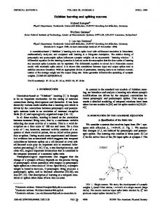
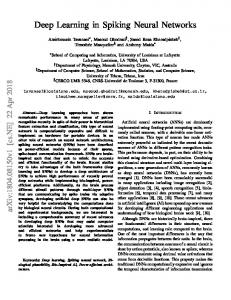
cs ⫺t/␶s, with cf ⫽ ⫺50, cs ⫽ ⫺5, ␶f ⫽ 7 ms, ␶s ⫽ 30 ms, the slow decay with time constant ␶s was added to counteract the influence of the slow response kernel and thus increase the stability during recall, parameter ␤ ⫽ 0.2, learning rate ␩ ⫽ 10, u0 ⫽ ⫺5, and initial model weights zero. Target spike trains were generated by injecting strong external positive currents in high firing rate phases and negative currents in low firing rate phases, which we modeled using neural dynamics given by ui(t) ⫽ u0 ⫹ xi␬ (t) ⫹ uext, where uext ⫽ ⫹50(⫺50) in high (low) firing rate phases of the neuron and the sigmoidal B spiking firing probability. Each high (low) firing rate phase had a duration of 50 ms. The training phase consisted of 3 䡠 10 3 samples drawn from the target distribution. In Figure 5A the change in synaptic strength ⌬w after 50 pairings of one presynaptic with one postsynaptic spike on an interval of 200 ms was computed for different adaption kernels ␬(t) ⫽ ce ⫺t /␶r with ␶r ⫽ 10 ms (black: c ⫽ 2, blue: c ⫽ 0, red: c ⫽ ⫺10) while keeping the synaptic response Figure 1. Task and model description. A, Left, Stimuli-evoked activity patterns v (ticks) with probabilities given by a target 1 ⫺t/␶ ⫺t/␶ distribution P*(v) (curves). Middle, In the absence of stimuli the network spontaneously generates activity patterns x ⫽ (v, h) kernel ␧共t兲 ⫽ ␶ ⫺ ␶ 共e 1 ⫺ e 2兲, with ␶1 ⫽ 1 2 distributed according to a model distribution Pw0 (x) with synaptic strength parameters w0. Right, With learning, the distribution 10 ms and ␶ ⫽ 2 ms. The initial value of the 2 of spontaneous activity patterns Pw(v) approaches the target distribution. Hidden neurons (in gray) help to support the desired membrane potential before stimulation was set activity patterns in the visible neurons. B, Neural dynamics define the model distribution Pw(x) trough a spike response kernel ␧, an to the resting potential u ⫽ ⫺5. Initial weight 0 adaptation kernel ␬, and the spike probability ␳. Minimizing the divergence D(P*(v)储Pw(v)) from the target to the model was w ⫽ 10. In Figure 5B the data were fitted with distribution leads to a plasticity rule for the synaptic strengths w that is matched to the recall dynamics. a model given by the probability function ␳(u) ⫽ g0关u ⫺ ␪兴⫹ 2 ⫹ ␯0, and response kernel ␣共s兲 7 ⫽ ␶␣⫺1exp共⫺s/␶␣兲⌰共s兲 (see above, Link to the weights w0 ⫽ 0, P(x0) ⫽ ␦x0,x*. Training data consisted of 10 patterns of voltage-triplet rule). The fitted parameters are given by the following: g0 ⫽ length 20 time steps, which were generated by the target distribution by 0.94 䡠 10 ⫺2 Hz, ␯0 ⫽ 7.9 Hz, ␪ ⫽ ⫺36.2, ␶␣ ⫽ 41.5 ms, w0 ⫽ 1, and ␩ ⫽ 0.46. running the neural dynamics with target weights w*. The transition fre4 All simulations were performed with Mathematica on personal comquency data was obtained empirically by generating 10 samples of 20 puters, except the simulations in Figure 3, which were written in C and time steps. the fit in Figure 5B, which was performed with MATLAB. Figure 3B shows the same as in Figure 3A but for a different target. The construction of the k ⫽ 3 Markov target is explained in the second paragraph after Equation 6 and in the caption of Figure 3B. We excluded Results target weights w*, which parameterize a distribution with highly correWe studied the task of learning to spontaneously produce lated subsequent visible states, i.e., 具(2vi(t ⫹ 1) ⫺ 1)(2vi(t) ⫺ 1)典t,i,P␪(x) ⬎ spiking activity with a given statistics: stimuli make neurons 0.8, since such distributions can be accurately approximated with a Markovian model. fire in a specific order (Fig. 1A, target); in the absence of any Figure 3C shows the KL divergence after learning for different k. Restimulus, neurons spike spontaneously; and before learning, sults were obtained for 16 different target weight matrices w* and initial the spontaneous activity patterns do not resemble the conditions x*. For simulations with static hidden weights the visible to stimulus-evoked activity patterns (Fig. 1A, before learning). hidden and hidden to hidden weights were the randomly reordered final The goal of learning is to change the network dynamics such that weights from the corresponding simulation with plastic hidden weights, after learning the spontaneous activity patterns resemble the the initial visible weights were set to zero and trained with the same stimulus-evoked activity patterns (Fig. 1A, after learning). To target. derive plasticity rules that solve this learning task, we chose the In Figures 4 and 5 we identify one simulation time step with 1 ms. neural dynamics and minimized with respect to synaptic weights Figure 4A. Number of neurons N ⫽ Nv ⫽ 100, response kernel time a distance measure between stimulus-evoked and spontaneous constants ␶1 ⫽ 10 ms, ␶2 ⫽ 2 ms, adaptation time constant ␶r ⫽ 15 ms, adaptation kernel amplitude c ⫽ ⫺10, parameter ␤ ⫽ 1/3, learning rate activity (see Materials and Methods; Fig. 1B). In this way, the ␩ ⫽ 0.5, resting potential u0 ⫽ ⫺5, initial model weights zero, target learning rule is matched to the neural dynamics. weights w*ij ⫽ 20, if i 僆 {10(l ⫹ 1) ⫹ 1, … 10(l ⫹ 2)} and j 僆 {10l ⫹ 1, … To study the proposed learning rules we first elaborate on 10(l ⫹ 1)}, w*ij ⫽ ⫺5, otherwise. Training data consisted of 10 6 states deterministic target sequences learned with the simplest variant generated by the target distribution by running the neural dynamics with of our model. Deterministic target sequences are of behavioral target weights w*. relevance, since spatiotemporal spike pattern distributions are Figure 4B shows the number of neurons N ⫽ Nv ⫽ 20, response kernel presumably often sharply peaked in the sense that the typical time constants ␶1 ⫽ 10 ms, ␶2 ⫽ 2 ms, adaptation time constant ␶r ⫽ 3 ms, spike patterns closely resemble each other. adaptation kernel amplitude cadapt ⫽ ⫺200, parameter ␤ ⫽ 0.1, learning rate ␩ ⫽ 100, resting potential u0 ⫽ ⫺5, initial model weights zero, delta target distribution P*(x) ⫽ ␦x,x*, with x* drawn from a distribution with P(x*i (t) ⫽ Deterministic target sequences 1) ⫽ 0.1, the learning phase consisted of 2 䡠 10 4 target pattern presentations. In the simplest conceivable form of our model the shape of the For recall, the system is always initialized in the same way. postsynaptic kernel ␧ is a unit rectangular for one delayed time Figure 4C shows the number of neurons N ⫽ Nv ⫽ 10, fast response step and no adaptation takes place. This stochastic McCullochkernel kernel time constants ␶1 ⫽ 15 ms, ␶2 ⫽ 7 ms, slow response kernel Pitts neuron (McCulloch and Pitts, 1943) is of widespread usage time constants ␶1 ⫽ 50 ms, ␶2 ⫽ 30 ms, adaptation kernel ␬(t) ⫽ cf ⫺t/␶f ⫹

A

9570 • J. Neurosci., June 5, 2013 • 33(23):9565–9575

Brea et al. • Sequence Learning

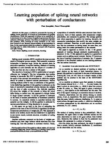
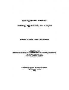
in artificial neural networks (Baum and Wilczek, 1987; Du¨ring et al., 1998; Barber, 2011). In Figure 2A, target, we show a sequence, which is learnable with only visible neurons. During learning, the stimuli activated the neurons repetitively in the order shown in the figure. After learning, spontaneous activity reproduced the target sequence including the transition from the last to the first spatial activity pattern. This fact is also reflected in the learning curve in Figure 2A, which shows that the model distribution approximated the target distribution almost perfectly. Which sequences are learnable with only visible neurons and which require hidden neurons? Since at each moment in time a neuron can be either active or silent, the total number of visible sequences is 2NvT, for a given number of visible neurons Nv and sequence length T. We can group these sequences using as criterion either linear separability or Markovianity (see Materials and Methods). It turns out that this grouping helps to formulate minimal architectural requirements, as summarized in Figure 2C: linearly separable sequences can be learned with only visible neurons and synaptic connections between them, Markovian sequences require enough (at most Nh ⫽ T ) hidden neurons and at least synaptic connections from visible to hidden and hidden to visible, and non-Markovian sequences demand additionally connections between hidden neurons. The sequence shown in Figure 2A is linearly separable and thus can be learned with Figure 2. Learnability of deterministic target sequences with a network of McCulloch-Pitts neurons. A, Linearly separable only visible neurons. The sequence in Figure sequence can be learned with only visible neurons. B, The fraction of learnable sequences with only visible neurons for different 2E is non-Markovian: the state marked relative sequence lengths and number of neurons: in red for a learning rule that finds an optimal solution if the sequence is linearly by a blue triangle occurs twice in the separable, in blue for the asymmetric Hebb rule (see Results) (Nv ⫽ 40, 60, 80, light to dark). The dots indicate the mean, the error sequence. Furthermore, already the sec- bars indicate the SD of the posterior distribution with flat prior. C, For a given number of visible neurons Nv and sequence length T, ond state (red triangle), where all neu- the number of possible deterministic target sequences is 2NvT. These sequences can be classified by either linear separability or rons are silent, renders the sequences Markovianity (see Materials and Methods). Linearly separable sequences can be learned with only visible neurons; nonlinearly not linearly separable. This is a conse- separable but Markovian sequences require sufficient hidden neurons and appropriate synaptic weights from visible to hidden and quence of our choice of coding (1, ac- from hidden to visible neurons, and non-Markovian sequences require additionally connections between hidden neurons. D, The tive; 0, silent) and adaptable parameters simple asymmetric Hebb rule (blue curve; see Results) does often not find weights that allow perfect recall if the pattern is temporally correlated. The fraction of learnable patterns (red curve) decreases only slowly with increasing correlation length ␣. E, (only synaptic weights wij), which we This target sequence is obviously not linearly separable and even non-Markovian: it contains an activity gap in the second time step used to account for biological con- (highlighted with red triangle) and in time steps 5 and 9 (highlighted with blue triangles) the same spatial pattern is followed by straints. This sequence can only be two different patterns in time steps 6 and 10. After training, a network with only visible neurons only recalls the gap faithfully when learned with appropriate recurrent con- initialized with the first time step and only reproduces the states up to the ambiguous transition faithfully when initialized with the nections of the hidden neurons. We third time step just after the gap. Shown in each case is an overlay of 10 recalls. With the batch algorithm in Equation 8 and show that both the batch and the on-line the on-line plasticity rule in Equation 12 the sequence can be learned. The states left of the green line were clamped for recall. With learning rule find appropriate synaptic the on-line rule, the system learned to periodically produce the sequence and no further clamping of initial states was required weights by stochastic gradient descent during recall. on the upper bound F of the divergence show the fraction of learnable sequences as a function of the D from target to model distribution. This bound becomes relative sequence length T/Nv for different Nv. Below a relative tight, i.e., F ⫽ D, toward the end of learning (see Materials sequence length of approximately T/Nv ⬇ 1.5 the probability for and Methods), which is reflected in the diminishing distance the sequence to be linearly separable is very close to 1. The critical between the F and D curves in Figure 2E. value T/Nv ⬇ 1.5 is again a consequence of our choice of coding. What is the typical size of the subset of linearly separable, and thus learnable, sequences for given Nv and T? In Figure 2B we For (1, active; ⫺1, silent) coding we expect the critical relative

Brea et al. • Sequence Learning

J. Neurosci., June 5, 2013 • 33(23):9565–9575 • 9571

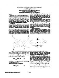
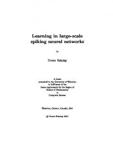
consider correlated patterns (Fig. 2D): the simple temporal Hebb rule performs well only for uncorrelated patterns whereas the probability of linearly separable sequences decreases slowly with increasing correlation. Stochastic target Some stimuli might evoke spike patterns that do not follow a sharply peaked distribution. Instead, the spike patterns look quite different each time a sample from the target distribution P*(x) is drawn. Even though they do not look similar, there might be some temporal dependencies in the sense that the spiking activity x(t) at time t depends on earlier spiking activity states x(t ⫺ k), k ⬎ 0. Variability in the target patterns can arise due to many different reasons. First, there is an extrinsic source of variability, as the same stimulus can be presented with small variations. Second, neurons and synapses are intrinsically noisy, so the neural network that provides the teaching signal will be subject to noise. Interestingly, in the proposed framework the level of noise during recall can be matched to the target variability through synaptic plasticity. As we showed in Materials and Methods (second paragraph after Eq. 6) it is possible to implement a large class of stochastic target distributions, namely factorizable Markov chains product Pw(vi(t) 兩 v(t ⫺ 1), Figure 3. Stochastic targets learned with McCulloch-Pitts dynamics. In all the simulations the target distribution was param- …, v(t ⫺ k)) of order k, which can be parameterized by target weights w*. A, Left, For a Markovian target with only visible neurons (k ⫽ 1) the weights can be learned with a eterized by Pw(vi(t) 兩 v(t ⫺ 1), …, v(t ⫺ k)) model with only visible neurons or a model with visible (1–5) and hidden (6 –20) neurons (upper left submatrix: visible to visible (cf., Eqs. 1 and 2). For Markovian targets connections). Middle, Empirical frequency of subsequent activity patterns v(t) and v(t ⫹ 1). For dots on the black line the model (k ⫽ 1) and a model without hidden neufrequency matches the target frequency. (black, only visible; red, with hidden) Right, The learning curve is similar for both models. rons, the solution is unique due to the conB, A k ⫽ 3 target cannot be accurately learned with only visible neurons but can be learned with a model that includes hidden vexity of the KL divergence. In Figure 3A we neurons. The target was implemented with connectivities such that the first group of hidden neurons (6 –10) receives strong demonstrate in an example that the learning excitatory input from the visible and the second group of hidden neurons (11–15) receives strong excitatory input from the first rule effectively leads to the solution. For group of hidden neurons. The learned hidden weights do not need to be the same as the target weights. C, With increasing complexity (k ⫽ 1 to k ⫽ 4) a model with only visible neurons (black) or static hidden weights (blue) is not sufficient to accurately k ⬎ 1 a model with only visible neurons fails learn the target. The static hidden weights were obtained by reshuffling the weights learned in a simulation with plastic hidden to learn the target, whereas a model with weights. A model with 15 plastic hidden neurons (red) performs well up to the capacity limit k ⫽ 4. Learning stopped after 10 7 sufficient hidden neurons equipped with target samples, even when learning did not converge. Dots indicate the median, error bars indicate the first and third quartile of the our learning rule succeeds (Fig. 3B). Under results from 16 simulations with different targets. the light of the remarkable capabilities of reservoir computing (Maass and Sontag, 2000; Lukos˘evic˘ius and Jaeger, 2009; Rigotti sequence length to be at T/Nv ⬇ 2 (Hertz et al., 1991). As a et al., 2010) it is interesting to note that a random choice of static reference we compare this to a simple temporal Hebb rule hidden weights obtained by reshuffling learned weights is not suffi1 T cient to learn the target (Fig. 3C). ⌬wij ⫽ ⌺t⫽1 共2xi 共t ⫹ 1兲 ⫺ 1兲共2xj 共t兲 ⫺ 1兲 as proposed in T Hopfield (1982); Du¨ring et al. (1998); Grossberg (1969); Herz et ␣-shaped kernels al. (1988); Gerstner et al. (1993); Horn et al. (2000). It is not So far we discussed the plasticity rule for a model with very simple surprising that this simple temporal Hebb rule, for which linear dynamics. However, the neuron model in Equation 1 allows for separability is not a sufficient condition for a pattern to be learnmore realistic dynamics. In the examples shown in Figure 4, a able, in general does not find synaptic weights to perform perfect presynaptic spike evokes an ␣-shaped synaptic response ␧ (Fig. 4B), which is felt by the postsynaptic neuron, and an adaptation recall: instead of solving an optimization problem (minimizing ␬, which prevents immediate follow-up spikes in the presynaptic the divergence from target to model distribution), which leads to cell. With this dynamics it is possible to learn a “synfire chain” a learning rule that is matched to the dynamics, it is simply in(Fig. 4A) or a pattern of precise spike times (Fig. 4B). Depending spired by the symmetric Hebb rule used in Hopfield networks on the target distribution and the neural dynamics, timing errors (Hopfield, 1982). Its weakness becomes even clearer when we

9572 • J. Neurosci., June 5, 2013 • 33(23):9565–9575

Brea et al. • Sequence Learning

may propagate and the pattern eventually becomes unstable (Diesmann et al., 1999). This fading of precision is less problematic with a rate code. In Figure 4C, target, the pattern of Figure 2A is encoded with periods of high and low firing rate. The system can reasonably well learn this target with an ␣-shaped synaptic response ␧1 and adaptation kernel ␬ (Fig. 4C, model with only ␧1, blue learning curve). Fast synaptic responses ␧2 help to further stabilize the pattern and increase performance (Fig. 4C, model with both ␧1 and ␧2, red learning curve). The motivation for using synaptic responses on two different timescales arises from the idea that fast connections establish attractors that encode for the different elements in the sequence and slow responses push the dynamics from one attractor to the next (Sompolinsky and Kanter, 1986). Neurons could implement fast and slow responses to one presynaptic spike with different types of synapses, e.g., fast AMPA synapses and slow NMDA synapses. Biological plausibility When learning is formulated with a computational goal in mind, like minimizing the difference between target and model distribution, it is far from obvious that the resulting learning rule is biologically plausible in the sense that it respects constraints of biological systems and is consistent with experimental data. Here we argue that the proposed learning rule in Equation 12 is biologically plausible. The learning rule in Equation 12 respects causality, is implemented in an online fashion, and depends on presynaptic and postsynaptic x activity and a modula- Figure 4. Target distributions learned with ␣-shaped response kernels. A, The target distribution P*(x) ⫽ Pw*(x) has the tory factor for hidden synapses. The pre- same parametrization as the model with excitatory weights from groups of 10 neurons projecting to subsequent groups of post term shares similarities with STDP: 10 neurons and inhibitory weights otherwise. B, Precisely timed spike patterns can be learned. C, The sequence of Figure 2A Figure 5A shows the STDP window pre- is encoded with periods of high or low firing rate. The target was generated by applying strong input current square pulses. dicted by the learning rule (Bi and Poo, Refractoriness sets an upper bound to the maximal firing rate. In recalls the model system was clamped to the target up to the green line. 1998; Pfister et al., 2006; Brea et al., 2011). Note that this learning rule, which minimodulating factor (see Eq. 12) affects the plasticity of a large mizes the divergence in Equation 3 from target to model, predicts group of synapses (the hidden synapses). Second, according to that the causal part of the STDP window should be matched to our model, this global factor (see Eq. 12) acts at a slower time the dynamics of the synaptic transmission. The acausal part deconstant than the membrane time constant, which is consistent pends on the adaptation properties of the neuron. Interestingly, with the calcium dynamics of astrocytes (Di Castro et al., 2011). the learning rule is closely related to the voltage-triplet rule (PfisFinally, a causal pairing (pre-then-post) can lead either to longter and Gerstner, 2006; Clopath et al., 2010; see Materials and term potentiation or long-term depression depending on the sign Methods) and is compatible with the frequency dependence of of the global factor (r(t) ⫺ r៮(t)). This is in agreement with the STDP as observed by Sjo¨stro¨m et al. (2001) (Fig. 5B). study of Panatier et al. (2006) who showed that when D-serine, For hidden synapses, the plasticity rule does not depend only which is an NMDA co-agonist, is released by astrocytes, longon the presynaptic and postsynaptic activity, but is also moduterm depression can be turned into long-term potentiation. Unlated by a global factor. This global factor could be implemented like what is suggested by Panatier et al. (2006), this type of sliding by astrocytes for mainly three reasons. First, it has been shown threshold (r៮ (t) in our case) is conceptually different from the one that astrocytes, which contact a large number of synapses, can in the BCM learning rule (Bienenstock et al., 1982) since it is a modulate synaptic plasticity (Henneberger et al., 2010; Min and global quantity whereas in the BCM learning rule the sliding Nevian, 2012). Similarly, in our framework, the semi-global

Brea et al. • Sequence Learning

J. Neurosci., June 5, 2013 • 33(23):9565–9575 • 9573

It is interesting to note that the learning rule for the hidden neurons in Equation 12 appears formally similar to a reward-based learning rule (Pfister et al., 2006), but now the reward is an internally computed quantity and does not depend on an external reward. Loosely speaking, if the hidden units contribute to make the visible spikes likely, the synapses targeting those hidden units receive an internal reward signal (r(t) ⫺ r៮(t)) (Eq. 12). The formulation of learning as minimizing the KL divergence (or, equivalently, maximizing the log-likelihood) or an upper bound thereof is common practice in machine learning. The novelty of our approach lies in the specific choice of the upper bound of the KL divergence, Figure 5. The learning rule shares similarities with STDP. A, The STDP window for different adaptation kernels (on the right in which relies on the assumption of condiblack, blue, and red): the synaptic weight change ⌬w of a positive synaptic strength w ⬎ 0 after a pairing protocol on an interval tional independence for the neural firing, of 200 ms, in which both neurons spike once with a separating interval of ⌬t ⫽ tpost ⫺ tpre. Note that the shape of the curve in the i.e., given its membrane potential, the causal part ⌬t ⱖ 0 is determined by the response kernel-shape ␧ and in the acausal part ⌬t ⬍ 0 depends on the adaptation kernel probability of firing of a neuron is condi␬. B, Experimental (black) and model (red) weight change induced by the pairing protocol described by Sjo¨stro¨m et al. (2001). Every 10 s, bursts of five pairs of presynaptic and postsynaptic spike with a relative timing of ⌬t ⫽ tpost ⫺ tpre ⫽ 10 ms (solid lines) tionally independent of the firing of all and ⌬t ⫽ ⫺10 ms (dashed line) are induced at different pairing repetition frequencies. Fifteen such bursts are elicited (which give other neurons at the same time. Even a total of 75 pairs) for all repetition except at 0.1 Hz. At this frequency, only 50 pairs are elicited (Sjo¨stro¨m et al. (2001), their though this assumption is perfectly reaExperimental Procedures). It is assumed that at the beginning of the simulation, the weight is set to 1 and updated only after the sonable and widely used (e.g., in the GLM induction protocol to mimic the time lag between induction and expression in the experiments. framework; Pillow and Latham, 2008), it is the key assumption that allows the joint distribution over visible and hidden activthreshold is a local quantity that depends on the history of the ity to be expressed as a product of a distribution from which it is postsynaptic activity. Note that the proposed global factor deeasy to sample (Qw(h 兩 v)) and a function which is easy to calcupends on activity in visible neurons and affects hidden synapses late (Rw(v 兩 h)). This stands in contrast to temporal Boltzmann only. Thus, if astrocytes are responsible for this signaling, they machines (Sutskever et al., 2009) where this assumption is not “need to know” which neurons are visible and which are hidden. made and sampling usually involves running a Monte Carlo This might be possible due to geometrical arrangement or chemMarkov Chain in each time step, which is hard to justify under the ical signaling. light of biological plausibility. Discussion Another approach to learn a statistical model of spatiotemLearning a statistical model for temporal sequences with hidden poral spike pattern with visible and hidden neurons is a genunits is a challenging machine learning task in itself. Here we eralization of the expectation-maximization algorithm proposed by considered an even harder problem in that we are interested in a Pillow and Latham (2008). Yet, as a version of the Helmholtz biologically plausible learning rule that can solve this task. To be machine, the distribution, from which the hidden states are sambiologically plausible, the learning rule has to be local, causal, and pled, uses a different parameterization for storage (recognition; be consistent with experimental data. We derived a biologically wake phase of learning) and recall (generation; sleep phase of plausible learning rule that minimizes by stochastic gradient delearning) and assumes an acausal kernel, which renders the scent an upper bound of the KL divergence from target to model model unsuitable for a biologically realistic implementation. To distribution. circumvent the need of sampling the hidden states, h ⬃ Pw(h 兩 v) (see Eq. 4), Rezende et al. (2011) proposed to calculate explicitly Because the proposed learning rule is minimizing an upper the expectation under the posterior distribution Pw(h 兩 v). To bound of the KL divergence and not the KL divergence itself and achieve this, they had to assume a weak coupling between neubecause the tightness of the bound is not explicitly controlled, rons and then approximate the true posterior distribution by a unlike in the Helmholtz framework (Dayan et al., 1995), the maxGaussian process on the membrane potential. This weak couima of the two different objective functions could in principle be pling assumption is however difficult to justify at the end of learnlocated at different places in the parameter space. It is, however, ing where individual weights can become large. interesting to note that after some learning time, the bound becomes A drawback of the proposed learning rule for systems intighter, as can be seen on Figure 2E where the KL divergence between cluding hidden neurons is the potentially long learning time. the proposal distribution Qw(h 兩 v) and the posterior distribution Pw(h 兩 v) decreases. In fact, we can show that at the beginning of The plasticity rule relies on stochastic gradient ascent by samlearning and at the end of learning of deterministic patterns, the pling hidden sequences h ⬃ Qw(h 兩 v). As in any gradient descent method, the learning time depends on the learning rate bound is tight. Indeed, at the beginning of the learning all the weights and the initial condition: the learning time is short if at the (and in particular the weights toward visible neurons) are initialized beginning of learning the weights projecting onto hidden neuto zero and therefore, the function Rw(v 兩 h) is independent of the hidden activity and thus D and F are identical. At the end of learnrons are such that the samples h ⬃ Qw(h 兩 v) help to quickly reduce the difference measure between target and model dising, for a deterministic pattern, the proposal distribution is a Dirac tribution and can be long otherwise. In some cases it is even delta distribution and therefore D ⫽ F.

9574 • J. Neurosci., June 5, 2013 • 33(23):9565–9575

possible to find initial weights that supersede any further learning of hidden weights. For example, any possible sequence as discussed in Figure 2C could be learned with a (hardwired) delay line of length T with Nh ⫽ T hidden neurons and no learning of the hidden weights. Alternatively, the delay line could be implemented by a large enough number of randomly connected hidden neurons (Maass and Sontag, 2000; Lukos˘evic˘ius and Jaeger, 2009; Rigotti et al., 2010) where the weights are chosen from a given distribution. The number of randomly connected hidden neurons needed might be very large to guarantee good solutions in any case. Since the goal of this paper was rather to demonstrate that the learning rule is capable of learning distributions that could not be learned with only visible neurons, we did not make use of elaborated choices of the initial conditions and started all simulations with initial weights w0 ⫽ 0. Our paper is not the first one to propose the idea that storage and recall should be matched. Indeed Sommer and Dayan (1998) and Lengyel et al. (2005) already proposed that there should be a tight link between the plasticity rule and the neural dynamics. Interestingly their approach is complementary to the one presented here. Indeed, they start from a given plasticity rule and then derive the optimal (Bayesian) recall dynamics for this given plasticity rule. Here we are following the opposite path. We start from the neural dynamics and then derive the plasticity rule. Given the richness and the accuracy of existing neural models and given the absence of a canonical model of synaptic plasticity, we preferred to start from what is well known and derive predictions on what is largely unknown. An interesting outcome of our model is that the learning rule for hidden synapses does not depend only on the presynaptic and postsynaptic activity, but is also modulated by a global factor. We argued in this paper that this global factor could be provided by astrocytes. To experimentally test this hypothesis we note that the global factor is predicted to depend on the voltage of the visible neurons. In particular, independently of the precise implementation of the model (be it by minimizing an upper bound on the KL divergence as presented here or by directly minimizing KL divergence itself as in Brea et al., 2011), the global factor crucially depends on the presynaptic membrane potential at the time of the spike (see Eq. 10). So the key experimental step would be to show that astrocytic activity depends on the membrane potential of the presynaptic neuron at the time of the spike. This prediction seems plausible since it was found that a depolarization of the presynaptic membrane potential at the time of the spike causes a larger postsynaptic potential (Alle and Geiger, 2006; Shu et al., 2006). We suggest that astrocytes could have a similar sensitivity to the membrane potential at the time of the spike.

References Ackley DH, Hinton GE, Sejnowski TJ (1985) A learning algorithm for Boltzmann machines. Cogn Sci 9:147–169. CrossRef Alle H, Geiger JR (2006) Combined analog and action potential coding in hippocampal mossy fibers. Science 311:1290 –1293. CrossRef Medline Amari SI (1972) Learning patterns and pattern sequences by self-organizing nets of threshold elements. IEEE Trans Comput 21:1197–1206. CrossRef Barber D (2011) Bayesian reasoning and machine learning. New York: Cambridge UP. Barber D, Agakov F (2002) Correlated sequence learning in a network of spiking neurons using maximum likelihood. Tech Report EDI-INF-RR0149, School of Informatics, Edinburgh, UK.

Brea et al. • Sequence Learning Baum EB, Wilczek F (1987) Supervised learning of probability distributions by neural networks. Adv Neural Inf Process Syst 52– 61. Bi GQ, Poo MM (1998) Synaptic modifications in cultured hippocampal neurons: dependence on spike timing, synaptic strength, and postsynaptic cell type. J Neurosci 18:10464 –10472. Medline Bienenstock EL, Cooper LN, Munro PW (1982) Theory for the development of neuron selectivity: orientation specificity and binocular interaction in visual cortex. J Neurosci 2:32– 48. Medline Brea J, Senn W, Pfister JP (2011) Sequence learning with hidden units in spiking neural networks. Adv Neural Inf Process Syst 24:1422– 1430. Clopath C, Bu¨sing L, Vasilaki E, Gerstner W (2010) Connectivity reflects coding: a model of voltage-based STDP with homeostasis. Nat Neurosci 13:344 –352. CrossRef Medline Dayan P, Hinton GE, Neal RM, Zemel RS (1995) The Helmholtz machine. Neural Comput 7:889 –904. CrossRef Medline Di Castro MA, Chuquet J, Liaudet N, Bhaukaurally K, Santello M, Bouvier D, Tiret P, Volterra A (2011) Local Ca2⫹ detection and modulation of synaptic release by astrocytes. Nat Neurosci 14:1276 –1284. CrossRef Medline Diesmann M, Gewaltig MO, Aertsen A (1999) Stable propagation of synchronous spiking in cortical neural networks. Nature 402:529 –533. CrossRef Medline Du¨ring A, Coolen A, Sherrington D (1998) Phase diagram and storage capacity of sequence processing neural networks. J Phys A Math Gen 31: 8607– 8621. CrossRef Elizondo D (2006) The linear separability problem: some testing methods. IEEE Trans Neural Netw 17:330 –344. CrossRef Medline Gerstner W, Kistler WM (2002) Spiking neuron models: single neurons, populations, plasticity. New York: Cambridge UP. Gerstner W, Ritz R, van Hemmen JL (1993) Why spikes? Hebbian learning and retrieval of time-resolved excitation patterns. Biol Cybern 69:503– 515. CrossRef Medline Grossberg S (1969) On the serial learning of lists. Math Biosci 4:201–253. CrossRef Hahnloser RH, Kozhevnikov AA, Fee MS (2002) An ultra-sparse code underlies the generation of neural sequences in a songbird. Nature 419:65–70. CrossRef Medline Henneberger C, Papouin T, Oliet SH, Rusakov DA (2010) Long-term potentiation depends on release of D-serine from astrocytes. Nature 463: 232–236. CrossRef Medline Hertz J, Krogh A, Palmer RG (1991) Introduction to the theory of neural computation. Redwood City, CA: Addison-Wesley Longman. Herz AVM, Sulzer B, Ku¨hn B, Van Hemmen JL (1988) The Hebb rule: representation of static and dynamic objects in neural networks. Europhys Lett 7:663– 669. CrossRef Hinton G, Dayan P, To A, Neal R (1995) The Helmholtz machine through time. ICANN-95 483– 490. Hopfield JJ (1982) Neural networks and physical systems with emergent collective computational abilities. Proc Natl Acad Sci U S A 79:2554 – 2558. CrossRef Medline Horn D, Levy N, Meilijson I, Ruppin E (2000) Distributed synchrony of spiking neurons in a Hebbian cell assembly. Adv Neural Inf Process Syst 12:129 –135. Lengyel M, Kwag J, Paulsen O, Dayan P (2005) Matching storage and recall: hippocampal spike timing-dependent plasticity and phase response curves. Nat Neurosci 8:1677–1683. CrossRef Medline Lukos˘evic˘ius M, Jaeger H (2009) Reservoir computing approaches to recurrent neural network training. Comput Sci Rev 3:127–149. CrossRef Maass W, Markram H (2002) Synapses as dynamic memory buffers. Neural Netw 15:155–161. CrossRef Medline Maass W, Sontag ED (2000) Neural systems as nonlinear filters. Neural Comput 12:1743–1772. CrossRef Medline McCulloch WS, Pitts WH (1943) A logical calculus of the ideas immanent in nervous activity. Bull Math Biophys 5:115–133. CrossRef Min R, Nevian T (2012) Astrocyte signaling controls spike timingdependent depression at neocortical synapses. Nat Neurosci 15:746 – 753. CrossRef Medline Mishchenko Y, Paninski L (2011) Efficient methods for sampling spike trains in networks of coupled neurons. Ann Appl Stat 5:1893–1919. CrossRef Panatier A, Theodosis DT, Mothet JP, Touquet B, Pollegioni L, Poulain DA,

Brea et al. • Sequence Learning Oliet SH (2006) Glia-derived D-serine controls NMDA receptor activity and synaptic memory. Cell 125:775–784. CrossRef Medline Pfister JP, Gerstner W (2006) Triplets of spikes in a model of spike timingdependent plasticity. J Neurosci 26:9673–9682. CrossRef Medline Pfister JP, Toyoizumi T, Barber D, Gerstner W (2006) Optimal spiketiming-dependent plasticity for precise action potential firing in supervised learning. Neural Comput 18:1318 –1348. CrossRef Medline Pillow J, Latham P (2008) Neural characterization in partially observed populations of spiking neurons. Adv Neural Inf Process Syst 20: 1161–1168. Ponulak F, Kasin´ski A (2010) Supervised learning in spiking neural networks with resume: sequence learning, classification, and spike shifting. Neural Comput 22:467–510. CrossRef Medline Rezende DJ, Wierstra D, Gerstner W (2011) Variational learning for recurrent spiking networks. Neural Inf Process Syst 24:136 –144. Rigotti M, Ben Dayan Rubin D, Wang XJ, Fusi S (2010) Internal representation of task rules by recurrent dynamics: the importance of the diversity of neural responses. Front Comput Neurosci 4:24. Medline

J. Neurosci., June 5, 2013 • 33(23):9565–9575 • 9575 Shu Y, Hasenstaub A, Duque A, Yu Y, McCormick DA (2006) Modulation of intracortical synaptic potentials by presynaptic somatic membrane potential. Nature 441:761–765. CrossRef Medline Sjo¨stro¨m PJ, Turrigiano GG, Nelson SB (2001) Rate, timing, and cooperativity jointly determine cortical synaptic plasticity. Neuron 32: 1149 –1164. CrossRef Medline Sommer FT, Dayan P (1998) Bayesian retrieval in associative memories with storage errors. IEEE Trans Neural Netw 9:705–713. CrossRef Medline Sompolinsky H, Kanter I I (1986) Temporal association in asymmetric neural networks. Phys Rev Lett 57:2861–2864. CrossRef Medline Sutskever I, Hinton GE, Taylor G (2009) The recurrent temporal restricted Boltzmann machine. Adv Neural Inf Process Syst 21:1601–1608. Xu S, Jiang W, Dan Y, Poo MM (2012) Activity recall in a visual cortical ensemble. Nat Neurosci 15:449 – 455, S1–S2. CrossRef Medline