Figure 4.22: Normalised PSD of an ML code STDR signal of length 63 chips @ 30MHz (1V ...... http://www.engineering.usu.edu/ece/furse/COE/wiring/Jawss2000.html ...... Instruments, âMeasuring Strain with Strain Gaugesâ, NI Developer Zone,.
LANCASTER UNIVERSITY Centre for Microsystems Engineering Faculty of Applied Sciences Bailrigg Lancaster LA1 3AQ
MEMS Sensors and High Frequency Test Techniques for Prognostic Health Management of Aircraft Wiring Brian Moffat, Marc Desmulliez, Andrew Richardson, Alistair Sutherland.
Table of Contents Chapter 1 Introduction and Report Outline...................................................................... 1 1.1 Introduction............................................................................................................ 1 1.2 Report Objectives................................................................................................... 3 1.3 Organisation of the work........................................................................................ 3 Chapter 2 Failures and causes of failures in avionics wiring........................................... 6 2.1 Wet arcing .............................................................................................................. 8 2.2 Dry arcing .............................................................................................................. 9 2.3 Series arcing........................................................................................................... 9 2.4 Hydrolytic scission............................................................................................... 10 2.5 Mechanical ageing ............................................................................................... 12 2.6 Thermal effects on wiring .................................................................................... 13 2.7 Repeated load and fatigue .................................................................................... 14 2.8 Causes of failure due to maintenance .................................................................. 14 2.9 Intermittency and contact fretting of electrical connectors.................................. 16 2.10 FMEA of aircraft wiring .................................................................................... 19 2.10.4 Summary of FMEA................................................................................... 24 References....................................................................................................................... 28 Chapter 3 Current methods used to detect wire damage................................................ 30 3.1 Discharge phenomena (high potential voltage testing)........................................ 30 3.2 Low frequency and Direct Current (DC) methods............................................... 31 3.3 Tone injection ...................................................................................................... 32 3.4 Smart wire system................................................................................................ 32 3.5 High frequency testing ......................................................................................... 34 3.5.1 Time Domain Reflectometry (TDR)..................................................... 34 3.5.2 Frequency Domain Reflectometry (FDR)............................................. 38 3.5.3 Failures of TDR/FDR............................................................................ 41 References....................................................................................................................... 43 Chapter 4 Spread spectrum technique for wiring fault detection................................... 45 4.1 Spread Spectrum Time Domain Reflectometry (SSTDR)................................... 45 4.1.1 Frequency Hopped Spread Spectrum (FHSS) ............................................. 47 4.1.2 Direct Sequence Spread Spectrum (DSSS).................................................. 48 4.1.3 Sequence Time Division Reflectometry ...................................................... 50 4.2 Fault location in presence of noise....................................................................... 51 4.3 Pseudorandom Codes........................................................................................... 52 4.3.1 Maximum length codes............................................................................... 53 4.3.2 Gold codes................................................................................................... 53 4.3.3 Kansami codes ............................................................................................ 54 4.3.4 Barker codes................................................................................................ 55 4.4 SSTDR/STDR in the presence of white noise ..................................................... 56 4.5 Using SSTDR/STDR in the presence of Mil-Std 1553........................................ 57 4.6 Location of wet and dry arcing ............................................................................ 59 4.7 Conclusion ........................................................................................................... 62 References ...................................................................................................................... 64 ii
Chapter 5 MEMS sensors for location of faults in aircraft wiring................................. 64 5.1 Rogowski coils..................................................................................................... 64 5.1.1 Theory of Rogowski Coil............................................................................. 65 5.1.2 High frequency effects ................................................................................. 66 5.1.3 Fabrication of a micro-engineered Rogowski coil....................................... 67 5.2 Strain gauges ........................................................................................................ 67 5.3 Triboelectric effect............................................................................................... 70 5.4 Conclusion ........................................................................................................... 72 5.4.1 Rogowski Coil ............................................................................................. 72 5.4.2 Strain gauges ................................................................................................ 72 5.4.3 Triboelectric effect....................................................................................... 72 References....................................................................................................................... 74 Chapter 6 MEMS Chemical Sensors ............................................................................. 76 6.1 Humidity Sensors................................................................................................. 76 6.1.1 Dew Point Measurement............................................................................. 77 6.1.2 Surface Acoustic Wave (SAW) Humidity Sensors..................................... 77 6.1.3 MEMS Humidity Sensor Shear/Stress Design ........................................... 79 6.1.4 Thermal Conductivity Humidity Sensors ................................................... 81 6.1.5 Resistive Humidity Sensors ........................................................................ 82 6.1.6 Polymer based relative humidity sensor ..................................................... 84 6.1.7 Capacitive Sensor with porous silicon as the dielectric.............................. 86 6.1.8 Capacitive sensor with dielectric coated electrodes.................................... 88 6.1.9 Interdigitated humidity sensor .................................................................... 89 6.1.10 Wireless capacitive humidity sensors ....................................................... 91 6.2 Corrosion sensors................................................................................................. 94 6.3 Chemical sensor 3 ................................................................................................ 99 6.4 Chemical sensor 4 .............................................................................................. 100 6.5 Conclusion ......................................................................................................... 101 References..................................................................................................................... 102 Chapter 7 Conclusions and future work........................................................................ 105 7.1 Conclusions........................................................................................................ 105 7.2 Future work ........................................................................................................ 109 7.2.1 Time plan ................................................................................................... 109 7.2.2 Set up wire harness test bed for arcing. ..................................................... 110 7.2.3 Further testing on rogowski coil ................................................................ 110 7.2.4 Testing of the strain gauge for wire deterioration...................................... 110 7.2.5 Design and fabrication of humidity sensor ................................................ 111 Appendix A ................................................................................................................... 112 Appendix B ................................................................................................................... 113
iii
List of Figures Figure 1.1: Mil-std 1553 wiring, consisting of databus and LRU’s. ……………...Page 1 Figure 1.2: Outline of research work carried out in this thesis on MEMS sensors and high frequency signal processing techniques for prognostic health management of aircraft wiring. …………………………………………………………………. ...Page 3 Figure 1.3: Chapter Outline……………… ………………….…………………... Page 5 Figure 2.1: Decreases to the wires conductor/insulator thickness over last fifty years. …. ……………………………………………………………………………………..Page 6 Figure 2.2: Bi-directional data transfer in a Line Replaceable Unit………...……..Page 7 Figure 2.3: Typical wire system failure modes 1980-99………………………. …Page 7 Figure 2.4: Carbon track that forms on wiring, lead to a conductive path for current ……. . …………………………………………………………………………......Page 8 Figure 2.5: Low level arcing before flashover. High level arcing during flashover …….. ……………………………………………………………………………………..Page 9 Figure 2.6: Illustration of a damaged bolt head after dry arcing has occurred .. ...Page 12 Figure 2.7: Heat Damage to insulation caused by poor electrical connection (Series Arcing) . ………………………………………………………………………….Page 11 Figure 2.8: Illustration of hydrolytic scission …………………………………....Page 12 Figure 2.9(left): Variation of the breaking strain with molecular weight……..….Page 12 Figure 2.9(right): Variation of the wiring lifetime with humidity and temperature …………………………………………………………………………..………. Page 12 Figure 2.10: How the mechanical stress set up by the electric field causes voids to increase in size ………………………………………………………………... ...Page 14 Figure 2.11: How material approaches fatigue limit with large cycles. ……....…Page 16 Figure 2.12: Asperity interaction due to horizontal motion ……………. ……….Page 18 Figure 2.13: How connector resistance during fretting ……………………...…. Page 20 Figure 2.14: Equivalent circuit of contact impedance ……………………….…..Page 20 Figure 2.15: Taxonomy of failure modes in aircraft wiring (top level) …….. …..Page 21 Figure 2.16: Taxonomy of faults due to mechanical failure……...(Given in Appendix B) Figure 2.17: Taxonomy of faults related to electrical failures …………………...Page 24 iv
Figure 2.18: Taxonomy of faults related to chemical failure modes ………………Page 25 Figure 3.1: The correct test configurations to enable arcing to occur in high voltage testing..…………………………………………………………………………... Page 32 Figure 3.2 Figure 3.3: Aegis Devices Smart Wire System: Three wire fault location method for DC and low frequency measurements …………………………. …...Page 33 Figure 3.4: TDR for open and short circuit terminations …………………… .....Page 37 Figure 3.5: Reflections viewed on TDR for loads comprising complex impedance …………………………………………………………………………………... Page 38 Figure 3.6: Circuit model of a lossy transmission line for two parallel ……………………………………………………………………………………………... Page 38
wires
Figure 3.7: Location of the Dirac Delta Function on Fourier Transform … …….Page 43 Figure 3.8: A transformer coupled test assembly to mimic the layout of Mil-Std 1553 wiring ………………………………………………………………………….... Page 44 Figure 4.1: Overview of MEMS sensors and high frequency testing techniques for fault finding …………………………………………………………………………... Page 48 Figure 4.2: Block diagram of a DSS system and the 3 methods to detect wiring faults …………………………………………………………………………………... Page 52 Figure 4.3: Illustrating how SSTDR locates faults..…………………………….. Page 53 Figure 4.4: The sampling correlator to view the reflections from impedance changes ………….. …………………………………………………………………….....Page 54 Figure 4.5: Various sequences sent down the wire to identify faults using STDR ………………. …………………………………………………………………..Page 54 Figure 4.6: Correlation of received signal in the presence of white noise for SSTDR …………………………………………………………………………………... Page 55 Figure 4.7: Breakdown of the variants of pseudorandom codes …………………Page 56 Figure 4.8: Autocorrelation for ML code ………………………………...……...Page 56 Figure 4.9: Cross correlation of two ML Codes .……………………………...... Page 56 Figure 4.10: Gold Autocorrelation..……………………………………...……….Page 57 Figure 4.11: Gold Code Cross Correlation …………………………………. ......Page 57 Figure 4.12: Kansami code autocorrelation ………………………………..…....Page 57 Figure 4.13: Kansami cross-correlation function …………………………….....Page 57 v
Figure 4.14: Autocorrelation of Barker code …………………………..……. ….Page 58 Figure 4.15: ML code STDR signal @ 1V r.m.s, comprising signal length of 63 chips at 30 MHZ in white noise at 4V r.m.s…... …………………………………… …...Page 59 Figure 4.16: ML code SSTDR signal at 1V r.m.s, comprising signal length of 63 chips at 30MHz, in white noise @ 4Vrms… …………………………………...…...... Page 59 Figure 4.17: Normalised cross correlation of reference ML Code STDR/SSTDR signals … ………………………………………………………………………………...Page 60 Figure 4.18: ML code STDR signal @ 1V r.m.s, comprising signal length of 63 chips at 30 MHz whilst operating on Mil-Std 1553 @10V rms ……………………….....Page 60 Figure 4.19: ML Code SSTDR signal @ 1V r.m.s, comprising signal length of 63 chips @30 MHz, operating on Mil-Std 1553 @10V rms. ……………………………. Page 60 Figure 4.20: Normalised Cross Correlation of a Reference ML Code STDR signal with the signal shown in fig 4.18. ……………………………………………………. Page 61 Figure 4.21: Normalised cross correlation of a reference ML Code SSTDR signal with the signal shown in fig 4.19. ……………………………………………… Page 61 Figure 4.22: Normalised PSD of an ML code STDR signal of length 63 chips @ 30MHz (1V r.m.s), ML code SSTDR signal of length 63 chips at 30MHz (1V r.m.s), and Mil-std 1553 (10V rms). Signals are normalised with respect to the peak STDR Power. ………………………………………………………………………….. Page 61 Figure 4.23: Normalised PSD of the cross correlator output for a pure ML code STDR (ideal case) signal of length 63 chips @ 30 MHz (1V r.m.s) and a 1V r.m.s ML code STDR signal in the presence of a 10V r.m.s Mil-Std 1553 signal. ………………Page 62 Figure 4.24: Normalised PSD of the cross-correlator output for a pure ML code SSTDR (ideal case) signal of length 63 chips @ 30 MHz (1V r.m.s) and a 1V r.m.s ML code SSTDR signal in the presence of a 10V r.m.s Mil-Std 1553 signal... Page 62 Figure 4.25: Wet arc STDR test data with 32.5ft long aircraft cable using 325ft long 75Ω coaxial cable to provide 60Hz 28v AC. A drop of 3% saline solution was dripped over the two nicked wires 25ft from the test system. ………………………....... Page 63 Figure 4.26: Wet arc SSTDR test data with 32.5ft long aircraft cable using 325ft long 75Ω coaxial cable to provide 60Hz 28v AC. A drop of 3% saline solution was dripped over the two nicked wires 25ft from the test system. …………………………... Page 63 Figure 4.27: Dry arc STDR test data with 32.5ft long aircraft cable using 325ft long 75Ω coax cable to provide 60 Hz 28V AC. A 1A fuse was allowed to contact two nicked wires 25ft from the test system. Arc duration was 114ms. …………....... Page 63 Figure 4.28: Dry arc SSTDR test data with 32.5ft long aircraft cable using 325ft long 75Ω coax cable to provide 60 Hz 28V AC. A 1A fuse was allowed to contact two nicked wires 25ft from the test system. Arc duration was 114ms. ………….......Page 64 vi
Figure 5.1: The Rogowski coil and integrator enables measurement of di/dt on a wire ………… ………………………………………………………………………...Page 68 Figure 5.2: High frequency model of Rogowski coil that includes the capacitance, inductance and resistance ………………………………………………………...Page 68 Figure 5.3: Effects of slew rate …………………………………………………..Page 68 Figure 5.4: Passive Integrator ……………………………………………………Page 69 Figure 5.5: A Strain gauge, measuring in the principal direction of deformation ……………………………………………………………………………………Page 70 Figure 5.6: The Triboelectric Effect ……………………………………………..Page 72 Figure 5.7: ABB Group’s new eVM1 circuit breaker, incorporating Rogowski coil and new integrator technology ……………………………………………………… Page 74 Figure 6.1: Illustration between Relative Humidity, dew point and condensation …………. ………………………………………………………………………..Page 78 Figure 6.2: SAW humidity sensor ……………………………………………….Page 80 Figure 6.3: How SAW’s propagate through the sensor ………………………….Page 81 Figure 6.4: MEMS Shear/Stress humidity sensor. Drawing courtesy of Hygrometrix ………. …………………………………………………………………………..Page 82 Figure 6.5: Wheatstone bridge circuit for shear/strain MEMS humidity sensor....Page 83 Figure 6.6: Thermal Conductivity Humidity Sensor …………………………….Page 85 Figure 6.7: Resistive Humidity Sensor…………………………………………...Page 85 Figure 6.8: Selection of resistive humidity sensors ……………………………...Page 85 Figure 6.9: Polymer based Capacitive Relative Humidity Sensor Device …………………………………………………………………………...……….Page 86
Layout
Figure 6.10: How R.H causes a change in capacitance ………………………… Page 87 Figure 6.11: Physical model of polymer based capacitor sensor with top electrode partially exposed………………………………………………….........................Page 88 Figure 6.12: SEM Micrograph of developed Porous Silicon Humidity Sensor …………….. …………………………………………………………………….Page 89 Figure 6.14: Overview of a capacitive sensor with thermoset dielectric coated electrodes ……………………………………………………………………........................Page 91 Figure 6.15: Overview of interdigitated humidity sensors ………………………Page 92 vii
Figure 6.16: Physical and HMS model of the capacitive wireless humidity sensor. ……………………………………………………………………………………Page 94 Figure 6.17: Model of a wireless capacitive humidity sensor and corresponding shift in resonant frequency ……………………………………………………………….Page 94 Figure 6.18: Graph of resonant frequency (MHz) versus relative humidity..........Page 95 Figure 6.19: Graph illustrating frequency dip …………………………...……....Page 96 Figure 6.20: Diagram of electrochemical sensor for detection of heavy metal ions ………………………………………………………………………………......Page 100 Figure 6.21: Principle of how the micro-electrodes operate ……………………Page 101 Figure 6.22: Semtas method of measuring corrosion at the connectors ………..Page 103
viii
List of Tables Table 2.1: Examplar of FMEA for aircraft wiring ……………………………….Page 25 Table 7.1: Timetable for the testing of MEMS Sensors and Spread Spectrum………….. ……………………..............................................................................................Page 111
ix
Chapter 1 Introduction and Report Outline 1.1
Introduction
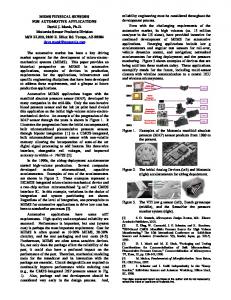
Aircraft wiring technology has evolved over the years due to the introduction to digital systems as a result of advances made in semiconductor fabrication and digital signal processing. These advances led to changes from analog circuitry to the creation of Mil-Std 1553, a digital transmission system and protocol, which enabled systems and subsystems linked into a network to communicate with each other. The system shares the wiring and electrical interconnects with other systems, subsystems and sensors, which enable the devices to share information. The system consists of a number of “black boxes” or Line Replaceable Units (LRUs), which cover a variety of functions ranging from converting signals from one format to another (Remote Terminal), to data monitoring and recording of events such as errors in the system (Bus Monitor), controlling data flow (Bus Controller), or subsystems, and sensors, as figure 1.1 illustrates.
Figure 1.1: Mil-std 1553 wiring, consisting of databus and LRU’s.
Even though systems in an aircraft have been upgraded over the years, the wiring that interconnect them is often neglected. Errors have been reported by either the pilot and/or the system are sometimes undetectable during routine maintenance for two main reasons: either the Automated Test Equipment (ATE) cannot detect the faults until they fail, or the faults only occur during flight. During flight the aircraft wiring is immersed in harsh environments such as vibration, temperature, humidity and corrosive chemical agents. Wiring rubbing against other wiring or structures causes fraying of the insulation and moisture intrusion which leads to the loss of its mechanical and electrical strengths leading to insulation rupturing and leaving the conductor vulnerable to short 1
circuiting with metallic structures and/or other exposed wiring covered in moisture. This form of short circuiting is called “Arcing”, where high energy flashover takes place, which can lead to fire before the circuit breakers can act. Arcing also increases the amount of signal loss and distortion on live signals. This report discusses the detection of a variety of failure modes by utilising MEMS Sensors suitable for in-situ, in-flight testing of the wiring. Of particular importance would be the possibility to diagnose ageing of the wiring before it becomes a safety issue. This research work is carried out in collaboration with BCF Designs Ltd, an English company specialising in wiring test systems and solutions. This company wishes to create a test system to increase levels of safety and confidence and to aid aircraft operators in preventative maintenance, and safety of the wiring, saving thereby on loss of aircraft availability, man-hours and high cost of fault finding. High frequency test techniques such as Spread Spectrum evaluate the suitability for detection of anomalies in the wiring and conditions such as short/open circuits. These techniques perform in the presence of noise and other live data signals that would be present on Mil-std 1553 wiring when the aircraft is in flight and operates fast enough to prevent arcing from manifesting itself into a fire. Whilst the purpose of this thesis is not to research into advanced signal processing methods for fault finding, we will mention nevertheless the current methods used and research whether they can be applied to MEMS. The schematic of the research carried in this report is given in figure 2, which illustrates how MEMS sensors and spread spectrum communication techniques can be linked together to form a prognostics system that not only senses failure in the wiring, by can detect deterioration by sensing the contributing effects that lead to failure.
Aircraft Wiring
MEMS Sensors
High Frequency Testing Techniques
Spread Spectrum Time Domain Reflectometry
Sequence Time Domain Reflectometry
Rogowski Coil
Strain Gauges
2
Chemical Sensors
Humidity Sensors
Figure 1.2: Outline of research work carried out in this thesis on MEMS sensors and high frequency signal processing techniques for prognostic health management of aircraft wiring.
Using spread spectrum techniques enables the location of the fault in the wiring to be found as well as detecting that a fault has occurred. MEMS sensors will enable faults and deterioration in the wire health to be detected. The information obtained by the MEMS sensors and spread spectrum enables the correct decisions to be made concerning the wire health and further opportunities for specific parts of the wiring to fail. This information can be stored in a database with the purpose of scheduling maintenance and further processing to see if more information can be found on the aging affect if the aircraft is operating in a harsher environment than other aircraft.
1.2 Report Objectives The objectives of this project are therefore to: •
Look at the elements of aircraft wiring and perform FMEA (Failure Mode and Effect Analysis) to identify the contributory cause(s) of failure.
•
Identify the contributory effects that lead to failures and review those which are detectable.
•
Review current detection techniques available to test the health of the wiring to see if they can be used in a miniaturised in-situ sensing element that continuously monitors the wire health, without interfering with live signals that would be present during flight.
•
Examine Spread Spectrum techniques to see if it can detect arcing whilst there are live signals present and noise.
•
Prove that such techniques constitute a reliable method able to pinpoint the location of the fault.
•
Analyse available MEMS sensors and techniques that enable new MEMS sensors to be designed that can detect either failure of the wiring and/or detect the deterioration of wiring so that preventative maintenance can be carried out.
1.3
Organisation of the work
In that effect, the plan of the thesis is as follows: •
Chapter 2 gives an overview on the history of aircraft wiring and the issues leading to a variety of failures, as well as an overview of the aircraft wiring system. It then proceeds to describe all types of failure and the resulting effects. Some of the failure effects are more catastrophic than others and in most cases the minor failures lead in time to the aging effect 3
of the wiring and then ultimately catastrophic failure. For this reason Failure Mode Effects and Analysis (FMEA) was performed on the wiring system. This type of analysis breaks down the wiring system down into smaller parts that are considered in terms of possible ways that the part may fail and the consequence of the failure(s). These failures are mapped out to see how they affect the overall system, and how detectable these failures are. •
Chapter 3 evaluates the current methods used to check the wire health starting with DC or low frequency methods, progressing to high potential voltage testing and high frequency testing. Not all of these methods are applicable for the in-situ testing of the wiring and require the wiring harness to be disconnected at a variety of points. However there are methods of non invasive testing such as tone detection that rely on the sensing of magnetic and electric fields, and also the use of current sensors that are used in the Smartwire created by Aegis Devices Inc. that can detect deterioration and faults in the wiring.
•
Chapter 4 moves on to look at more successful high frequency testing methods such as Spread Spectrum Time Domain Reflectometry (SSTDR) and Sequence Time Domain Reflectometry, which are derivatives of Time Domain Reflectometry (TDR), covered in chapter 4. The benefit of this type of sensing is that by choosing the correct signal processing the location of the fault can be detected as well as fault, which cannot be achieved by the MEMS sensors alone.
•
Chapter 5 provides the possible methods of detection using MEMS Sensors. These sensors cover a variety of different detecting mechanisms for aging and failure of wiring starting at the Rogowski Coil, which is a coreless current sensor which has good prospects of detecting arcing and being able to be miniaturised into a MEMS device. The next sensor is a strain gauge which was evaluated for the purpose of detecting the deterioration of the wire by monitoring the changes of strain of the wire. The Triboelectric Effect is discussed also as a method of detecting wire degradation or aging.
•
Chapter 6 presents the final class of the MEMS sensors which is the Chemical Sensor. It predominantly looks at a Corrosion Sensor, with its purpose being that it could be located inside and outside the connector housing. Corrosion plays a large part in the failure of the connectors; therefore being able to detect the onset of corrosion would be of benefit to the system of MEMS sensors being proposed. Other types of chemical sensors have been discussed also for the detection of the aging of aircraft wiring. The final sensor covered in this chapter is a Humidity Sensor, which was chosen for the purpose of monitoring the surrounding environment of the wire and hence the aging effect that occurs in the presence of humidity.
4
Chapter 1 Introduction and Thesis Outline Chapter 2 Types of Wire Failure and FMEA Chapter 3 Existing Methods of Fault Detection Chapter 4 Spread Spectrum Time Domain Reflectometry
Chapter 5 MEMS Strain Gauge and Rogowski Coil Chapter 6 MEMS Humidity Sensor and Chemical Sensors Chapter 7 Summary Chapter 8 Further Work
Figure 1.3: Chapter Outline
5
Chapter 2 Failures and causes of failures in avionics wiring Over the last fifty years there have been changes to the wire insulation in terms of size and weight in order to keep the weight of the aircraft down. Figure 2.1 illustrates how the size of the conductor and the insulation of the wire have decreased to meet tighter demands from aircraft designers. At present the thickness of the insulation can be approximated to the width of three human hairs, as shown in Figure 2.1.
Figure 2.1: Decreases to the wires conductor/insulator thickness over last fifty years. Dimensions in inches [2.26].
A report by Blemel et al [2.1] at the 2000 Aging Aircraft Conference highlighted that at present the B52 aircraft has seen its lifetime extended for up to four times than it was designed for. It is reckoned that the B52 will last at least 60 years more than its original life expectancy. For many years wiring in avionics was overlooked as being a prominent cause of system failure in comparison to other electrical sources on board of an aircraft due to the intensive man hours and cost required to rewire the plane [2.2-2.6]. Faults with aircraft wiring were originally attributed to Line Replaceable Units (LRU’s), with cases reported that many LRU’s were reported faulty and often replaced without careful consideration as to the state of the wiring connecting these LRU’s or “Black Boxes”. The function of the Line Replaceable Unit is illustrated in figure 2.2. It was designed to enable aircraft wiring to be upgraded from purely analog communication where information was transferred serially, to an array of complex electronics, which enabled bi-directional data communication with the other systems and subsystems.
6
Figure 2.2: Bi-directional data transfer in a Line Replaceable Unit.
It has been claimed that two out of three LRU’s that had supposedly failed were not in fact faulty [2.1]. Even when maintenance was being carried out by trained personnel, there were still errors in the wiring that was not being brought to their attention. Loose connections and prominent cracks, frays and heat damaged areas of wiring were being identified in most cases. There were, however, situations where frays were too small to the human eye to be identified or not easily detectable especially in some planes where the wiring extends for up to 350 kilometres.
Figure 2.3: Typical wire system failure modes 1980-9 [2.26],
Wiring issues usually result in extended loss of usage time and aborted flights. To make things worse, these anomalies can present themselves during flight whilst remaining undetectable during routine maintenance. A possible example is in fuel management systems. A disastrous wiring problem in July 17th 1996, where the Trans World Airlines flight exploded, was due to an arc in the fuel tank. These systems are designed to take into account that the fuel tanks are located in hard to reach areas, and the tanks themselves are not uniform in dimensions, since they are constructed to fit within the wings of the aircraft. Possible sensors to detect the level of fuel are arrays of capacitive probes, which when summed, determine the amount of fuel onboard by the total capacitance of the probes. These probes are often embedded to an extent within the fuel tank,
7
therefore testing the connections and the condition of the wiring and the probes is hard as well as recognising the condition of the probes themselves.
2.1
Wet arcing
Wet arcing occurs in the presence of moisture or fluids on board an aircraft where leakage currents run on the insulation layer of a wire due to small cracks or voids. This causes a heating effect of the moistened insulation, drying it out and leaving it with a dry band or spot being formed as shown in Figure 2.4. These spots present a high resistance to currents and a voltage drop. The energy dissipated leads to small surface discharges being emitted with temperatures of around 1000˚ C easily attainable. It has been claimed by Blemel et al that the insulation will degrade to form carbide crystals at the effected area and on contact with water will release a highly flammable gas that will ignite on ignition of the arc [2.1].
Figure 2.4: Carbon track that forms on wiring, lead to a conductive path for current [2.8].
The seriousness of this type of arcing is emphasised in Kapton, a polyimide used for insulation. This is an aromatic insulating polymer (compounds with carbon ring structures such as benzene), which becomes conductive at high temperatures [2.2-2.8]. Its manufacturer, DuPont, claims that Kapton is resistant to fire, and research suggests that, when the insulation is subject to arcing, it will burn fiercely due to changes in its material structure at temperatures around 1000˚ C, [2.2-2.5].
Figure 2.5: Low level arcing before flashover. High level arcing during flashover [2.8].
These temperatures occur due to the aromatic structure of the polymer, where, as stated earlier, the pyrolysis of the polymer leads to the formation of a carbon track, which, due to its graphitic lattice structure, is very conductive [2.7-2.8]. At the next discharge there will be an explosive flashover 8
that will propagate through the carbon tracking and onto other wire bundles. Due to the current that flows through the track being on the outside of the insulation rather than the centre conductor of the wire, the circuit breakers are unlikely to trip, leaving the arc to sustain itself further down the wire or bundle across to other areas of wiring. As the arc grows there is less chance of it being detected by the circuit breaker due to the current becoming less than what is required by the circuit breaker. In instances where the circuit breaker does trip, stopping extreme damage being done to the bundle, it has been reported that, due to pilots resetting the breaker, the arcing has immediately started and propagated through bundles causing fires in part of the aircraft.
2.2
Dry arcing
Insulators like Kapton that possess the carbon-ring structure also arc without the presence of moisture, where total destruction of a wire bundle has been witnessed [2.2], [2.7] due to a wire with broken insulation touching another wire at another potential of a part of the aircraft structure.
Figure 2.6: Illustration of a damaged bolt head after dry arcing has occurred [9].
In a NASA report on arcing, on inspection of a bolt-head involved with dry arcing, there was an area where metal ejection has occurred due to the sputtering effect of the arc as shown in figure 2.6. This was attributed to paint having been removed with time from the bolt-head, leaving it as an exposed conductor instead of the insulated painted surface which should have been present [2.9].
2.3
Series arcing
Series arcing begins with corrosion in pin-socket connections or loose connections in series with electrical loads. The voltage drop inside a loose connector begins at a few hundred milli-volts and slowly heats or pyrolizes the surrounding media [2.7, 2.8]. After this stage the voltage increases to a few volts, where a glowing connection is most probable and smoke is emitted from the surrounding insulation. This may present itself in the cabin as flickering lights.
9
Figure 2.7: Heat Damage to insulation caused by poor electrical connection (Series Arcing) [2.8].
The current in this instance is limited by the impedance of the electrical load that is connected to the circuit, where the power is also far less than for the parallel case [2.8]. The detection of this type of arcing is far more difficult than for parallel arcing due to the fact that the signature of the arc is the unusual signature of the normal load current. The dangerous part of this type of arcing is that the current remains below the limit that will trip the circuit breaker. The symptoms associated in this case are load voltage drops, heating of the wire, pin and sockets, which results in the failure of the component and source of ignition.
2.4
Hydrolytic scission
The process of hydrolytic scission is a dominant process in the degradation of the wiring insulation due to the molecular structure of the polymer that renders it vulnerable to moisture absorption Kapton, an aromatic polyimide, was the primary insulating material used in MIL-W-81381 wire. The polymer was originally chosen for its good dielectric and mechanical strength at high temperatures. However, reports suggest [2.10, 2.11, 2.13-2.15] that this type of wiring is not as immune from the effects of harsh environment as initially thought. The Kapton insulation has a repeating chain of one dianhydride and one diamine. The ideal polymer chain is a stable repeating unit. There are imperfections in the real polymer chain, which react with water that is absorbed in the polymer chain from high humidity exposure. This results in the chain being broken down into smaller chains, hence having a lower molecular weight [2.8, 2.10-2.15].
10
Figure 2.8: Illustration of hydrolytic scission. [9].
The above figure describes this process, where the original chain is seen (step 1), the water reacts with the imperfections in the chain (step 2), the chain has now been fractured into smaller ones (step 3).
Figure 2.9(left): Variation of the breaking strain with molecular weight. [12, 14, 15]. Figure 2.9(right): Variation of the wiring lifetime with humidity and temperature [12, 14, 15].
The result of this reaction is that the molecular weight of this polymer is reduced, as in figure 2.9, rendering it more brittle and decreasing thereby the lifetime of the wire. It is this reduction in molecular weight that is one of the primary reasons for the degradation of the insulation. The rate of degradation of the insulation is temperature dependant.
11
2.5
Mechanical ageing
Mechanical failure is primarily caused by the electric field set up in the wire creating a tensile mechanical strain at the electrode-dielectric interface. The Lippmann electro-chemical equation states, that a change in potential difference, ∆V, across an interface, causes a change of interfacial tension, ∆γ, according to the relation [2.14, 2.15]: ∆γ = -q∆V .,.…………………………………………………………….....Equation 2.1 where q is the charge separation across the interface. When considering the actual balance between the electrical and mechanical forces present in the interface it is possible to write [2.13 13]: δ
∆γ ≈ − ∫ εE 2 dz ……………………………………………………...………Equation 2.2 0
This equation defines how the electric field, E, normal to the interface of thickness δ, creates a change in the transverse mechanical tension which acts to expand the interface against the cohesive forces that set up ∆γ. When E is large enough and there are voids or micro cracks then the tensile mechanical stress set up by this field may be large enough to cause the void to stretch further, propagating through the wire as shown in Figure 2.10.
Figure 2.10: How the mechanical stress set up by the electric field causes voids to increase in size [2.14].
The propagation occurs by the breaking of the bonds of the dielectric in the path of the fracture of the crack, where energy is released by the change in the stress caused by the bonds breaking causing the crack being driven forward. The other way in which Kapton insulation degrades mechanically has been talked about in section 2.4, where the reaction of the insulation layer with water and water vapour leads to the polymer chain being shortened [2.10-2.12]. The polymer chain of the insulator decreases to such an extent 12
that the strain due to the insulation being wrapped and bent in a position equals the actual breaking strain. When this condition occurs, the insulation will rupture spontaneously, exposing it to the harsh environment surrounding it and leaving it vulnerable to future arcing events [2.2]. The mechanical strain becomes significant in wiring failure modes in two other ways: 1.
With the wire in a bent position and therefore strained, the strain impacts a molecular level energy that decreases the effective activation energy of the defective weaker sites of the polymer with water. Therefore, wiring in bent positions will therefore age at a far quicker rate than wiring in its normal straight position due to its losing its original physical characteristics. The greater the bend of the wire, the higher the molecular energy created by the strain and hence the quicker the ageing process. This also explains why there are specified maintenance guidelines as to the maximum bend radius that wiring should have around the aircraft.
2.
The rupturing of the insulation depends on the amount of strain within the insulation at the moment of rupture. If the wiring is left to age without additional bending strain being impacted on it then it will last longer till a point such that it is moved or flexed by maintenance engineers, causing it to rupture.
2.6
Thermal effects on wiring
Fluctuations in temperature cause thermal stresses within a material in all directions. For most structural materials, the thermal strain, εT, is proportional to the temperature change, ∆T, through the coefficient of thermal expansion (CTE), α [2.16]: εT = α ∆T ………………………………………………………………..…Equation 2.3 Note that the CTE usually depends also of the absolute temperature. If the material is homogenous and isotropic, the increase in any dimension is found by multiplying the original dimension by the thermal strain, [2.15]: δL= εT * L = α.∆T.L. ……………………………………………………...Equation 2.4 Wiring has layers of different materials with different thermal properties and hence different thermal expansion coefficients. If the conductor inside the wiring expands at a greater rate that the insulator then interfacial tension between the layers and cracks appear [2.15]. Wide temperature variations lead to the eventual hardening of the material into a more brittle state, where the application of stress above the minimum breakdown strength causes the insulation to crack. Many 13
areas of wiring within an aircraft are in state where they would fail below the maximum stress stated by the manufacturer.
2.7
Repeated load and fatigue
A structure that is modelled or structured in a dynamic load will subsequently fail at a lower stress than if the load were a statistical one, especially in cases with large number of cycles [2.16].
Figure 2.11: How material approaches fatigue limit with large cycles.
Failure is caused by progressive fracture or fatigue, whereby fatigue is given as the deterioration of a material under repeated cycles of stress and strain resulting in the formation a fracture. In normal fatigued failure, a microscopic crack forms at the point of high stress, which increases in size as the loads are repeated. This effect can be found in wiring that is in a bent position or stressed state, where, if there is a large amount of vibration or impact on this wiring then the aging process of the wiring is accelerated to point of failure far earlier. It is therefore intuitive to try and monitor vibration levels throughout the wiring and the interconnections. As the interconnections begin to fail, they become relaxed and therefore do not maintain as much force to enable a full electrical contact. This causes poor electrical connections to be made and leads to problems such as contact fretting and/or series arcing phenomena to occur.
2.8
Causes of failure due to maintenance
Failures due to maintenance are not the dominant cause of failure as shown in Figure 2.3, though a thorough understanding of the failures of that type is required to avoid any damage to the wiring. Harnesses need to be well routed and supported in the correct manner to ensure that the wire does not flex or vibrate against other wiring or parts of the aircraft structure. This precaution is due to the straight line memory of wiring such as Kapton making it to flex back to its originally unstrained position. Not all wiring is constructed of Kapton, and some is not as strong and hard as Kapton which can abrade, chafe and eventually cut through the insulation of softer insulation types. By 14
twisting the wiring (one to two turns per foot), the harness keeps more flexibility by allowing the wiring to bend through rotational motion rather than it being stressed by the stretching that occurs. During maintenance, technicians should always make sure that when the connectors are being removed that supports are installed to ensure no additional stress is placed on the rest of the wiring and connectors. When wiring is to be bent to curve round bends, the radii of the curve should not exceed the stated amount. The bend should be very slight as excessive bending of the wire to turn round a corner will cause the insulation to crack. When new wiring is installed, care should be taken to ensure that it is not fixed in a stressed state by the length of wire being too short. An ample length should be chosen to ensure it can flex slightly, hence avoiding additionally stress on the wire and connector. Wiring looms should never be stood on to reach harder areas for inspection as this creates additional unplanned stress on the wiring that could cause it to fail. In some cases when wiring can be inspected there can be failed areas that cannot be noticed due to the small size of the flaw.
15
2.9
Intermittency and contact fretting of electrical connectors
Intermittency is a vastly unsolved problem in electronics in terms of adequately detecting it in the early stages and being able to differentiate from it and the case of no faults being found [2.17]. A large amount of ATE equipment in the market place claim to be able to detect it with existing digital testing methods, only for users to find that they have re-named the no fault found result (NFF) with another ambiguous acronym. The issue with intermittency is that existing digital methods only sample for a certain period in time [2.17] or are able to detect the fault once it has manifested itself in its final failure mode as a hard fault. Intermittency has a variety of contributing mechanisms from vibration to temperature gradients. If the boundary of the connector interface is considered at the micro-scale, it becomes more apparent what the problem is.
Figure 2.12: Asperity interaction due to horizontal motion [2.18].
As the two contacts move relative to one another, the micro-protrusions that make up the surface will contact each other at specific points. Micro-protrusions are the highest peaks on the surface of the connector, and when they collide, they will resist further motion till a force of certain magnitude will cause a shearing force that will break of these protrusions as loose particles [2.18]. Vibration levels in aircraft are dominant enough for it to have detrimental effect on the lifetime on the connectors that join various nodes of the wiring. The other form of deterioration that occurs at the connector surface is adhesion, which is when there are high stress concentrations at certain points such as micro-protrusions. This causes micro welding of certain contacting points of the connector surfaces, which will remain welded till a sufficient force is applied to break them.
16
Due to only a small portion of the original contact area actually making contact, electrical continuity relies on these points on the surface actually continually making contact. Processes such as oxidation, thermal expansion, galvanic corrosion and fretting serve to degrade the contact area and increase the contact resistance [2.19]. Both these modes of failure present themselves electrically as random changes in resistance as the contacting surfaces change relative to one another, and as the condition worsens, the faults will become more pronounced over background noise. Work by Mano et al [2.20, 2.21] prove that the environment can get in between the contacting micro-protrusions due to corrosion beginning at he ends of the contacts and stopping them from making full contact and therefore allow corrosion to enter further into the contacts. This has the effect of corroding the whole contact area and cutting off the supply of current. Further research in this paper suggest also that for failure to occur would take up to 300 years at 25ºC and 3 years at 125ºC, and that these figures could be even less due to the nonlinearities no accounted for in the model in his research. Other explanations for contact fretting include the corrosive particles generated on the connector electrode boundaries being dragged into the shallow areas of the conductor surface and at 20nm would stop electron tunnelling from occurring, hence stopping current flow [2.22]. These explanations serve to explain why there are transient changes in the connector resistance over its operating lifetime, and why normal ATE equipment cannot detect it until it is just before the connector actually fails, as figure 2.13 shows. When the environment that aircraft wiring is immersed in is considered, especially the high thermal gradients, humidity changes and corrosive elements such as chlorine and hydrogen, then it becomes justified to link fretting issues within the FMEA of wiring. Bare metal contacts subjected to high amounts of vibration still have the ability to fail due to fretting corrosion by increase in the contact resistance. When enough wear of the conductor surfaces has occurred, there will again be removal of particles and the formation still of abrasive oxides, which serves to increase the rate of wear. At low vibrational frequencies fewer cycles are required for an increase in the contact resistance. Micro-protrusions are vulnerable to corrosive attack for much longer periods for it to manifest itself into greater corrosive thicknesses between movements between the contacting surfaces.
17
Figure 2.13: How connector resistance during fretting [2.22].
Baisheng et al has shown that fretting resistance should be modelled as an impedance when considering high data rate transmission rather than a DC resistance [2.23]. His work looks at the effects that this has on unmatched circuits, rather than the ideal case. The ideal case is that the wires are electrically lossless and that the source and load impedance equal the characteristic impedance of the cables, as described in chapters 2 and 3. The lossless case is where the impedances that make up the system such as the cables and connectors not being equal in impedance and as a result multiple reflections occur at all points in the circuit where there are impedance changes. This case is most approximate to real systems, and it is seen that fretting resistance increases the error rate in data transmission systems. Figure 2.14 depicts the circuit model for fretting resistance for the high frequency case.
Figure 2.14: Equivalent circuit of contact impedance [2.23].
As mentioned prior, the contact area (Ab) is mad up of a number of spots where actual electrical contact is made, and is of a much smaller area of contact. These spots allow the flow of current, and due to the spots being so small cause an increase in resistance, aptly named the constriction resistance. Since these spots are smaller than the non conducting area of the contact area and the distance between conducting spots being small, the parasitic capacitance at high frequencies becomes dominant. In the situation where contaminants have entered between the conducting
18
surfaces at thicknesses of around 20nm as mentioned earlier, then upon full separation the contact approximates a capacitor. Ultimately, this leads to higher rates of error code in digital transmission and in the instance of contact failure at both ends of a cable in an unmatched circuit, the reflection of the signals will become more complex.
2.10 FMEA of aircraft wiring Failure Mode and Effect Analysis (FMEA) is defined [2.24, 2.25] as “the method of effectively breaking a system down into various subsystems and elements so that they can be considered individually on the probability of failure, and how the individual failures contribute to failure of the subsystem and whole system”. There may be more than one cause or contributor of failure, and these are again considered individually so that further redesign can be conducted with the objective of reducing system failure. It is a preventative analytical technique that has employed for around 40 years, where it was initially used in the 1960s for the aerospace industry, for preventive safety measures.
The rationale for using this method in this chapter is to establish the prevalent
contributors to avionics wire failure.
Wiring Failure Modes
Mechanical Failure
Electrical Failure
Chemical Failure
Figure 2.15: Taxonomy of failure modes in aircraft wiring (top level).
For complex systems it may necessary to break the subsystems down into more manageable parts so that full consideration is given and a proper FMEA is conducted, thereby identifying all possible modes of failure, malfunction, or premature aging. The key question in an FMEA is how and why a system can fail, and what problem does this present to all the other manageable parts of the system. In this research the system has been broken down into the elements that make up the aircraft wiring and then considered in terms of electrical, mechanical and chemical failure modes. The steps taken are as follows:
19
Step 1: Break down the electronics into the wiring and interconnect. Step 2: Consider the chemical, electrical and mechanical forms of failure. Focus on one subsystem or manageable subsection to ensure that all effects of failure are found. Step 3: List the effects of each failure mode. There are specially designed FMEA sheets for performing this analysis so that each failure mode and these effects are listed. Sometimes there is only one effect, other times there are multiple. This is the reason that the system should be broken down into manageable sections to ensure full analysis is performed. Step 4: Assign a severity rating, where available to each effect of the failure mode. Step 5: Assign an occurrence rating for each failure mode. Step 6: Assign a detection rating for each failure mode and/or effect. For steps 4-6, the rating are given on a scale from 1 to 10, with 1 being lowest and 10 being the highest. The severity rating is how serious the effects would be if failure occurred. Due to each failure maybe possessing a number of effects of different severity, it is the effects that are judged and not the failure. The assignment of an occurrence rating is obtained from testing the failure or consulting relevant available data in the concerned area. In the case of no data being available, an estimate is given based on available knowledge of the failure. This has been provided by work done by Phillips and is provided in Appendix B. The detection rating is based on the chance that failure or the effect of it can be detected. Step 7: Calculate the risk priority number for each failure effect. This number is calculated as follows: Risk Priority Number (RPN) = Severity multiplied by Occurrence multiplied by Detection. All the calculated RPNs are added for so that the original system can be compared to the upgraded system to see how much it is improved by and if further work can/should be done to increase reliability and functionality of the system. A spreadsheet is given in the Appendix B which was derived by research carried out by Phillips. The spreadsheet denotes a framework for assigning values for occurrence, where the greater the chance of occurrence the lower the number. For high probability of occurrence, values such as 0.33 were used, whereas for low probability values such as 1.67 were used. Step 8: Prioritise the failure modes in terms of importance. These will be failures and/or effects of highest severity. 20
Step 9: Consider means of eliminating failure or detecting it before the failure modes becomes fatal to the subsystem or system.
2.10.1 FMEA of mechanical failures The FMEA of mechanical failures is provided on a separate sheet in landscape format.
Figure 2.16: Taxonomy of faults due to mechanical failure (Given in Appendix B)
The FMEA as applied to mechanical failures is presented in Figure 13. Although the actual failure mode of the wire rupturing is not excessively dangerous when the aircraft is on the ground, it becomes far more serious when the aircraft is in flight. In this instance, there will be electrical power present and varying conditions in terms of humidity, temperature, pressure and vibration. These conditions accelerate the conditions required for serious failure to occur due to arcing and/or loss of signal transmission on the Mil-Std 1553 data bus system that is present on aircraft. What is of interest is the level of maintenance induced errors that contribute to the failure modes. Clamping wires in tight positions and excessive bending lead to chaffing or the degradation in physical properties of the wire as per section 1.5 and 1.8, leading to the formation of larger cracks. This is a failure mode in itself, which with the addition of varying environmental conditions within the aircraft cause it to escalate to a level of catastrophic consequences. The other modes of failure in the maintenance subsection could, with hindsight, be avoided with correct training procedures and therefore serve to increase the chances of the wire not failing too early. The subsections on vibration and temperature are characteristic of the ageing process of wiring and cannot be avoided in most cases. Possible cases of excessive vibration/strain in the wiring as well as the temperature cycling should therefore be tracked. Changes in the material hardness/strain should also be monitored as indicators of the amount of ageing, stress and amount of time till the wiring approaches a state where failure is imminent.
2.10.2 FMEA of electrical failures Failure by electrical means is by far the most dangerous and catastrophic failure mode in wiring. Electrical ageing of the insulator exists due to the fact that it carries current and hence to an extent 21
heats up the wiring. Electrical arcing occurs not only as an electrical failure mode but as a final contributor to all other failure modes. This report aims to research this failure mode, by using MEMS sensors and/or high frequency testing methods to enable the state of the wiring to be determined and appropriate action taken to replace the wiring before it approaches a state where arcing will occur. The connectors have been deemed in various reports to be the cause of fires also, with section 2.3 outlining how contact resistance at the connector pins can increase to such an extent that it can heat up the surrounding connector and wiring to point of fire and hence failure. Electrical Degradation Of Wiring
Connectors
Insulation
Fuel Probes
Environmental changes
Alternating E-Fields
Connection to probe oxidises
Moisture degrades seal
Contact Fretting
Interfacial stresses at insulator/ conductor interface
Poor connection
Series arc tracking
Intermittency
Small cracks created and increase in length along crack
Incorrect probe reading
Loss of data transmission
Dry arc tracking
Wet arc tracking
Loss of subsystem functionality
Figure 2.17: Taxonomy of faults related to electrical failures
Data transmission can still be lost even in the event of no fire, which can have just as catastrophic effects on safety with the potential loss of control of the aircraft. This failure mode is often characterised by rapid changes in electrical impedance of the wire, though it is also worth considering methods of embedding sensors within a connector to detect the state of the surrounding environment in terms of temperature and gases present.
2.10.3 FMEA of chemical failure modes The FMEA related to chemical failure illustrates how it is one of the primary causes for the ageing of the wiring. Chemical reactions have a cumulative effect that manifests itself to a point of failure during arcing and/or the loss of signals transmission occurs on the data bus.
22
Chemical Degradation of Wiring
Humidity Variations
Oxidation of Connector Contacts
Moisture deposited on wiring
Increase in contact resistance
Hydrolytic Scission of insulation
Wet arc tracking
Reduced molecular weight of insulation Loss of Electrical Strength of dielectric
Loss of Mechanical Strength
Electrical Loading
Excessive mechanical loading
Breakdown of Insulation
Insulation cracks
Localised heating of material
Connectors and insulation heat to point of fire
Figure 2.15: Taxonomy of faults related to chemical failure modes
This FMEA shows a starting point for the electrical degradation of the wiring and the connectors that make up a majority of the electrical system. The degradation exists as outlined in section 2.4, with moisture or moisture vapour accelerating the ageing process to a point where either a mechanical cause contributes to the ageing process or the reaction with the insulation with water occurs at such a rate that the physical characteristics of the wiring is degraded. This results in cracks beginning to appear in the wiring, where the presence of moisture and live signals on the wiring will be sufficient for arcing to occur. This is also the case with the connectors, where once the seal has degraded and/or the connector has been disconnected for sufficient time, then oxidation of the contacts will begin, resulting in changes to contact resistance. There have also been reported instances as per section 2.4, where the connectors have been inadequately reinstalled leading to arcing occurring between the connector pins. As a consequence of this FMEA it is desirable to be able to monitor the humidity levels throughout all areas where the aircraft wiring is immersed, in order to establish if there is greater probability that the concerned areas will incur a more rapid change in ageing characteristics.
23
2.10.4 Summary of FMEA An example of a table concerning aircraft wiring is given below in table 2.1. The FMEA highlights that wiring can fail from a wide range of contributory environmental effects. Whilst one cause of failure can start the accelerated ageing of the wiring (i.e. hydrolytic scission), it can ultimately be another source of failure that causes the wiring to catastrophically fail, i.e. bending the wire past the specified bend radii causing the insulation to crack and eventually cause an arcing event. Device: Aircraft Wiring
Prepared by: B. Moffat, M. Desmulliez
24
Effects of Failure
25
Local Effect Effec t on unit
Occurrence
Causes of Failure
Severity
Potential Failure Mode
Detect
Item/ Function
RPN
Insulation
Interfacial Tension
A.C E-Field
Voids/ Cracks
2
Lowering of mechanical strength of insulation
Exceeding Max bend radii/wire in strained position/ vibration Large variations in temp
Voids/ cracks
2-7
Cracks appear/ insulation will crack on next mech. Loading
2-7
Moisture
Decrease in molecular weight/
Moisture/ cracks/ dry tracks on insulation Exposed conductor touches aircraft or other wires Corrosion in pin socket/ loose connection in series with load Vibration induced movement of conductor interface
Fatigue
Hydrolytic scission Wet Arc Tracking
Dry Arc Tracking
Connector
Series arc tracking
Contact Fretting
Aging effect/ Insulation cracks
Aging/ Failure
7
0.67
9.38
Aging/ Early failure
7
0.33
4.62 16.2
Material becomes stiffer/ages
Aging/ Early failure
4
0.83
6.64 – 23.2
7
Loss of material strength
cracks appear early
8
0.33
18.4 8
flashover /Carbon deposits/fire
710
Burnt insulation, Which carbonises, allowing higher energy arcing/fire
Loss of aircraft control/ fire
10
0.67
46.9 -67
flashover /Carbon deposits/fire
7
Burnt insulation, Which carbonises, allowing higher energy arcing/fire
Loss of aircraft control/ fire
10
0.67
46.9 1
Flashover, i2R heating of surrounding area, pyrolysis
5-9
Burnt/smouldering insulation, smoke, loss of signal transmission
Loss of aircraft control/ fire
10
0.83
41.5 74.7
Corrosion, increase in contact resistance, loss of electrical contact
3-7
Loss of signal transmission, series arc tracking
Loss of aircraft control and/or fire
7
0.51
10.5 -25
Table 2.1: Examplar of FMEA for aircraft wiring Note: The numbers used in this analysis were rough guesses and will be supported with experimental evidence when it becomes available.
To be able to detect the wire ageing, or failure of wiring and its location, the FMEA will be consulted and the contributing factors to these failure modes need to be evaluated to see if there is possible MEMS sensor designs that can be coupled with advanced signal processing techniques such as spread spectrum reflectometry techniques to be able to detect arcing, open circuits and short circuits. The MEMS sensors will be evaluated to see if there are methods of detecting if the wiring has aged past the limit where it would not pass the safety and criticality test. The primary effect of the ageing effect of the wiring is that it loses its mechanical and electrical strength. This is attributed to the large fluctuations in temperature and humidity, resulting in the moisture being absorbed into the wiring and breaking up the polymer chain of the insulation into smaller parts, leaving it prone to cracking due to the temperature fluctuations aiding the drying out effect of the insulation. This in turn causes the material to make a transition into a more brittle state. 26
From this understanding it is desirable to be able to monitor areas where there are large fluctuations in humidity. Humidity sensors are evaluated later in this report with regard to incorporating them in the inside and outside of the wire connectors. They will be able to monitor the environment that the wiring is in when placed on the outside of the connector, while inside the connector they will be able to detect if moisture is actually penetrating the connector seal and leading to oxidising on the conductor pins and/or arcing. Mechanically, the insulation can be degraded by excessive fatigue, i.e. vibration, or by a sudden mechanical load. This could be technicians standing on wire bundles to reach often inaccessible areas of wiring. Failure will tend to occur in areas where the wire is bent, hence decreasing the strength of the insulation far quicker than areas where the wire is left in a straightened position. It will be of interest to consider the application of strain gauges for monitoring the varying levels of vibration of the wire as well as measuring the change in axial to transverse strain to see if there is correlation in a change of Poisson’s ratio to the ageing or hardness of the insulation. FMEA has shown that chemical and mechanical strains exacerbate the ageing process by the decomposition of the material characteristics, yet extreme failure such as fire or fire induced damage of other wiring or structures derive from electrical origins. When an aircraft is in flight the electrical systems are in operation and hence the problems are present. Once current is flowing within the system, failure modes present themselves by arcing and/or loss of signal transmission, hence leading to fire and/or loss of control of the aircraft. Faults of this nature are characterised by the change in electrical characteristics such as reflections of signals of impedance discontinuities such as open or short circuits. When arcing occurs it can be characterised as a short circuit momentarily for a few milli-seconds and is hence detectable, as shown in chapter 3 and 4.
27
References [2.1] Kenneth G.Blemel and Peter A. Blemel, Management Sciences Inc., “Smart Wiring Prognostic Health Management” JAWSSS 2000, May 13th. http://www.engineering.usu.edu/ece/furse/COE/wiring/Jawss2000.html [2.2] [12] F. Dricot and H.J. Reher, “Survey of Arc Tracking on Aerospace Cables and Wires”,IEEE Trans. on Dielectrics and Electrical Insulation, Vol. No. 5, October 1994. [2.3] “Aircraft Electrical Wire Types associated with Aircraft Electrical Fires, An aviation safety article, by Alex Paterson, http://www.vision.net.au/~apaterson/aviaton/wire_types.htm [2.4] MD-11 Corrective Action Plan: A Case Study in Reactive Safety, Air Safety Week, Dec 13th 2004. [2.5] “Kapton, A Dangerous Aircraft Wiring Product implicated in Aircraft Electrical Fires” posted online by Alex Paterson. http://www.vision.net.au/~apaterson/aviation/kapton_mangold.htm [2.6] Aviation Today, Column: Avionics System Design-How Parts and Systems Age, by Walter Shawlee. [2.7] “The RAF Experience with Aromatic Polyimide http://www.iasa.co.au/folders/Safety_Issues/Aircraft_Wire/RAFKapton.html
Aircraft
Wiring”,
[2.8] T. Potter, M. Lavado, C. Pellon, Texas Instruments, “Methods of Characterising Arc Fault Signatures in Aerospace Applications”, 2003 Aging Aircraft Conference [2.9] Steven J. Daniels, National Aeronautics and Space Administration (NASA), “Space Shuttle Columbia Aging Wiring Failure Analysis”, 2005 Aging Aircraft Conference, Florida. [2.10] A.M. Bruning and F.J. Campbell, “Aging of Wire Under Multifactor Stress”, IEEE Trans. on Elec. Insulation, Vol. 28, No. 5, Oct. 1993. [2.11] F.J. Campbell and A.M. Bruning, “Insulation Aging from Simultaneous Mechanical Strain, Polymer-Chemical and Temperature Interactions”, 1992 Conf. on Electrical Insulation, Baltimore, USA June 7-10. [2.12] F.J. Campbell, Naval Research Lab, Washington, “Hydrolytic Deterioration of Poilyimide Insulation on Naval Aircraft” [2.13] Christopher Teal and William Frequency”.
Larsen, “The Phenemology of Wire, Dielectrics and
[2.14] P. Connor, J.P. Jones, J.P. Llewellyn and T.J. Lewis, “A Mechanical Origin for Electrical Aging and Breakdown in Polymeric Insulation”, 1998 IEEE Int. Conf. on Breakdown in Solid Dielectrics, June 22-25, Sweeden.
28
[2.15] T.J. Lewsi, J.P. Llewellyn, M.J. van der Sluijs, J. Freestone and R.N. Hampton, Univ. of Wales, 7th Conf. on Dielectric Materials Measurements and Applications, 23-26 September, 1996., “A New Model for Electrical Aging and Breakdown in Dielectrics”. http://www.aviationtoday.com/cgi/av/show_mag.cgi?pub=av&mon=1100&file=column [2.16] Gere and Timoshenko, “Mechanics of Materials” 4th Edition, PWS Publishing Company. [2.17] Universal Synaptics, “Intermittence and its labels”. http://www.usynaptics.com/intermit.htm. [2.18] Dr. James Moran, Dr Matthew Sweetland and Prof. Nam P. Suh, “Low Friction and Wear on Non Lubricated Connector Contact Surfaces”. [2.19] Michael D. Bryant, Dept. of Mech.Eng., University of Texas, “Resistance Buildup in Electrical Connectors due to Fretting Corrosion of Rough Surfaces”. [2.20] E.Takano and K. Mano, “Theoretical Lifetime of Static Contacts”, IEEE Trans. on Parts, Materials and Packaging, vol. 4, pp. 184-185, 1967. [2.21] E. Takano and K. Mano, “The Failure Mode and Lifetime of Static Contacts,”IEEE Trans. on Parts, Materials and Packaging, vol. 4, pp. 51-55, 1968. [2.22] Michael D. Bryant, dept. of Mech. Eng, University of Texas. “Assessment of Fretting Failure Models of Electrical Connectors” [2.23] Baisheng Sun, Lab of Testing Technology and Automation Apparatus, Beijing University of Posts and telecommunications, China. “Effects of Electric Contact Failure on Signal Transmission in Unmatched Circuits” [2.24] Shrikanth Lavu, “1st Year Report in FMEA of MEMS Micromotor”, Heriot-Watt University, 2004. [2.25] BS 5760-5:1991, “Guide to Failure Modes, Effects and Criticality Analysis (FMEA and FMECA)”. [2.26] A Risk Analysis of a Wire Failure Potential in the Aircraft Industry, Aging Aircraft Conf 2005] [Air Safety Week, Vol. 18, No. 20
29
Chapter 3 Current methods used to detect wire damage 3.1
Discharge phenomena (high potential voltage testing)
High testing voltages are commonly used to test damage in aircraft wiring harnesses. However, for optimum detection, the amplitude of the voltage must be high so that flashover at the failure point in the wiring can be observed, [3.1, 3.2]. This type of testing method can lead to damage to voltage sensitive components inside the aircraft. High voltage testing is however only possible in configurations where a flash over can take place between a fault in the wire and a counter electrode as shown in Figure 3.1.
Figure 3.1: The correct test configurations to enable arcing to occur in high voltage testing [3.1].
Paschen’s law governs the minimum breakdown voltage, Vd, necessary for a flashover to occur between two electrodes at a separation d [3.1]. Such a voltage depends on the material and gap between the electrodes separation. By replacing the atmosphere that the wiring is immersed in by an inert gas such as helium or argon, the detection of the wiring fault can be detected at a smaller magnitude of breakdown voltage. This method is called Gas Discharge Method. However, this method does not lend itself well to testing of faults while there are still live signals on the wire, for example. whilst the aircraft is still in flight since the high voltage will corrupt the transmitted data on the wire and cause malfunctions of the aircraft systems.
30
3.2
Low frequency and Direct Current (DC) methods
The application of a current across suspected faulty wires whilst the voltage is measured between these wires is one of the most common methods to measure wiring defects. If a short circuit is detected, then by measuring the resistance between both ends of the wires the percentage of wire on each end of the short circuit can be established. Once the wire diameter is known, the percentage of the cable on each end of the wire can be converted to the distance to the fault location. This method is best suited to low resistance short circuits since, for high resistivity wires, small inaccuracies in percentages can lead to large inaccuracies in the distance to fault location. The other option is to apply a current to two of the conductors which are short circuited together [3.3]. If the current is seen to flow across one of the wires a resistive divider network is created with a tap at the location of the short circuit. If conversely, no current flows across the short circuit then the voltage on the second wire is equal to the voltage on the first wire. The figure below illustrates this, with V2 and V4 measured with respect to ground as i3 is negligible.
Figure 3.2: Three wire fault location method for DC and low frequency measurements
The fault location can be obtained by calculating the ratio of voltage on each side of the fault. For example: V1 ≈ V3 ≈ V2
R1 ……………………………………………………….Equation 3.1 R1 + R2
And
31
L1 ≈ LT
V1 − V0 …………………………………………………...…….....Equation 3.2 V 2 − V0
Where LT is the total length of the wire. This fault location method works for establishing low and high resistance short circuits. Again, this method has the same shortcomings as in the Gas Discharge Method in that it is unsuitable for testing live wires due to the corruption of the transmitted data by the test signals. All areas of wiring cannot also be submitted to this method since a portion of the wiring systems are located in inaccessible areas.
3.3
Tone injection
In this method, a voltage or current is sent down the wire to be tested and a technician walks along the section of wiring with an electric or magnetic field sensing probe. The wire radiates a magnetic and electric field around it when signals are being sent down it, which the probe will pick up. If there is a cut or fray in the wire then it will change the electric field pattern due to the change in uniformity of the insulation, and the probe a tone on identification of a field. If the fault is a short circuit then the probe will make a tone up until the location of the short circuit. If the fault is insulation damage, then a high voltage is applied to the wire under test and an arc is created, which in turn causes a short circuit and the probe will stop making the audible tone when it reaches the arc [3.3, 3.4]. For testing an open circuit, a voltage is applied across the wire to be tested, and an electric field probe is moved along the wire, producing an audible tone till the open circuit is found. These methods are more suited for testing of wiring in homes rather than aircraft due to the aircraft wiring possessing shield areas, and electric/magnetic field being unable to show up where the shielded areas are. Currents or voltages would have to be applied to the wires if the aircraft was not in flight, and disconnection of the wiring harness would have to be undertaken. The probe could check the wiring if there were live signals present, but it is not possible for a technician to be able to check every wire continuously whilst in flight, and some areas are inaccessible in the aircraft for the technician to access.
3.4
Smart wire system
Aegis Devices Inc. has developed a smart wire system that enables the inspection of wire harnesses without being disconnected. This results in real time wire health monitoring [3.5] without 32
interfering with live data present on the wires. This type of sensor has significance to this research as it is a method of fault detection that this research is to investigate, and serves as proof that it is a feasible method of detecting faults. Chapter 5 evaluates the Rogowski Coil for this application, as well as possible other methods of obtaining information on wire health. The system consists of modules that monitor the signals within the aircraft wiring, and summarises and stores the information for future reference. The main part of the system that enables detection of faults is the Hall Effect current sensor, with split core design, which can detect AC and DC signals. The split core design enables these current sensors to be installed without disconnecting the wire harness.
Figure 3.3: Aegis Devices Smart Wire System
The Hall Effect sensor has its output signal conditioned by converting the magnitude of the measured current into a certain value which is proportional to the actual strength of the signal being measured. It is then converted to a digital signal before being sent to the multiplexer. Depending on the value received, it will issue a digital message representing the values of current measured, which is then forwarded on to the Bus Unit. This unit receives the information of the current sensors at specified intervals which can be set according to the aircraft wiring system. The specified intervals are set by the Smart-pro part of the system, such as: •
every few microseconds.
•
When the smartpro requests this information.
•
When the digital message changes, for example if it detects a fault.
After the information has been processed a message is prepared and sent over the CAN Network to the Smart-pro. The CAN Network is an ISO 11898 Controller Area Network, which was chosen due its low power consumption and ease of integration. There is a logic unit that dictates how the power is used from the CAN network so that various modules can be powered for certain sensors, for example areas of wiring that are vulnerable to failure. 33
The Smart-pro can communicate with the smart wire system(s), the display and a database which records information on all areas of the wiring, including scheduling maintenance for connectors at point of failure. The system can handle hundreds of current sensors on the same CAN network, and if necessary for larger groups of wiring can be extended to include multiple Smart-pros to enable all parts of the wiring to be tested continuously. When the connectors have first been installed in the wiring, this company have designed a Smart Mapping Tool to enable all connectors to be mapped out in relation to the wiring bundles. This tool is hand held and is connected to the connector the first time it is installed, where it is assigned an ID number, enabling the mapping to be carried out. Once this is done, the information is passed on to the Smartpro. The final system also uses Time Domain Reflectometry for diagnostics whilst the aircraft is not operational. There is the capability that this system can be connected to the web for aircraft technicians to perform further diagnostics. The structure of this type of sensor presents an idea of the system hierarchy of the current sensor for development in this research. The idea of being able to map out the connectors from using a unique ID enables an accurate idea of the branched wire network that exists within the aircraft, and the way that the information can be stored, processed and accessed in flight could enable the aircraft technicians to develop a more accurate and robust testing methodology that prevents failure and aircraft down time. Further integration of other MEMS Sensors into a connector that uses current sensors should enable a host of environmental factors into account to predict the onset of wiring degradation.
3.5
High frequency testing
High frequency testing uses reflectometry techniques to measure changes in line impedance. Depending on the type of wire being tested, the exact location of the wire anomaly can also be found. The two main techniques are defined as Time Domain Reflectometry (TDR) and Frequency Domain Reflectometry (FDR), [3.3, 3.6-3.16].
3.5.1 Time Domain Reflectometry (TDR)
34
TDR works on the principle that, when a step voltage signal is sent down in a transmission line of characteristic impedance, Z0, a portion of the signal is reflected at a discontinuity in the impedance.
Figure 3.4: TDR for open and short circuit terminations [22]. In order to grasp the idea behind TDR, the behaviour of a wire carrying high frequency signals must first be understood. These effects on wiring and the derivation of the characteristic impedance of the wire are based on the lossy circuit model as given in Figure 3.3. The characteristic impedance is defined as the ratio of voltage to current at every point along the line and determines the amount of current flow when a voltage is applied to an infinitely long line. It also describes discontinuities in the wiring as changes in the impedance along the line from the characteristic impedance will cause reflections to occur [3.3]. The time taken for a signal to travel down and reflect back from an anomaly in the wire contains information on the distance to the fault, whereas the magnitude of the reflection itself describes the type of fault [3.3, 3.6-3.10]. The magnitude of the reflection is governed by the reflection coefficient, ГL, given by: ΓL ≈
ZL − Z0 …,………………………………………………...……..…..Equation 3.3 Z L + Z0
where ZL is the load impedance. Γ is equal 1 for an open circuit and -1 for a short circuit as per Figure 3.4. At an open circuit there is an abrupt increase in the characteristic impedance, whilst a short circuit denotes a decrease in Z0. Complex loads will be characterised by a complex value between these two limits [3.6]. Examples of complex impedance viewed on TDR are given below in Figure 3.5:
35
Figure 3.5: Reflections viewed on TDR for loads comprising complex impedance [3.6].
Figure 3.6: Circuit model of a lossy transmission line for two parallel wires [3.3].
The figure shows the behaviour of two current carrying parallel wires. Four components: resistance, conductance, capacitance and inductance are used to characterise electrically the system at certain frequencies and conditions. When a voltage is applied across two wires, an electric field is created. As the resulting current flows down the wires a magnetic field is induced. These fields interact with surrounding materials including the insulation and nearby structures, wires, etc. The series resistance, R, represents the series resistance of the wire in terms of ohms per unit length. This resistance increases if there is corrosion present in the wire or the wire diameter decreases due to crushing or stretching [3.3]. It decreases if the wire conductivity increases (thicker wire gauge, use of more conductive metals, etc). Since any dielectric, even air, is not a perfect insulator then a small current called “leakage current” will flow between the two wires. In this case, the insulation acts like a resistor connected between the two wires, which permit the flow of current through between these wires. This conductance, G, expressed as micro-ohms per unit length, is large if there is an electrical path between the wires, i.e. if there is water present between the wires, arcing etc. The series inductance, L, is a function of the diameter and profile of the wire, and changes as the wires come into proximity to metal or other materials that interact with the magnetic field around
36
the wires. When a wire changes its permeability to a higher value then its local inductance increases above its nominal value. The shunt capacitance, C, is a function of the wire shape, separation and the permittivity of the intervening materials. In most cases this is a function of the type of insulation used, the separation of the wires and the thickness of the insulation. The shunt capacitance decreases as the wires are separated and also as the insulation is rubbed of. Consider the distance between the wires to be smaller than the wavelength of interest. In this configuration the fields around the wires are transverse to the direction of propagation (TEM mode), i.e. the electrical field vector goes from wire to wire and is perpendicular (transverse) to the wire. The magnetic field is around the wires (ortho-radial direction) and negligible along the wires.
−
∂i ∂v ≈ ri + l ………………………………………………….……..…...Equation 3.4 ∂z ∂t
−
∂v ∂i ≈ gv + c ……………………………………………………...….....Equation 3.5 ∂z ∂t
The equations above govern the behaviour of voltage and current along two wire transmission media for an incremental change in distance, δz, along the wires. For wires in good condition, the conductance and the resistance can be approximated as zero. Therefore equations 3.4 and 3.5 can be expressed as: −
∂i ∂v ≈ l ………………………………………………………….............Equation 3.6 ∂z ∂t
−
∂v ∂i …………………………………………………………….......Equation 3.7 ≈c ∂t ∂z
Differentiating these two equations with respect to z and t, respectively and then combining them yields the following relation: u≈
1 lc
……………………………………………………………….……Equation 3.8
where v( z , t ) ≈ v + ( z − ut ) + v − ( z + ut ) …………….……………….….........Equation 3.9
i( z, t ) ≈ i + ( z − ut ) − i − ( z + ut ) ……………………………………...…….Equation 3.10
37
Equation 3.8 denotes the Velocity Of Propagation, VOP, of the wire, which permits to calculate the location of the wire anomaly from the signal that is reflected. If this velocity is inaccurate, the location of the fault will be erroneous, [3.3, 3.7, 3.8]. The velocity u, ranges from 0.5 to 1 time the speed of light. The signal takes time τ ≈
L to travel down the full wire. Wires in good condition u
generally behave as set out by equations 3.9 and 3.10. VOP poses problems for twisted pair wiring due to it not being constant along the wire length. This has the effect of causing the higher frequencies to be transmitted at much slower speeds compared to lower frequencies. This is known as dispersion. Further rearrangement of the previous equations leads to the definition of Z0: 1 v+ ≈ ≈ + cu i
l v− ≈ Z o ≈ − ………………………………...……...……….Equation 3.11 c i
Z0 increases when the inductance becomes more dominant, and decreases if the capacitance dominates. To determine the distance to the wiring fault, l and c must be constant with distance otherwise problems emerge. The only way to enable constant impedance is through using controlled impedance wiring such as twisted pairs or shielded wires. In the case of bundled wiring such as in avionics wiring, the impedance is not constant along the length which leads to errors when estimating the distance to a defect in the wiring. Frays in wire insulation only in the presence of air are quite difficult to detect and can be attributed to the presence of noise in the TDR or wire dwarfing [3.9]. However, if the fray is grounded to some part of the aircraft or has moisture present then the impedance change becomes far more prominent. When moisture is present the impedance displays the characteristics of a temporary short circuit and the TDR response highlights a greater difference. The disadvantages about TDR is that the electronics are expensive and complex compared to FDR, however performing Fast Fourier Transform on the data obtained in FDR enables TDR data to be obtained and vice versa.
3.5.2 Frequency Domain Reflectometry (FDR) In FDR the phase of the reflected waveform is examined rather than the time taken for the signal to reflect back, [3.3, 3.7, 3.13-3.16]. A sinusoid test signal is sent down the wire and the time delay causes a phase difference to the reflected waveform. If the signal encounters an open or short circuit in the wiring then an abrupt phase change will occur. The phase change provides information on the length and nature of the anomaly on the wire. For this to successfully occur without phase wrapping the length of the wire under test is smaller than the wavelength of the sine wave. Compared to TDR, FDR uses far simpler and smaller electronics, with the required sinusoidal frequencies being
38
generated by a simple VCO. Knowing the optimum performance for TDR determines the optimum performance for FDR, where the optimum pulse width for the TDR results in the optimum sweep frequency range for FDR operation. A greater response to frays could be seen if an FDR Analysis was done in the lower frequency range which would show a greater response in terms of amplitude of the reflection from the fray [3.9]. Another interesting result from [3.9] is the production of small sinusoids where arcing or fraying occurs after a Fast Fourier Transform (FFT) of the baseline measurement has been performed. Brent Waddoups work supports these findings also in [3.8]. He found that the detection of cable frays was indeed frequency dependant and that the optimum frequency range for detection was 200-400MHz, for fray lengths of around 1cm that penetrate all insulation layers and/or shielding layers to the actual conductor. FDR uses a range of stepped frequencies rather than just one frequency when ambiguity due to phase wrapping could occur due to multiples of the observed signal being seen plus the change in phase, i.e. L = 3λ+∆λ, rather than just ∆λ. Therefore it is desirable to somehow filter out the measured mλ part of the signal, [3.7,3.13-3.16]. FDR operates by feeding back the reflected signal with the original signal into a balanced mixer. The mixer multiplies the incident and reflected sine waves, resulting in a DC signal being produced at the output. If the original signal is given by Ae-jkL and the reflected signal by BejkL, (-j denotes the 1800 phase change), the mixer gives an output that is the squared magnitude of the voltage:
Vdc ≈ Ae − jkL + Be jkL
2
≈ A 2 e − jkL + ρe jkL
2
≈ A 2 + B 2 + 2 AB cos(2kL) …..Equation 3.12
where ρ is the reflection coefficient given by ρ = B/A and k = 2πf/u, f is the sweep frequency and u is the VOP. The equation contains a DC offset term, A2+B2, as well as the sinusoidal component, 2ABcos(2kL). For longer lengths of cable there is a greater amount of cycles, and the number of cycles or frequency (2kL) of this waveform is proportional to the distance being measured, l, of the cable. The phase of this waveform is also dependant on the termination as well as the cable length. Performing a Fourier Transform on this waveform with respect to the frequency will give a Dirac Delta Function as the figure 3.7 illustrates.
39
Figure 3.7: Location of the Dirac Delta Function on Fourier Transform
The distance of the Dirac Delta Function from the origin is proportional to the distance being measured. The location is a value of 2kL, with k = (2πf)/vp. As with TDR, the travel time for one cycle of the sinusoidal wave to propagate down a length of wire and back to the TDR is given by:
T≈
1 f BW
≈
2L …………………………………………………………….Equation 3.13 u
where fBW is the bandwidth = fSTOP - fSTART. Open circuits and short circuits can be found easily with FDR, [3.3, 3.7, 3.13-3.16]. In instances where the fault is complex, the reflection coefficient for the fault compared to the characteristic impedance can be found from:
ρ≈
Measured _ value _ of _ spectrum _ at _ peak ……………….….......Equation 3.14 2A
The constant 2A is determined by measuring the reflection for an open or short for the wire under test. As mentioned earlier, the number of cycles in the mixer output waveform is longer for longer length cables. This waveform will determine in effect the maximum and minimum cable that can be tested. From the knowledge of Lmax and Lmin, it is possible to find the accuracy of the system (∆L). The accuracy is limited by the Nyquist criterion, which states that a signal should be sampled at least twice the rate as the frequency to enable faithful reproduction. Two data points should therefore be sampled per cycle of the sinusoidal waveform. The minimum length where a fault can be found is given as: Lmin ≈
VOP ………………………………………………………....…....Equation 3.15 2 f BW 40
where 2fBW is the available bandwidth of frequencies that can be generated by the VCO. The maximum length where a fault can be represented without aliasing is: LMAX ≈
VOP ………………………………………………………...…….Equation 3.16 4∆f
The length resolution of this fault measurement system is defined as: ∆L ≈
VOP ……………………………………………….…………...Equation 3.17 2 N FFT ∆f
where NFFT is the number of points in the FFT. With a smaller frequency step size a larger length can be measured, but results in less accuracy in the fault location.
3.5.3 Failures of TDR/FDR TDR tests have been undertaken by BCF Designs Ltd and RAF Brize Norton [3.11, 3.12] to find its limitations on the Mil-Std 1553 databus, a wiring system that is present on all military and commercial aircraft. Although TDR and FDR are suited to testing specific unconnected cabling, it was found not suitable for testing branched aircraft wiring (Mil-Std 1553). The reason for this is that shown with the aid of figure 3.8:
Figure 3.8: A transformer coupled test assembly to mimic the layout of Mil-Std 1553 wiring, [26].
Although TDR can test for discontinuities on the main part of the main bus (i.e. from each end of the 77Ω terminators) it cannot detect crossover, which is when signals from other wires are electromagnetically coupled to the wire under test. For real time monitoring of the system, the wiring would need to be disconnected for the measurements to be made. The stubs in the system connect the Line Replaceable Units (LRU’s) or “Black boxes” to the main databus line. The stubs are connected by either capacitive or transformer coupling, with capacitive coupling being used for
41
shorter stub to main bus connections and the transformer coupling used for longer distances between the stub and main bus. When the TDR is connected at the stub, it cannot see through the transformer coupler, as it only shows an open circuit on the TDR regardless of the condition. A real open circuit would not be differentiated. It cannot detect the condition of other stubs from the stub it is connected to. Finally, when the TDR is connected across the main bus, it cannot see past any of the couplers linking the stubs. Other issues include: •
The difficulty to differentiate between closely spaced stubs.
•
The detection of short to screen.
•
The insertion loss between stub ends.
•
The detection of a transformer or isolation resistance.
In addition to these problems, there is also the case to consider where the Mil-Std-1553 network has multiple branches in it. This results in multiple reflections from all the branch points. This causes spurious information being obtained due to the multiple reflections superimposing on the TDR pulse, making it harder to tell if the reflection on the TDR is from a fault or from a reflection of a junction further ahead in the wiring, remembering that whatever signal sent will have been attenuated as it travels along the wire and back. The other issue to taken into account for this type of fault detection is the inability of these systems to detect faults in the presence of other signals without distorting them, like the case of Mil-Std-1553 signals. For this reason, FDR and TDR will not be used directly to find faults on aircraft wiring when there are live signals present. Chapter 4 presents a topology for analysing the wire health and detecting faults.
42
References [3.1] Josef Hanson, WEE Electrotest Engineering GmbH, Hafenstrasse, Germany, “Testing Methods for Detection of Insulation Damage in Aerospace Wiring Harness”. [3.2] Dr Josef Hanson and Mathias Spies, “Testing and Assessment of Electrical Systems in Aging Aircraft”, 6th Joint FAA/DoD/NASA Aging Aircraft Conference-Sept. 16-19 2002. [3.3] Paul Smith, “Spread Spectrum Time Domain Reflectometry” 2004 PhD, Utah State University. [3.4] J.B. Hudson, “Facilities Engineering- Electrical Exterior Facilities”. http://www.usace.army.mil/inet/usace-docs/armytm/tm5-684/index.htm Nov. 1986 [3.5] Erik C. Carlson and Chris Ellis, Aegis Devices Ltd., “A Smart Wire System for Non Destructive Inspection of Aircraft Wire Harnesses”, 6th Joint FAA/DoD/NASA Conference on Aging Aircraft, San Fransisco, CA, USA, Sept. 16-19, 2002. [3.6] Agilent High Precision Time Domain Reflectometry Application Note 1304-7 [3.7] Rakesh Dangol, Dr Cynthia Furse, “Use of Frequency Domain Reflectometry for Calculating Length and Load Impedance of Cables” Masters Thesis, Utah State University, 2000. [3.8] Brent Waddoups, “Analysis of Reflectometry for Detection of Chaffed Aircraft Wiring Insulation”, Masters Thesis, 2001, Utah State University. [3.9] Brent D Waddoups, Dr Cynthia Furse and Mark Schmidt,. “Analysis of Reflectometry for Detection of Chafed Aircraft Wiring Insulation”, Fift Joint NASA/FAA/DoD Conference on Aging Aircraft 2001. [3.10] Mark Schmidt, “Practical mtesting of Aircraft Wiring and Insulation Faults”, Masters Thesis, 2002, Utah State University. [3.11] BCF Designs, “Fault Finding in Mil-Std-1553 Databus” [3.12] B. Evans, BCF Designs Ltd., RAF Brize Norton, “Evaluation of a TDR to Fault Find on a Mil-Std-1553 Databus”. [3.13] Arvind Jayakar, “Use of Frequency Domain Reflectometry for Analysis of Cable Trees”, 2001 Masters Thesis, Utah State University. [3.14] Jeremy Pruitt, “Simulation and Analysis of Four Navy Aircraft Wiring Harnesses using Frequency Domain Reflectometry”, Masters Thesis, 2003, Utah State University. [3.15] Santi Bhushana Reddy Basava, Cynthia Furse, “Signal Processing Solutions to Detect and Locate Cable Faults in Aging Aircraft Wiring Using Reflectometry Methods”, 2003 Masters Thesis, Utah University. [3.16] Krishna Konda, “Hardware Connectivity for Live Wires”, Masters Thesis, 2003, Utah State University. 43
44
Chapter 4 Spread spectrum technique for wiring fault detection This chapter explains a methodology for solving the issues aforementioned in chapters 2 and 3. The figure below illustrates the various MEMS sensors and high frequency techniques that will be utilised to detect faults and ageing in aircraft wiring.
Aircraft Wiring
High Frequency Testing techniques
Spread Spectrum Time Domain Reflectometry
Sequence Time Domain Reflectometry
MEMS Sensors
Rogowski Coil
Strain Gauge
Chemical Sensor
Humidity Sensor
Figure 4.1: Overview of MEMS sensors and high frequency testing techniques for fault finding
High frequency test techniques evaluate the suitability for detection of impedance anomalies in the wiring and the conditions of short/open circuits. These techniques perform the required functions in the presence of noise and other live data signals that would normally be otherwise present on MilStd 1553 wiring when the aircraft is in flight.
4.1
Spread Spectrum Time Domain Reflectometry (SSTDR)
If a test signal is reflected from impedance anomalies, a waveform that bears some information on the fault type and location will be reflected back down the wire to the measuring system. The input of a chain of pulses of different amplitude, duration or frequency (spread spectrum signals) down the wire will, at reflection, provide more precise information about the impedance discontinuity since these reflected signals will probably have different amplitude, polarity or delay. The voltage signals that are used in spread spectrum are small in magnitude and located within the noise of other
45
live signals. As a consequence, they can be sent down the wire alongside the live data signals without corrupting them [4.1]. Spread spectrum utilises cross correlation techniques to determine if there has been some sort of fault based event on the wire. Cross correlation is where the reflected signal is compared to the original signal to enable detection of a fault in the wire. Two main types of spread spectrum exist: Direct Sequence Spread Spectrum (DSSS) and Frequency Hopped Spread Spectrum (FHSS). Paul Smith and Cynthia Furse at Utah State University have evaluated a technique used in Digital Subscriber Lines (DSL) [4.1, 4.2] to check that they work. This is called Sequence Time Domain Reflectometry. Taylor [4.3, 4.4] and Jones [4.2] in their work on detecting faults on high voltage transmission lines and digital subscriber lines indicated that spread spectrum testing can be used for testing of wires on aircraft. Furthermore, the work done by Paul Smith and Cynthia Furse at Utah State University have proved that it is possible to test the wiring on aircraft in the presence of noise and the signals that would be present on live Mil-Std-1553 databus wiring. In these tests, spread spectrum enables the detection of the arcing failure modes [4.1, 4.5-4.7]. The reason that faults can be detected on the wire by sending signals down the wire without corrupting the live data already present on it is due to Pseudo Random (PN) Codes. When multiplied together, these codes spread a normal signal in time and frequency and makes the normal signal disappear in the noise present on the wire, hence stopping it interfering with the live signals. PN Codes are explained further in section 4.1.4.
46
4.1.1 Frequency Hopped Spread Spectrum (FHSS) This type of spread spectrum signal is sent by varying the frequency of the transmitted according to a known pattern. Every T seconds one frequency out of a set of sixteen (hopset) is transmitted. The choice of frequency obeys generally some form of Pseudo-Noise (PN) Sequence. During that time T, signals are transmitted in a stable manner, called the “chip”, at the frequency. The reflected signal, once received, is correlated with the original signal. For example, let the signal sm: ⎧ A sin( 2π f m t + φ m ),......mT ≤ t ≤ (m + 1)T sm ≈ ⎨ m ………………………..…Equation 4.1 0,.........................otherwise ⎩ be the signal received at the receiver. The subscript m denotes the index of the chip at a given sequence, T is the chip duration, fm is the frequency, φm is the phase offset, and Am is the signal amplitude for the chip m. To detect a fault from the reflected signal(s), a correlator is used which basically multiplies the reflected signal with original and then integrates to yield: t m +1 t ) ) ) ) m +1 ) s = ∫ sm (t ) sm (t )dt = ∫ Am sin( 2π f mt + φm ) Am sin( 2π f + φm )dt. tm
tm
...……Equation 4.2
here tm and tm+1 are the beginning and end times for the chip m, and ŝm(t) is the reflected signal and s(t) is the original or incident signal. The frequencies in each hopset are chosen to ensure that they are orthogonal to each other when integration is performed over the chip period. If the frequencies ) do not match the frequency estimate, f m , then the signal(s) integrated over the chip will equal zero. The reason for the hopsets being orthogonal is so that if a signal is transmitted down the wire with one hop-set, it is undesirable to have it correlated with a signal sent with a different hopset as this would introduce errors in fault measurement. If two different hopsets were correlated then it would return a zero value. In effect, it is a method of filtering out undesirable signals. Therefore, maximum detection occurs when the frequencies match for all the chips in the sequence, and the phases match.
To be able to distinguish between different frequencies, the chip time must contain a reasonable amount of cycles at the lowest frequency, and these must integrate to zero when correlated with a different frequency in the hopset. The sequence of chips is correlated with a time delayed version of the original sequence to detect if the signal has been reflected off from an impedance anomaly. 47
Orthogonal frequencies will be used so that one chip can be detected from another, where they are synchronised in a predetermined way with each chip. Complex electronics is required to enable the synchronisation of the chips with each other in the transmitter and receiver circuits.
4.1.2 Direct Sequence Spread Spectrum (DSSS) This type of spread spectrum signal is created by the multiplication of a carrier frequency with PN Sequence, p(t): ∞
p (t ) = ∑ p n c(t − nT ) ……………………………………………..………Equation 4.3 n ≈ −∞
c(t ) =
1,0 ≤ t ≤ T 0, otherwise
…………………………………………………….........Equation 4.4
The transmitted signal, s(t), is created by the multiplication of the pseudorandom signal with the data and carrier signals at ω = 2π f . The amplitude is denoted by ±A.
The section that explains PN Codes in depth will show that by choosing a specific code in terms of correlation properties and gain that detection can be achieved better under certain conditions such as noise and live signals. It helps compare the suitability of STDR and SSTDR for this application. s (t ) = p (t ).d (t ). A cos(ω t ) ……………………………….…………….…....Equation 4.5 d (t ) =
m =∞
∑
m = −∞
d m b(t − mTb ) …………………………………………………...Equation 4.6
The detection of the received signal is carried out by multiplying it by the carrier signal and the original pseudorandom sequence. The product is then passed through a low pass filter. When the receiver pseudorandom sequence is in phase with the received signal pseudorandom sequence, cancellation of one another occurs and the de-spread signal is available from the output of the low pass filter, as illustrated in the figure below. The figure also highlights that there is more than one way of detecting faults. The second way is to detect wire faults is to convert the received signal to baseband by multiplying a synchronised version of the carrier signal with the original signal, The baseband signal is then multiplied by a synchronised PN Code and integrated, as per Intdump on the figure below. The final method is to use the received signal before it is despread (cross-correlation) and correlate it with the original signal. The transmitted energy per bit is proportional to the detected fault, and the higher the energy used to transmit the data bit(s) the larger the detected
48
signal. This is known as “processing gain”, which is when there is an increase in signal level when the received signal is correlated with the PN Code. It is given as:
Gp =
BW t Ts Rc Wss ……………..…………………………...….Equation 4.7 = = = BWi Tc Rs 2 Rs
where Wss is the bandwidth of the modulated spread spectrum signal, Ts is the duration of one data symbol, Tc is the duration of a Pseudo Noise chip, Rc is the chip rate in chips per second, and Rs is the symbol rate (in this case the data rate). By varying the chip and data rates, any desired signal to noise ratio is achievable. In this case the transmitted energy per bit is proportional to the detected signal. The longer it takes to transmit the data, the higher the total energy used to transmit that data bit, and the larger the detected signal. Figure 4.2 below shows the various ways of detecting faults and helps draw comparisons as to how STDR and SSTDR differ in terms of circuitry and the different way that the signals are processed to find faults in wiring.
Figure 4.2: Block diagram of a DSS system and the 3 methods to detect wiring faults. The detected signals are r1, r2 and r3.
49
Figure 4.3: Illustrating how SSTDR locates faults. The original signal (data) is multiplied by the PN Code (Chips) and a carrier. Xmit is what is transmitted down the wire and initially received by the receiver. The estimated signal is a synchronised copy of the carrier multiplied by the PN Code. LPF Out, IntDump and Corrout show the 3 methods to extract information about faults on the wire.
4.1.3 Sequence Time Division Reflectometry In Sequence Time Domain Reflectometry (STDR) a maximum length PN code is transmitted down a transmission line (wire) and the reflected signal is detected with an Analog-to-Digital Converter (ADC). Maximum length codes belong to a family of PN Codes and have properties that enable synchronisation with incident and reflected signals when spread spectrum is being performed, Sharp peaks arise when autocorrelation is performed that helps identify faults on the wire due to the impedance discontinuities. Section 4.3.1 gives deeper insight into ML Codes and others that are considered for this application. Detection of faults occurs when performing STDR when the received signal is correlated with the transmitted signal. This process is repeated by varying the delay time (d) of the transmitted signal to produce the equivalent of a TDR trace as shown in Figure 4.5. The correlator output shows a 50
triangular pulse which is positive for an open circuit and negative pulse for a short circuit as shown in Figure 4.5 This technique removes the need for an oscilloscope to be connected to the transmitter, as the result of this technique is a graph similar to a TDR system that utilises a triangular pulse.
Figure 4.4: The sampling correlator to view the reflections from impedance changes.
This type of low voltage signal voltage can be hidden in the noise margin of the signals on the wire and does not interfere with them. It is the processing gain of the system due to the length of the PN sequence that enables detection of the reflected signal in the presence of noise.
Figure 4.5: Various sequences sent down the wire to identify faults using STDR.
The TDR signal is multiplied by the PN Code to generate the STDR signal. The correlator output shows peaks where correlation occurs.
4.2
Fault location in presence of noise.
The processing gain enables the suppression of noise against the signal to be detected. Figure 4.6 illustrates how SSTDR behaves in the presence of 1V white noise.
51
Figure 4.6: Correlation of received signal in the presence of white noise for SSTDR.
This shows that although the TDR trace is unrecognisable as well as the received SSTDR signal, the correlator output is clear. It is this behaviour that enables the detection of arcing, even in the presence of the noise that it will additionally generate.
4.3
Pseudorandom Codes
Pseudorandom codes exhibit diverse autocorrelation and cross-correlation properties according to the type of code. These codes, through their correlation peaks, permit the identification of reflections down single or multiple wires of different physical structures. Ideally, the type of peaks sought after are high autocorrelation peaks for open/short circuits and low autocorrelation for any other signals. The figure below lists the types of PN codes, their autocorrelation and cross-correlation properties that have been evaluated in Paul Smiths research [4.1]. When using these codes in SSTDR and STDR, the long codes with high correlation peaks provide much greater immunity to noise than shorter codes possessing shorter peaks. Non-zero off peak correlation values also result in the creation of self induced noise in the output of the correlator, hence careful consideration must be made in terms of the type of code used for a specific type of application. This can range from testing only one wire or multiple wires to testing multiple wires with a different amount of PN codes and hence signals. Linear Sequences Walsh Codes
Recursive linear Sequences
Maximum Length Codes Gold Codes
Product Codes
Kasami Codes
Barker Codes
52
Other RLS Codes Other
Other Non-RLS Codes
Figure 4.7: Breakdown of the variants of pseudorandom codes [4.1].
4.3.1 Maximum length codes Maximum Length (ML) codes are only useful for testing one wire at a time as they are two valued [4.1,4.5-4.7]. Cross-correlation of two different ML codes of the same length is more of a problem due to the many peaks as shown in Figure 4.9, and also if the wires are close to each other.
Figure 4.8: Autocorrelation for ML code
Figure 4.9: Cross correlation of two ML Codes
4.3.2 Gold codes Gold codes are formed by two codes which are exclusive or’ed together. If these two codes are of equal length, a Gold Code is created [4.1]. Generally, these gold codes are derived from specific ML codes known as “preferred pairs”. This type of gold code has at least three values in cross correlation, and four in autocorrelation.
53
Figure 4.10: Gold Autocorrelation
Figure 4.11: Gold Code Cross Correlation
The value of cross correlation for gold codes is less compared to ML codes. The preferred option is to have more than one code being used at once as it would lessen the chance of interference from each code.
4.3.3 Kansami codes Kasami codes are derived by the combination of two codes, where the first is the decimation of an ML code and the second is an ML code. These codes have three values in cross correlation properties and four in autocorrelation.
Figure 4.12: Kansami code autocorrelation
As the above figure shows, the autocorrelation function shows a significant peak at the zero offset. For the cross-correlation, the peak is very small. It is the smallest cross correlation for any sequence of length K. Due to this, Kansami codes are seen as the best choice for situations when multiple codes are being used simultaneously on the wires in order to minimise interference between multiple signals. This property could be beneficial in a system where multiple sensors are being 54
tested simultaneously from all chosen nodes. The number of Kansami codes is relatively small compared to Gold codes [4.1].
Figure 4.13: Kansami cross-correlation function
4.3.4 Barker codes This type of code is used in situations where the signal is chirped such as for object sizing and radar pulse compression. Due to the signal being chirped, the correlation that would be performed on this code is linear, rather than circular.
Figure 4.14: Autocorrelation of Barker code [4.1].
These codes are not supposed to be used in groups. The maximum autocorrelation properties of Barker codes are ±1, as Figure 4.14 shows for a code of length 11.
55
4.4
SSTDR/STDR in the presence of white noise
As previously mentioned, spread spectrum signals are detected in noise due to the processing gain that arises from the cross-correlation of the received signal with the estimated copy of the transmitted signal. Figure 4.15 illustrates the behaviour of an STDR signal submerged in white noise which has a larger value of r.m.s voltage. The noise is in fact 12dB above the STDR signal. The PN code length is 63 bits, corresponding to a processing gain of 63 (36dB). The signal is not at all visible in the noise.
Figure 4.15: ML code STDR signal @ 1V r.m.s, comprising signal length of 63 chips at 30 MHZ in white noise at 4V r.m.s.[4.1]
Figure 4.15 shows the SSTDR version of the graph, which is again 1V r.m.s, immersed in 4V white noise. The PN code to generate this signal is 63 bits, yielding
the similar processing
gain of 36dB.
Figure 4.16: ML code SSTDR signal at 1V r.m.s, comprising signal length of 63 chips at 30MHz, in white noise @ 4V rms.
Figure 4.16 illustrates the normalised cross-correlation of the reference ML code STDR/SSTDR signals with the signals in the prior figures. It shows a sharp correlation peak for both the STDR (solid line) and SSTDR (broken line) signals. This proves that the signals can be detected in the presence of noise.
56
Figure 4.17: Normalised cross correlation of reference ML Code STDR/SSTDR signals.
4.5
Using SSTDR/STDR in the presence of Mil-Std 1553
A Mil-std 1553 wiring system operates at a maximum voltage of 10V r.m.s. Attempting to obtain a clear and concise correlation peak with this system with the same white noise poses several issues.
Figure 4.18: ML code STDR signal @ 1V r.m.s, comprising signal length of 63 chips at 30 MHz whilst operating on Mil-Std 1553 @10V rms.
Figure 4.18 shows the STDR signal in the presence of Mil-std 1553, whilst Figure 4.19 below shows the SSTDR counterpart in the presence of Mil-std 1553.
Figure 4.19: ML Code SSTDR signal @ 1V r.m.s, comprising signal length of 63 chips @30 MHz, operating on Mil-Std 1553 @10V rms.
Both the STDR and SSTDR have processing gains of 36dB. The effects of the noise on clear correlation peaks is clearly visible in figure 4.203 and 4.214. Figure 43 shows that there is no visible correlation peak due to the inherently high noise present after cross correlation has been performed. However, in figure 4.21, the correlation peak of the SSTDR signal is far more visible.
57
Figure 4.20: Normalised Cross Correlation of a Reference ML Code STDR signal with the signal shown in fig 4.18.
Figure 4.21: Normalised cross correlation of a reference ML Code SSTDR signal with the signal shown in fig 4.19.
The reason for this behaviour can be explained when the Power Spectral Density (PSD) of these two different signals is examined more closely. Figure 4.22 shows that for the STDR Signal, the PSD is centred around 0Hz (DC), which is exactly the same case as for the Mil-Std Signal. Figure 4.22: Normalised PSD of an ML code STDR signal of length 63 chips @ 30MHz (1V r.m.s), ML code SSTDR signal of length 63 chips at 30MHz (1V r.m.s), and Mil-std 1553 (10V rms). Signals are normalised with respect to the
peak STDR Power.
In the case of the SSTDR Signal, the PSD slopes down to a spectral null at 0Hz (DC) due to it being modulated by a sine-wave which operates at the chip rate. This is because there is more unwanted power in the cross correlation of the STDR signal than in the SSTDR signal.
58
Figure 4.23: Normalised PSD of the cross correlator output for a pure ML code STDR (ideal case) signal of length 63 chips @ 30 MHz (1V r.m.s) and a 1V r.m.s ML code STDR signal in the presence of a 10V r.m.s Mil-Std 1553 signal.
Figure 4.23 shows the PSD of the cross-correlation for the STDR case, where it is clearly evident that the noise lies above the STDR Signal. This is caused by the sampling of the noise in the “Sample Per Iteration Correlator Design”. Figure 4.24 denotes the case for the SSTDR Signal, which shows a clear peak in the presence of noise, which is significantly less than for the STDR counterpart.
Figure 4.24: Normalised PSD of the cross-correlator output for a pure ML code SSTDR (ideal case) signal of length 63 chips @ 30 MHz (1V r.m.s) and a 1V r.m.s ML code SSTDR signal in the presence of a 10V r.m.s Mil-Std 1553 signal.
4.6
Location of wet and dry arcing
The research carried out by Paul Smith shows that it is feasible to measure both wet and dry arcing using SSTDR or STDR [4.1]. This research was done without the presence of a noise sources. If the testing were to be include Mil-Std 1553 data signals then the STDR would be a poor candidate. The SSTDR would be the favoured choice due to the fact that the noise levels caused when measuring the Mil-Std data are not spectrally flat.
59
Figure 4.25: Wet arc STDR test data with 32.5ft long aircraft cable using 325ft long 75Ω coaxial cable to provide 60Hz 28v AC. A drop of 3% saline solution was dripped over the two nicked wires 25ft from the test system.
Figure 4.26: Wet arc SSTDR test data with 32.5ft long aircraft cable using 325ft long 75Ω coaxial cable to provide 60Hz 28v AC. A drop of 3% saline solution was dripped over the two nicked wires 25ft from the test system.
The figures show that the arcing event is clearly identified for wet arcing. For the instance of STDR, the open circuit shows as a raised part in the figure, whilst the arcing shows a drop in the graph, which has been attributed to the saline solution boiling during the arcing event. The arcing event itself is identified as a short circuit.
Figure 4.27: Dry arc STDR test data with 32.5ft long aircraft cable using 325ft long 75Ω coax cable to provide 60 Hz 28V AC. A 1A fuse was allowed to contact two nicked wires 25ft from the test system. Arc duration was 114ms.
Figures 4.27 and 4.28 show the response when the wires have a dry arcing fault induced on them by a 1A fuse being contacted across the wires for a small time period 25ft from the test system. Again, the arcing event presents itself on the graph as a short circuit quite clearly for the cases of STDR and SSTDR.
60
Figure 4.28: Dry arc SSTDR test data with 32.5ft long aircraft cable using 325ft long 75Ω coax cable to provide 60 Hz 28V AC. A 1A fuse was allowed to contact two nicked wires 25ft from the test system. Arc duration was 114ms.
61
4.7
Conclusion
From the observed tests performed with STDR and SSTDR, SSTDR is the more versatile and accurate method of establishing faults in wiring, especially for arcing events. The reason that STDR did not perform as well as SSTDR is that after correlation had been performed, the PSD was higher than in SSTDR. In fact, the PSD was shown to slope to a spectral null at 0Hz (DC) for SSTDR, whereas for STDR the PSD was centred at 0Hz. In terms of the best PN Codes to use for this application, the ML code is best suited to testing one wire at a time, due the low sidelobes in autocorrelation. However, the Kansami Code is the best suited for instances where multiple wires in the same bundle will be tested simultaneously, though if there is not enough of these codes then the Gold code would be the next option. This also leads to the possibility of sending multiple codes down wire bundles from different nodes where smart connectors would be located, enabling areas more prone to failures to be monitored.
62
References [4.1] Paul Smith, “Spread Spectrum Time Domain Reflectometry” 2004 PhD, Utah State University. [4.2] William W. Jones and Keith R. Jones,. “Sequence Time Domain Reflectometry (STDR) for Digital Subscriber Line Provisioning and Diagnostics”. [4.3] V. Taylor and M. Faulkner, “Line Monitoring and Fault Location using Spread Spectrum on Power Line Carrier”. [4.4] V. Taylor, M. Faulkner, A. Kalam, J. Haydon, IEE Proc.-Gener. Transm. Distrib., Vol. 142, No. 1, January 1995, “Digital Simulation of Fault Location on EHV Lines using Wideband Spread Spectrum Techniques”. [4.5] Paul Smith, Dr Cynthia Furse, Chet Lo, You Chung Chung, Praveen Pendayala, Kedarnath Nagoti,. “Spread Spectrum Sensors for Critical Fault Location on Live Wire Networks”. [4.6] Dr Cynthia Furse, “Finding Fault: Locating Hidden Hazards on Aircraft Wiring”, College of Engineering, Utah State University Newsletter, February 2004. [4.7] Chet Lo and Dr Cynthia Furse, “Noise Domain Reflectometry for Locating Wiring Faults”, IEEE Trans. on Electromagnetic Compatibility, Vol. 47, No. 1, Feb 2005.
63
Chapter 5 MEMS sensors for location of faults in aircraft wiring Some of the MEMS sensors (humidity, strain gauges, and chemical sensors) covered in this chapter have been previously manufactured in various research groups using micro-fabrication techniques for functions other than wire detection. Another sensor, the Rogowski coil, has been considered for fault detection; however its miniaturisation using micro-engineering technique does not seem to have been considered so far.
5.1
Rogowski coils
Rogowski Coils were developed almost 100 years ago for the measurement of magnetic fields [5.1, 5.2, 5.3]. These devices were not able to measure current due to the output of the coil not being high enough to drive the available measuring equipment. Since the advent of microprocessors, Rogowski coils have been used for current measurement and have been shown to exhibit many advantages over its predecessors such as the Current Transformer (CT) for its ability to measure high rates of change of current. Ljubomir Kojovic demonstrated that Rogowski coils can be modified for the relay protection of power electronics systems and have much faster response times to faults [5.1, 5.2, 5.3]. These very good transient responses to power surges make it an ideal candidate for the detection of arcing events in wire bundles, or even short/open circuits. The coil also provides high isolation and the ability to measure a large range of current values ranging from 100A to 100KA, [5.4, 5.5-5.8, 5.9, 5.10]. Current sensing techniques have been employed by Aegis Devices for the detection of faults on Mil-Std-1553 aircraft wiring using Hall Effect sensor [5.11]. This type of sensor was evaluated also by Gopal et al [5.12]. Originally, Rogowski coils were not used since the integrator that makes up the full circuit could introduce errors to the measurement. However, [5.1-5.3, 5.4, 5.5-5.8] and ultimately [5.9, 5.13] have shown that integrating these sensors enable the detection of transients whilst maintaining a low error in the integrator. Zhao has shown in a recent work that it is possible to fabricate a Rogowski coil in between the bus lines of integrated power electronics modules {IPEM’s) that possesses excellent linearity, no additional shielding required and able to be manufactured at a very small size [5.13]. This device exhibits also very linear properties unlike current transformers and other ferromagnetic devices, by the absence of magnetic core and therefore saturation induced nonlinearities. Moreover the mutual inductance is independent of the current being measured. The only source of nonlinearity would be at the electrical breakdown if there was too high a voltage being developed 64
across the coil. CEGB/National Power have developed and patented a flexible coil of crosssectional diameter of around 7mm which can be wrapped around a conductor less than 10mm in diameter with a small change in the sensitivity of the device [5.14]. The coil construction could be made easier by arranging a set of short straight coils into a polygon, hence approximating a circular coil with constant amount of turns.
5.1.1 Theory of Rogowski Coil The Rogowski coil is a wire that has many turns (N turns per metre) which is wound uniformly round a non magnetic core as shown in Figure 5.1. The coil is itself placed round the conductor to be measured, which enables the wire condition to be non-invasively monitored without having to disconnect the wire or in fact interfere with signals that are going down the wires, [5.1-5.3]. The output of the closed loop of the coil produces a voltage at the terminals that is proportional to the rate of change of flux (and hence current), according to Ampere’s law. vcoil = −
dΦ di = − µ 0 NA . ………………………………………….......…...Equation 5.1 dt dt
where A is the area of a turn of a coil, N is the number of turns in the coil, Φ is the magnetic flux, and µ0 is the free space permeability. The output of the coil must be connected to an integrator within the specified bandwidth, τ, for the voltage output to be developed: vout = −
1
τ
∫v
coil
dt. ……..………………………………...…………….…...Equation 5.2
and the sensitivity of the system in volts per ampere is: v out M ………………………………………………………...……...…Equation 5.3 = i τ
where M is Mutual Inductance. This sensitivity is equivalent to some sort of resistance and expressed as an equivalent shunt resistance that provides full isolation and no heating effects to the surrounding wire. By modifying τ, the sensitivity of the coil can be altered so that a wide range of currents from mA to MA can be measured.
65
Figure 5.1: The Rogowski coil and integrator enables measurement of di/dt on a wire [5.6].
5.1.2 High frequency effects Using the coil for measurements up to a few tens of KHz and the coil behaves like a simple inductor, however, above this range the self-capacitance and self-inductance become more prominent as shown in Figure 5.2.
Figure 5.2: High frequency model of Rogowski coil that includes the capacitance, inductance and resistance [5.6].
The integrator may become affected by slew rate due to the fast edge rise times of current edges as shown in Figure 5.3. For frequencies beyond a few hundred KHz the operational amplifier will become saturated and the output shows up as a shift in the DC level between the start and finish of the transient, as per Figure 5.3.
Figure 5.3: Effects of slew rate [5.6].
To resolve this problem, a passive integrator circuit can be used as shown in figure 5.4.
Figure 5.4: Passive Integrator [5.6].
66
This type of circuit is useful when large currents are flowing for a few milliseconds, and measuring current pulses with rise times of around 0.5µseconds are being measured. Transients contain DC elements which can lead to the op amp adding an offset voltage to the integrator. This can be solved by resetting the op-amp when the waveforms reach a zero value that is passing through it [5.6]. To enable the coil to have a high bandwidth the resonance of the coil must be considered. By making the length of the coil as small as possible and using minimum windings, the capacitance and inductance of the coil can be reduced and the bandwidth of the Rogowski coil increased [5.14]. This type of coil has been shown to work well in “Sudden Short Circuit Testing” of generators, where information was found from the resulting transient about the reactances. They have also been used in high power applications for the monitoring of arcing events and even the arc resistances although some signal processing is required to realistically detect them in the presence of other signals and noise [5.8].
5.1.3 Fabrication of a micro-engineered Rogowski coil The idea of creating a MEMS version from this coil is partially attributed to the success that has been seen when using this coil for monitoring data bus lines on microprocessors [5.9]. Low Temperature Co-fired Ceramic Technology (LTCC) is being employed as well as flexible substrates to enable the coil to be bent round the wires individually in order to reduce the requirement for space during installation [5.10]. For maximum accuracy, the coil needs to be fully closed. The technology described above lends itself to a partially closed coil. It has however been reported that, by increasing the amount of turns in the coil at the ends near the area where the gap is located, errors are minimised [5.5, 5.7, 5.13]. Windings must also be uniform across the coil. Whereas macro-scale scale version of a coil can indeed suffers from such a problem, micro-engineered coils have usually electroplated windings of thickness of micron accuracy.
5.2
Strain gauges
Strain gauges were evaluated as a possible method of detecting the ageing of wiring on aircraft due to the fact that, with time, the insulation itself undergoes a change in hardness. Due to moisture and mechanical loading, such as vibration, the insulation undergoes a gradual change in its electrical and mechanical properties. When the insulation changes its chemical structure and hence molecular weight it loses its original predetermined strength and loses its flexibility. In the case of Kapton wiring, it will always want to return to its original position if bent. As it ages if too much strain is 67
applied it will crack, meaning that it has become brittle, which corresponds itself to a change in its modulus of elasticity. It is proposed that monitoring the strain along parts of the wiring by using strain gauges whilst the aircraft is in flight and hence subject to various levels of vibration, that a correlation can be made in terms of the change in material hardness at the point of failure of the insulation. Once the linear part of strain has been passed in a material, the transverse component of strain does not decrease significantly and axial strain continues till failure is induced. This is witnessed visually by the “necking” or “yielding” that occurs to a material under tensile strain. If we define the axial strain as ε a =
ν≈
∆D ∆L ∆D ∆L = −νε t = −ν , and the transverse strain as ε t = , then ε a = , D L D L
or
εa ……………………………………………………………………...Equation 5.4 εt
where ν is Poisson’s ratio [5.15].
Figure 5.5: A Strain gauge, measuring in the principal direction of deformation [5.17].
The strain gauge typically a very fine foil grid that or wire grid that is bonded onto a thin backing material which is then attached to the test material, [5.16-5.21]. The sensor is applied to the surface in the direction to the force to be measured. For this research two of these gauges will be utilised to obtain measurements in the axial and lateral directions of the wire. The strain gauges will be connected to a Wheatstone bridge as the changes in strain will be very small, hence any difference will need amplified by this circuit. The sensor to be chosen for the testing will possess a small cross sectional area minimised to reduce the effect of shear or Poisson’s strain on the sensor. Consideration also has to be given to the material of the strain gauges as certain types are better suited to this application. Iso-Elastic Sensors based on nickel, iron, chromium, manganese alloy are more suited in this case as they have a good fatigue lifetime and are very sensitive, whereas constantin (nickel/copper alloy) based sensors are more suited to static measurements [5.17, 5.18]. The actual bonding material that the sensor is fabricated on needs careful thought also, with the main backing material needing to be able to withstand harsh environments like temperature and 68
humidity fluctuations [5.17]. Glass fibre reinforced epoxy performs well over a large temperature range (400 oC) and is well suited to dynamic strains and fatigue loading. Conversely, polyimide is low cost but better suited to static strains and not suitable for extreme temperature conditions. The adhesive will have to be chosen according to the operational conditions [5.17, 5.18]. The bonding material can cause creep to occur within the strain gauge/wire insulation interface, therefore resulting in inaccurate data or the sensor becoming unstuck to the wire surface. For this application, adhesive such as ceramic cement is resistant to high temperatures and harsh environments. Whereas epoxy possesses high bonding strength and is able to function when high strains are to be measured, a gentle clamping pressure is required for adhesion to take place of around (5-20 psi), which could cause failure within the wire insulation, especially if it is an old wiring system.
69
5.3 Triboelectric effect Triboelectric effect or static is a phenomena that occurs when electrical charge is transferred between materials that are rubbed together, which in the case of the wiring is the insulation and conductor interfaces. The amount of charged generated depends on a variety of variables such as the material, the separation and humidity [5.23, 5.24].
Figure 5.6: The Triboelectric Effect
This has shown great promise in the ability to determine the aging effect in aircraft wiring, where wire will lose its friction resistance qualities. The wiring will experience more vibration as it ages, and this makes the triboelectric effect more pronounced in comparison to the original un-aged wiring. Kapton becomes more brittle with age when exposed to moisture, the rate of friction increases, resulting in an increase in the triboelectric effect. Various testing of wiring for triboelectric effect has been carried out by University of Texas and one Department Group known as Dimension Aerospace discovered that if wiring is mechanically coupled with a source of vibration or the wiring was not correctly fixed to the aircraft structure then triboelectric currents will form. It was discovered also by a company called AC/DC [5.24] that wire bundles provide a greater response than a single wire. Testing was performed at 100 and 500Hz on normal, fatigued, damaged and moistened wires. Results showed a noise level of 59dB and 69dB below the signal level for 100 and 500Hz for the normal wiring, 46dB and 48dB for the fatigued wiring, 51dB for the moistened wiring at both frequencies, and 37dB for the damaged wiring at both frequencies. It is possible that this effect could become more prominent at frequencies above 500Hz [5.24]. Testing has not been carried out on Kapton wiring by this research group due to difficulties in obtaining samples to test, and it would be of benefit to this research to perform these tests. There 70
were also issues to be addressed concerning the methods of aging the wiring due to there being no standard technique available for this. University of Texas did tests which included exposing the wires to high temperatures, varying levels of humidity and chemical solutions such as sea water and jet fuel. They had problems with being able to correctly perform these tests with only the chemical aging techniques showing aging of the wire. Other issues to be dealt with concern the use of electromagnetic shakers for inducing varying frequencies of vibration onto the wiring. The use of this type of shaker was believed to cause electromagnetic interference (EMI) which caused errors in the results. Mechanical shakers are available, but are not able to replicate the high frequency vibrations that are present in aircraft. The other way reported for testing was to induce the vibrations acoustically. It was concluded finally that testing should be performed for a range of frequencies rather than a few fixed values.
71
5.4
Conclusion
5.4.1 Rogowski Coil Testing of wiring with the proposed method needs to be done first to see if any changes in the insulation properties can be detected. Preferably new Mil-Std 1553 wiring and failed wiring that has had to be removed of aircraft should be tested to see if there is any change in the material strength. After this, it would be desirable to try and recreate conditions that the wiring would be subjected to in terms of varying temperature, humidity levels, vibrational and tensile loading.
Figure 5.7: ABB Group’s new eVM1 circuit breaker, incorporating Rogowski coil and new integrator technology [5.14].
To date the ABB Group have designed a circuit breaker (Figure 5.7) that utilises a Rogowski coil and new integrator technologies available for accurate signals measurement even in the presence of DC components [5.14]. The Rogowski coil has been shown to operate non-invasively and in the presence of other high power voltage lines, hence proving it to be immune from crossover effects.
5.4.2 Strain gauges Testing will be performed using a commercial strain gauge and wiring coupled to a vibrational load to see if there is any correlation to the aging effect. Various samples of aged wiring will be used, ranging from different amounts of time at specific humidity and thermal cycling.
5.4.3 Triboelectric effect
72
The rogowski coil has the potential to be able to detect the triboelectric effect, which would result in a sensor that could sense a variety of deterioration modes. Chapter 6 describes a method for corrosion detection which could also be detected by a rogowski coils. Testing should be performed to verify this by inducing vibrations into the wiring by inducing electromagnetically and acoustically.
73
References [5.1] Ljubomir Kojovic, “PCB Rogowski Coils benefit Relay Protection”, IEEE Computer Applications in Power, Vol. 15, July 2002, PP. 50-53 [5.2] Ljubomir Kojovic, “PCB Rogowski Coil Designs and Performances for Novel Protective Relaying”, 2003 IEEE Power Eng. Society General Meeting, Vol. 2, PP. 13-17 July. [5.3] Ljubomir Kojovic, IEEE Conf. on Computer Applications in Power, Vol. 10, PP.47-52, “Rogowski Coils Suit Relay Protection and Measurement”. [5.4] W.F. Ray, “Rogowski Transducers for High Bandwidth High Current Measurement”, 1994 Conf . [5.5] W.F. Ray and C.R. Hewson, “High Performance Current Transducers”. [5.6] D.A. Ward and J. La T. Exon, “Using Rogowski Coils for Transient Current Measurements”. [5.7] Arthur Radun and James Rulison “An Alternate Low-Cost Current Sensing Scheme for High Power Electronics Circuits”. [5.8] “Some Applications of Rogowski Coils” by Recoil Precision Rogowski Coils. [5.9] Chucheng Xiao, Lingyin Zhao, Tadashi Asada, W.G. Odendaal, J.D van Wyk, 2003 IEEE Conf., “An Overview of Integratable Current Sensor Technologies”. [5.10] Mario R. Gongora-Rubio, Sergio T. Kofuji, Antonio C. Seabra, “LTCC Sensors for Environmental Monitoring System”, IMPAS/ACerS 1st International Conference and Exhibition on CICMT 2005 – Ceramic Interconnect and Ceramic Microsystem technologies [5.11] Erik C. Carlson and Chris Ellis, Aegis Devices Ltd., “A Smart Wire System for Non Destructive Inspection of Aircraft Wire Harnesses”, 6th Joint FAA/DoD/NASA Conference on Aging Aircraft, San Fransisco, CA, USA, Sept. 16-19, 2002. [5.12] Ravi Bangalore Gopal, Analysis of Signals on Wires using Current Sensors”, Masters Thesis, 2004, Utah State University. [5.13] L. Zhao, J.D. van Wyk, W.G. Odendaal,. “Planar Embedded Pick-up Coil Sensor for Integrated Power Electronic Modules” 2004 IEEE Conf. [5.14] ABB, “Applications of Rogowski Coil for eVM1 Circuit Breaker”. www.abb.com. [5.15] Course notes on Sensors and Actuators at Heriot-Watt. Lecture on Pressure Sensors. [5.16] National Instruments, “Measuring Strain with Strain Gauges”, NI Developer Zone, http://www.zone.ni.com/devzone/conceptd.nsf/webmain/C83E9B93DE714DB0862568660 74
[5.17] Madgetech “An Introduction to Strain and Strain Gauges”, http://www.madgetech.com/pdf_File/bridge110_app_note.pdf [5.18] Efunda |Engineering Fudamentals, “Strain Gauges” http://efunda.com/designstandards/sensors/strain_gages/strain_gage_selection_length [5.19] Automation.com, “Introduction to Strain and Strain Measurement”, http://www.automation.com/sitepages/pid1049.php [5.20] Kavlico, “ A User Friendly, High Sensitivity Strain Gauge”, by Michael L. Nagy, Christopher Apanius and James W. Siekkinen, BF Goodrich Advance Micro Machines. http://www.sensorsmag.com/articles/0601/20/main.shtml [5.21] Omega.com, “The Strain Gauge”, http://www.omega.com/literature/transactions/volume3/strain.html [5.23] Structural Vibrational Monitoring with Wire Transducers. www.ae.utexas.edu/courses/ ase363q/smithonian/3.slides/slideshow.ppt
[5.24] University of Texas at Austin, Engineering Aerospace Department, Final Design Course, BSS Engineering Inc, “Identification of Aging Aircraft Electrical Wiring”. http://www.ae.utexas.edu/courses/ase463q/design_pages/fall02/wiring/report.html
75
Chapter 6 MEMS Chemical Sensors This report aims to evaluate a possible way of using chemical sensors to give an indication to the health of the aircraft wiring alongside other sensors such as discussed prior.
6.1
Humidity Sensors
The purpose of this review of humidity sensors is to find possible suitable sensors that are robust, cheap and possess a quick enough response to be incorporated into smart sensors in avionic wiring. The humidity sensor was chosen to form part of the smart sensor as if the environment is too dry (Low humidity) then this can cause electrical discharge to occur, whereas if the environment becomes too humid (high humidity) then this can lead current leakage paths being produced on printed circuit boards. Two types of humidity sensor are available, absolute or relative. Absolute humidity is the mass of vapour in a quantity of air. Relative Humidity is the comparison of the actual mass of vapour in air to the actual mass of vapour in fully saturated air (maximum amount air can hold before condensation occurs). Whenever moist air comes into contact with a cooler surface, condensation is very likely to occur. Water stays in the air as vapour as long as the temperature of the air and the amount of water are such that the air can hold it (air is fully saturated).
Figure 6.1: Illustration between Relative Humidity, dew point and condensation.
76
6.1.1 Dew Point Measurement Dew point determines the actual amount of moisture in air and it increases with increasing moisture content in the air at a given temperature. The actual definition of Dew Point is the temperature at a given pressure at which a gas begins to condense to a liquid. The air is saturated, i.e. the air is holding the maximum possible amount of water vapour. When the water vapour is cooled below the dew point it begins to condense. The saturation pressure at dew point temperature is compared to the environmental vapour pressure at room temperature to define the R.H. Therefore the relation between dew point and the relative humidity [6.1 59] is: R.H . ≈
e S (t D ) ……………………………………………………...……....Equation 6.1 e S (t )
e S (t D ) ≈ Saturation Pressure at the Dew Point Temperature. eS (t ) ≈ Saturation Pressure at Room Temperature. The main sensor available at present that measures dew point is the “Chilled Mirror Hygrometer”. It offers a large range of measurement and high accuracy. The sensor works on the principle of optical scattering in that as moisture forms on the mirrors of the sensor the amount of reflected light is decreased. This means that it is easier to clean and that it is suitable in an environment where there are contaminants present. However, the disadvantages of using this type of sensor is that it is an expensive sensor to buy compared to the capacitive humidity sensor and more importantly is only realisable at the macro level of sensors, i.e. unsuitable for use in MEMS technology.
6.1.2 Surface Acoustic Wave (SAW) Humidity Sensors SAW devices were considered the earliest example of Micro-electro-mechanical-systems (MEMS). They have the added advantage that they can be readily incorporated into wireless applications. Examples of this include the use in active mode as a frequency control element in an oscillator [6.2] and as wireless temperature and stress sensors, [6.3, 6.4]. SAW was used by Raleigh to explain a specific type of surface wave which has propagation displacements both in the direction of wave propagation and perpendicular to the direction of 77
propagation while normal to the substrate surface. Relative Humidity is measured by monitoring the SAW sensor’s response to humidity via change in phase velocity and phase attenuation [6.5 -6.7]. The sensor consists of two metal Interdigital transducers (IDT’s), etched using Lithography from a metal film which has been deposited on a piezoelectric substrate.
Figure 6.2 59: SAW humidity sensor [6.8].
The membrane is placed on a piezoelectric substrate which must show high sensitivity to surface perturbations, due to the acoustic energy in surface waves being confined near to the surface region of propagation. Surface Acoustic Waves are launched onto the polyimide film by the reverse piezoelectric effect when an RF signal at the sensors operating frequency is applied to the input IDT [6.8] or generated by a piezoelectric crystal. The IDTs transport the signal across the delay path (polyimide) to the output IDTs. The velocity and amplitude of surface acoustic waves are then measured. Water vapour absorbed by the film will affect the transmit time of the acoustic wave and therefore the waves frequency, amplitude, phase, etc.
Figure 6.3: How SAW’s propagate through the sensor [6.8].
78
This change in the SAW velocity is related to the change in mass of a thin lossless film on the sensor surface by [6.8, 6.9] as: ∆VR ∆f ∆φ ≈ (k1 + k 2 ) fhρ ' ≈ ≈− VR f0 φ0
…………………………………….. Equation 6.2
Where k1 and k 2 are the substrate material constants, f is the SAW frequency, h is the height of the layer, ρ ' is the density of the thin film, f 0 is the initial SAW frequency and φ 0 is the total degrees of phase shift in the sensor delay path, where the delay is the distance between the centres of the input and output IDTs. The change in SAW velocity is dependant on the on the surface density ( hρ ' ), of the liquid. The SAW velocity can be determined by measuring the phase shift, ∆φ , or the frequency shift, ∆f . The best sensing film to use is TiO2, which is better in terms of linearity and amplitude of response versus humidity.
Advantages of SAW:
•
Easily compatible with wireless technology.
•
Fast Responses are observed.
•
Linear Response with Ti02 CIM Membrane, [6.6].
•
The material need not be conductive.
Disadvantages of SAW:
•
Extremely Sensitive to surface perturbation due to the SAW being confined to the surface region of the propagation region.
6.1.3. MEMS Humidity Sensor Shear/Stress Design Early attempts to construct a full Wheatstone bridge design of a shear/stress gauge sensor from two half bridges using discrete element humidity sensors had some success but the main drawbacks were that the cost of the sensor was too high and that it was difficult to obtain uniformity across all four arms of the bridge with the stress elements that were incorporated into the design.
79
Figure 6.4: MEMS Shear/Stress humidity sensor. Drawing courtesy of Hygrometrix [6.12].
MEMS technology enabled this to become realistic sensor technology in terms of cost and uniformity of stress elements as well as the accompanying reduction in sensor size. The design incorporates four sensing arms which make up the resistance bridge and they are electrically isolated from the environment using a nitride passivation layer [6.10, 6.12]. The stress which actuates the device derives from a thin Polymeric Sensing Film on top of four cantilever beams that are bulk micro-machined from the surrounding silicon substrate (Fig. 6.4). A series of transduction techniques are used to transform relative vapour pressure to millivolts per volt electrical output. The circuit of this sensor includes a Wheatstone Bridge Piezoelectric Circuit combined with the Sensing Film. Each cantilever beam contains an embedded piezoelectric strain gauge to measure stress. When moisture is present on the sensor, a radiometric output is produced which expresses the hydrogen bonding stress of water activity (aW) as a strain. This stress is transduced in the sensor by a change in the strain gauge resistance, aF. In the circuit this is shown by displacement of the film due to the vapour being on it. The free surfaces of the film experience some displacement parallel and normal to the cantilever beams, with the exception of the film surface which is bonded to each cantilever beam. This bond stops the film surface from displacing and causes the cantilever beam to deflect, thus producing a change in the strain gauge. R.H. ≈ aW ≈ aF ………………………………………………………......…Equation 6.3 The term aF is also known as Fenner Activity, which is resultant from the Van der Waals forces generated by a polymer in equilibrium with a vapour. The system must operate under full shear restraint and in elastic limits of it components. The strain sensor in the Wheatstone Bridge converts this to an electrical output signal, where any value of R.H is radiometric to the excitation voltage. 80
Figure 6.5: Wheatstone bridge circuit for shear/strain MEMS humidity sensor [6.12].
The actual water activity force of the sensor in its environment is calculated as equal to the ((millivolts of the environment being measured) – (the calculated millivolts at 0% R.H)), divided by ((Calculated millivolts at 100% R.H) – (the calculated millivolts at 0%R.H)). The beginning values of the strain gauges and their response to stress is dependent only at the stress generated by the R.H = aW at equilibrium. The bridge ratios determine the humidity ratio between 0-1, which after multiplication by 100 becomes %R.H. R.H/aW/aF all result in the same ratio value although they are derived from different quantities. Therefore the output in millivolts is given by:
⎛ ⎛ R1 mv / V = ⎜⎜ ⎜⎜ ⎝ ⎝ R1 + R2
⎞ ⎛ R2 ⎟⎟ − ⎜⎜ ⎠ ⎝ R1 + R2
⎞ ⎞ ⎛ ⎛ R4 ⎟⎟ ⎟ − ⎜ ⎜⎜ ⎟ ⎜ ⎠ ⎠ ⎝ ⎝ R3 + R4
⎞ ⎛ R3 ⎟⎟ − ⎜⎜ ⎠ ⎝ R3 + R4
⎞⎞ ⎟⎟ ⎟ ………...…Equation 6.4 ⎟ ⎠⎠
This device has a tenth of the signal output that strain gauges constructed from crystallite structures possess, yet its response time is around sixty times as fast. Linearity is at least equal or better than this, with excellent temperature compensation and ranges from 0 to 100% and operational ranges from -40 deg C to +125 deg C. Typical sensor response time is around 5 seconds.
6.1.4 Thermal Conductivity Humidity Sensors Absolute Humidity is measured by this type of sensor is done by differentiating between the Thermal Conductivity of dry air and that of air containing water vapour. When air or gas is dry, it has a greater ability to sink heat, whereas more humid environments do not cool down as quickly as the heat is retained by the water vapour in air.
81
Thermal Conductivity Humidity sensors are constructed using two matched negative temperature coefficient thermistors in a bridge circuit configuration. One of these thermistors is hermetically sealed in dry nitrogen, whilst the other is exposed to the environment to be measured. When current is passed through these thermistors, joule heating sees their respective temperatures rise greater than 200 deg C. It is the heat dissipation from these thermistors that gives an indication of the humidity as the sealed thermistor will have a greater temperature dissipated than the exposed one due to the difference in thermal conductivity of the water vapour compared to that of the nitrogen. Since the joule heat generated will cause different temperatures, this can give indication as to their respective resistances, which is proportional to the absolute humidity. Calibration of these sensors is done by placing the sensor in moisture free air or nitrogen and adjusting the respective output to zero. This type of sensor is very durable and can operate up to temperatures as great as 300 deg C as well as being resistant to chemical vapours. Greater resolution can be achieved at higher temperatures than capacitive and resistive sensors, where they are more suitable to more hostile environments. Typical accuracy is +3g/m3, which can be approximated to around ± 5% R.H at 40 deg C and ± 0.5% R.H at 100 deg C, which is unsuitable for the intended application.
Figure 6.6: Thermal Conductivity Humidity Sensor [6.11].
6.1.5 Resistive Humidity Sensors These sensors measure the change in electrical impedance of a hygroscopic medium such as a treated substrate, conductive polymer or salt. They are made by either the deposition of noble electrodes on a substrate using standard IC fabrication techniques such as lithography or wire wound electrodes on a glass or plastic cylinder.
82
Figure 6.7: Resistive Humidity Sensor [6.23]
Figure 6.8: Selection of resistive humidity sensors [6.11].
The sensor detects humidity by absorbing the water vapour present in the air, which leads to the dissociation of Ionic Functional groups, giving rise to a change in conductivity. The response time of such a sensor is typically 10 to 30 secs for a 63% step change [6.12]. The impedance changes roughly from 1kΩ to 100MΩ. This sensor is not essentially a purely resistive sensor as there are capacitive effects which make it an impedance measurement. However, one advantage is that RH sensors are inherently able to be interchangeable to within ± 2%RH, which allows signal conditioning circuitry to be calibrated by a resistor at a fixed RH point. In commercial applications the life expectancy is greater than 5 years, though exposure to chemical vapours and other contaminants such as oil mist may lead to premature failure. Other problems with this type of sensor include their tendency to shift values when exposed to condensation if a water soluble coating is used. Resistive humidity sensors have significant temperature dependencies when in environments with greater than 10 deg temperature changes. Signal Conditioning circuitry can be employed at the R.H point to calibrate the sensor, and newer designs incorporate ceramic coatings to overcome environments where condensation becomes a major problem. Solutions to this problem utilises sensors that are constructed with a ceramic substrate with noble metal electrodes which are deposited using photo-resist techniques. 83
The substrate surface is covered with a conductive polymer/ceramic binder mixture, where the sensor is protected in a plastic casing with a dust filter. This protective film allows for full recovery from condensation albeit with a long response in the region of minutes.
6.1.6 Polymer based relative humidity sensor This is made up of a substrate with two conductive electrodes with a thin film of polymer sandwiched in between. The upper electrode may be porous to allow the moisture sensitive layer to be prevented from contamination and also let the humidity penetrate to the polymer based moisture sensitive layer [6.13-6.15].
Figure 6.9: Polymer based Capacitive Relative Humidity Sensor Device Layout [6.23].
The substrate is usually constructed of silicon, glass or ceramic. The operation of the capacitive sensor relies on the change in dielectric constant in accordance to the relative change in humidity of the environment surrounding the sensor. The top layer of this sensor can be modified in that rather than having a whole layer covering the polyimide film, the top layer (electrode) can be patterned into fingers, which will give rise to an alternative total capacitance and total available for area of absorption of moisture. Narrow lines ensure greater that diffusion of moisture in and out of the film is kept to a minimum, as well as keeping the total dry capacitance value of the sensor.
Figure 6.10: How R.H causes a change in capacitance [6.15].
84
The above figure shows how the sensor operates. The first stage involves the water vapour being absorbed on the surface and then the absorbed molecules diffusing into the polymer. The water concentration variation on the surface ∆CSURF(t) is assumed to be proportional to the water to the water vapour partial pressure variation ∆PH 2O (t). The water vapour absorbed by the surface then diffuses into the film, where diffusion is given by Flick’s Law. The total amount of water in the polymer layer of the sensor ∆C(x,y,z,t) is given by integration of ∆C(x,y,z,t) over space. ∆QTOT is related to the relative dielectric permittivity variation (∆εR(t)) of the sensor film and hence the capacitance variation ∆Г(t) of the sensor [6.16]. Therefore capacitance changes are linear with permittivity changes, where it can be concluded that the capacitance change is also proportional to the total amount of water absorbed in the film. The capacitance of a parallel plate humidity sensor is given by:
C=
Aε 0 ε R (% R.H ) ……………………………………………...……...….Equation 6.5 d
where C is the total capacitance; D is the thickness of the polyimide dielectric film. εr (%R.H) is the dielectric permittivity of the polyimide film that varies with humidity. As the thickness of the film is reduced, the sensitivity and capacitance increase. Therefore,
∆C A ∝ …………………………………………………...………….…Equation 6.6 ∆R.H d From the previous equation it becomes more apparent that apart from decreasing the dielectric layer, increasing the available area will increase the sensitivity of the sensor. This supports the earlier idea of etching part of the top electrode away to allow greater sensitivity and response. The change in capacitance is typically 0.05-0.1pF for a 1% R.H and the output capacitance range is typically between 10pF and 150 pF depending on the geometry [6.17].
Figure 6.11: Physical model of polymer based capacitor sensor with top electrode partially exposed [6.15].
85
For continuous accurate measurement of the second time of measurement of humidity it is essential that the sensor is not analysing the previous humidity level. To enable this to occur it is essential that the desorption process is considered, as the polymer takes time for the humidity to be sucked out. This means that for an accurate measurement of humidity full desorption. This process of desorption essentially hinders the sensing time of the sensor, therefore to speed up the response time the polymer to be used should have a low humidity absorption.
6.1.7 Capacitive Sensor with porous silicon as the dielectric This sensor is used with porous silicon as the dielectric as it is said to have a larger inner surface and therefore vapour molecules will abundantly stick to it and fill the pores through capillary condensation [6.18, 6.19].
Figure 6.12: SEM Micrograph of developed Porous Silicon Humidity Sensor [6.18].
The greatest advantage is that porous silicon can be etched quickly and easily with a compatible CMOS fabricating process. It also presents a large surface of around 500m2/cm3 which makes it very sensitive, with a change in the measured capacitance of up to 2700% reported [6.22] based on a change in RH of 10 to 95%. It remains stable at elevated temperatures.
86
Figure 6.13 71: Device Overview of Porous Capacitive Humidity Sensor, [6.18, 6.21]
The construction of this sensor is a ring contact pad on top and an electrode on the bottom with the Porous Silicon sandwiched in between, leading to the creation of a capacitance bridge. It means relative humidity according to the following relation: R.H ≈ 100
pw ………………………………………………...………..…..Equation 6.7 ps
Where pw is the partial water vapour pressure and ps are the saturation pressure at a given temperature. As mentioned previously, it is the change in capacitance of the dielectric which defines the R.H. Due to water being highly polar in nature; it exhibits a very high permittivity (~80 at room temperature). The permittivity of thin films is low which means that a huge increase in permittivity is seen when it absorbs water. The sensitivity of porous silicon is due to the absorption of water on the surface as well as inside the micropores. Porous silicon is really crystalline silicon with pores or channels etched electrochemically into it to form a sponge like material to trap moisture into. Additives can be added to the silicon to alter the distribution of the pores [6.22] and changing the concentration of the electrolyte in which the porous silicon is formed, which thereby changes the porosity. Also, the anodisation current can be changed which will result in the change of pore size [6.20]. The sensitivity, linearity and response time of this type of sensor depends on the thickness and morphology of the dielectric as well as the geometry of the thin top electrode. The general equation for expressing the capacitance of a porous, parallel plate capacitor is [6.20]:
CS ≈
ε 0 ε PS A t PS
…………………………………………….…………..……..Equation 6.8
Where A is the active area of the capacitor, tPS is the thickness of the porous silicon., ε PS is the vacuum value of the permittivity of the micro-porous silicon (~2). The dependence of ε PS on the R.H can be expressed as follows:
ε PS ( R.H ) = f (ε W ,φW ,φ P , T ) ……………………………………...……..…..Equation 6.9
87
Where φW is the volume fraction of absorbed vapour, which is related to the porosity or void fraction of the porous dielectric, φ p is a parameter accounting for the degree of orientation and interconnectivity of the pores and T is the temperature. When the sensor is exposed to humidity, water molecules will diffuse into the porous sheet, stick randomly at the surface and condense in the micropores with a radius smaller than the Kelvin Radius, rK: rK =
2γM cos θ ………………………………………...………………Equation 6.10 ⎛ pS ⎞ ⎟⎟ ρRTIn⎜⎜ ⎝ pW ⎠
Where γ is the surface tension, M is the molecular mass., θ is the contact angle, Ρ is the density of the vapour. This effect is known as the capillary condensation as it is the most dominating effect in humidity measurement with a porous dielectric. Drawbacks to this type of design are the influence of the remaining silicon to the capacitive response is unknown and that the actual response of this type of sensor is somewhat slow, which is related to the absorption and desorprtion of water in and out of the pores. In this type of sensor spoken of here, the response of the device is limited by the quality of the gold-silicon contact, which will lead to problems in terms of device yield. Advantages of this type of sensor in particular is the high humidity sensitivity, which is capable of detecting variations as small as 0.1% in the whole R.H range, though response time can take up to 30 seconds.
6.1.8 Capacitive sensor with dielectric coated electrodes Compared to the original parallel plate capacitor sensor, this differs in the way that the sensing mechanism is performed. In this instance, the dielectric (thermoset) polymer absorbs or desorbs water vapour from the environment with change of humidity [6.10]. Again, the top electrode is porous in order to let the humidity penetrate into the polymer, and a full bottom one. The resulting change in the dielectric constant causes a resultant change in capacitance. The sensor structure also includes a platinum layer to protect from external influences.
88
Figure 6.14: Overview of a capacitive sensor with thermoset dielectric coated electrodes [6.23].
Polyimide is a choice of polymer to cover the electrodes as it is proven in industry to protect devices like this and depending on the polymer type can absorb or desorb moisture. For a polyimide film of about 2µm the sensitivity of the sensor is about 0.024pF/R.H%, for capacitance variation from 0 to 2pF. Thermoset polymers have been shown to have an almost ideal response to RH compared to absolute moisture (water vapour pressure), where the response due to absorption is given by the driving force free energy for absorption, G: ⎛P G = RT In ⎜⎜ ⎝ P0
⎞ ⎟⎟ ………………………………………………………..…Equation 6.11 ⎠
Where G is the Driving Force, R is the Gas Constant, P is the Partial water Vapour Pressure and P0 is the Saturation Water Vapour Pressure. Using BCB (Divinyl Siloxane Benzocyclobutene) as a material that has a lower moisture uptake and therefore a faster response time [6.13]. Using a BCB Film of about the same thickness as for the Polyimide film with plates capacitor results in a higher sensitivity to the device, about 0.1pF/RH%, for capacitance variation between 0 to 10 pF.
6.1.9 Interdigitated humidity sensor This configuration is similar to the previous one except that in this case the electrodes are interdigitated and coplanar and covered by the dielectric layer sensitive to humidity [6.13].
Figure 6.15 73: Overview of interdigitated humidity sensors.
89
Flick’s Law can be used to describe moisture diffusion in the above sensor [6.19]: J = − D∇C ………………………………………………………….…….Equation 6.12
This can be solved in terms of plane sheet diffusion, where it is expressed as a temperature dependant equation [6.23]:
Mt e 8 ∞ = 1− 2 ∑ ( M∞ π n ≈0 (2n + 1) 2
⎡ ( 2 n +1)π ⎤ − Dt ⎢ ⎥ l ⎣ ⎦
2
). …………………………………..Equation 6.13
where Mt is the amount of water entering the substrate at time t, M ∞ is the amount during infinite ∆E
time, D is the Diffusion Coefficient, D ≈ D0 e KT ,
Mt is the weight gain due to moisture (in %), K M∞
is the Boltzman’s Constant and ∆E is the activation energy. For optimum device sensitivity, the sensitive layer thickness should be decreased to give rise to a quicker Absorption-Desorption process. As well as this the surface reactivity to the water is to be increased. Depending on the polyimide material, the humidity absorption can be high or low, where the high humidity polyimide will possess a longer desorption time, therefore causing a slower sensing speed. The advantage of high humidity absorption is that the absorption in % of weight as a function of the relative humidity will be greater and easier to detect with high accuracy. Several equations describe the relation between the permittivity of BCB and relative humidity. These are related to the absorbed vapour concentration, density of water and the equations are Langmuir Hole Filling model and Onsager’s Model:
ε 0 (ε rwb − ε rbb ) =
Ng 1 − αf
⎛ ⎞ 3ε rwb 2 N ε rwb − ε rbb µ2 ⎜⎜ α + ⎟⎟ , g = . , f = [(1 − αf )kT ] ⎠ 2ε rwb + εrbb 3ε rbb ε 0 2ε rwb + ε rbb ⎝
……………………………………………………………………………Equations 6.14 Where ε rwb is the permittivity of the matrix water/BCB and ε rbb the permittivity of the BCB. The Langmuir Equation gives:
Γ = k D pi and k D = k 0 e
a (− ) T
………..……………………………..………Equation 6.15
A is a constant equal to 9036.9, k 0 = 5 * 10 −12 , εrwb the BCB water matrix permittivity and εrbb the BCB permittivity. α the molecular polarisability of water and µ the dipole moment of water. 90
N = m.Γ is the relation between Langmuir’s Equation and Osanger’s Model, where m is the mass
of the BCB layer. The permittivity of the BCB-water matrix can be calculated. Finally the capacitance of the interdigitated electrodes is given by:
⎡C ⎤ Ctotal = ⎢ inner (W − 4d ) + C corner ⎥ * N ………………………….………..Equation 6.16 ⎣ 2d ⎦ Where W is the width of the interdigitated electrodes, N is the number of electrodes digits and d is the distance between the two electrodes.
6.1.10 Wireless capacitive humidity sensors It is possible to use a capacitive humidity sensor with the appropriate telemetric circuit for continuous wireless monitoring of humidity. The two figures show the construction of such a wireless system. It is composed of a silicon substrate, a miniature high sensitivity humidity sensor and a hybrid coil wound round a ferrite substrate forming an LC tank circuit [6.24].
Figure 6.16 74: Physical and HMS model of the capacitive wireless humidity sensor, [6.24].
The resonant frequency of the circuit depends on the humidity sensor capacitance, which changes in accordance to the humidity. To remotely monitor the resonant frequency shift, a circular loop antenna is used to stimulate the tank circuit.
91
Figure 6.17 75: Model of a wireless capacitive humidity sensor and corresponding shift in resonant frequency [6.24].
This resonant frequency shift (shown above) is measured as a change in the load impedance reflected back to the antenna, which is a function of humidity sensor capacitance.
Figure 6.18: Graph of resonant frequency (MHz) versus relative humidity (%R.H) [6.25].
As this reflected load changes, the overall impedance of the transmitter antenna changes, therefore the resonant frequency can be derived by monitoring the impedance change of the transmitting antenna. The impedance of the humidity monitoring circuit is given by: Z HMS (ω ) ≈ R + j (ωL −
1 ) ………………………………………………Equation 6.17 ωC
The impedance seen at the external antenna is given by: Z (ω ) ≈ Ra + jωLa +
ω 2M 2 ……………………………………………Equation 6.18 Z HMS (ω )
From the above two equations: Z (ω ) ≈ Ra + jLa ω 0 +
ω 02 M 2 R
……………………….…………………….Equation 6.19
92
Figure 6.19: Graph illustrating frequency dip [6.24].
The resonant frequency, and phase dip minima, occurs at fo: f0 ≈
1 2π LC
[Hz ] ………………………………………..……………….Equation 6.20
The Magnitude of the Phase Dip is: ⎛ω M 2 ∆ ϕdip ≅ tan −1 ⎜⎜ 0 ⎝ La R
⎞ ⎟ …………………………………...…………….….Equation 6.21 ⎟ ⎠
The Q of this circuit is given by: Q≈
1 L ……………………………………………………….……….Equation 6.22 R C
Increasing L and minimising C increase the Q of the circuit, as well as increasing reflected impedance thus the phase dip magnitude. Phase dip minima are more readily identified at sharp phase peaks and the maximum testing distance is further increased by the increased reflected impedance. This actual circuit was used for monitoring the humidity inside micropackages, though appropriate modification of Q will allow larger communication distances [6.24-6.26].
93
6.2 Corrosion sensors The use of corrosion sensors as part of the solution towards predicting wire health is apparent with most wire testing systems that are available claiming to be able to detect wire faults but often show no fault found (NFF) [6.27]. Digital systems often test the wire but fail to recognise the significance of intermittences that often show up. There are very few sensors on the market at present which would be directly applicable for the solution of this particular problem, which is due to the whole sensing system being too large to be integrated into the connector housing. However, there are a few companies/research institutes that have started to look at this issue in terms of sensing in the micro-scale that are worth mentioning. MEMS technology enables small miniature chemical sensors to be fabricated that bring a number of advantages over their macro scale versions. This type of sensor works on the principle of an analyte sensitive layer, either close to or integrated to a transducer, which transforms the chemical reaction between the analyte and interface into a response signal. This signal gives information on the reaction rate etc, where arrays of micro-electrodes utilising sensitive modified layers of material which are sensitive to small concentrations of the target analyte have been demonstrated [6.28]. Forms of detection include amperometric or potentiometric [6.29, 6.30] detection of the analyte, where the resulting current or voltage arises due to electron transfer from the oxidation and/or reduction reactions of the compounds involved in corrosion, which is a form of electrochemical reaction. Amperometric sensors such as the oxygen sensor [6.28] use films such as Teflon for diffusion of gases but impermeable to gases in solution, which enables oxygen to be detected through the reduction reaction, where the resultant flow of current varies with concentration of oxygen. Potentiometric sensors use the measurement of a potential difference across an element/compound selective membrane through movement of the targeted ion across the membrane rather than redox processes. Other examples of potentiometric sensors (also known as Ion Selective Electrodes (ISEs)) include glass pH electrodes, solid state electrodes, and sensors that use complex formations where strong binding agents hold in hydrophobic liquid or polymer membranes. Because of the small size, response times of the micro-electrode sensors are much quicker due to the fast spherical diffusion processes of the electrodes involved in the chemical reactions.
94
Research that has significance to this project has been undertaken by Mario R. Gongora-Rubio [6.31]. This paper explores the use of Low Temperature Cofired Ceramic Technology for the fabrication of an environmental monitoring system to monitor the quality of water. This was used to monitor pH, conductivity, dissolved oxygen and concentrations of copper and mercury. The sensors output of raw analog data was processed by Multi Layer Perceptrons (MLPs) Neural Architectures which has the ability to perform risk detection on the measured data. This is of interest to this application as the sensors will produce data that requires decisions made about the health of the wiring and if there will be a risk of failure or whether preventative maintenance is required. The use of correct sensors and neural networks will make up a prognostic system that measures all detectable modes that contribute towards the failure modes covered by this research. The reason also why neural networks is required is that the output of the sensors will have a small signal that will require amplifying and filtering and after such treatment will still be prone to the effects of noise, therefore it is vital to explore the options available to enable optimum signal detection without interference. LTCC is a material that is glass or ceramic in construction and is of around 100µm to 300µm in thickness. It is attractive for use in this application as it can be manipulated to create 3D structures and can be cured into a permanent position by building up layers of LTCC in the green state (unfired), then fired in a furnace into its final position. It has been mentioned earlier when discussing the possible fabrication of a rogowski coil that can be wrapped around aircraft wiring, and if testing is successful then other sensors such as the humidity sensor could be embedded also. The most promising idea is to create an internal environmental monitoring system consisting of a humidity sensor and corrosion sensor that will be able to fit within the connector housing, and also another type of chemical sensor that could measure corrosive elements such as chloride and hydrogen ions that are widely reported in the harsh environments that aircraft wiring is vulnerable to [6.32]. The sensor that was designed for heavy ion concentration [6.31] is of interest as its design could be modified to detect when corrosion of a metal occurs. The electrochemical reaction for example of steel (which is made up of Iron (Fe)) is: Fe → Fe2+ +2e- ……………………………....……………………...…..Equation 6.23 Wet steel rusts to give a variant of Iron Oxide therefore the other part of the electrochemical reaction will involve water (H2O) and oxygen (O2), to give the following: O2 + 2H2O + 4e → 4OH- ……………………………………………...….Equation 6.24 95
Combining the above two equations yields: 2Fe + O2 + 2H2O → 2Fe(OH)2 ….………………………………………Equation 6.25 Equation 3 states: Iron + water with oxygen dissolved in it → Iron Hydroxide. Oxygen dissolves quite readily in water and because of the excess of it reacts with the Iron Hydroxide: 4Fe(OH)2 + O2 → 2H2O + 2FeO3.H2O ……………………………...…...Equation 6.26 The term 2FeO3.H2O is hydrated iron oxide or brown rust. By using a sensor that detects high amounts of metal ion concentrations (Equation 1), the iron ions could be detected before the actual corrosion sets in to the metal. Although there is no actual solution initially to measure for metal ions, there is evidence that moisture can intrude the connector housing when there is changes in pressure and humidity [6.32], therefore at specific periods in flight when the altitude increase and decreases, there will be condensation reactions that should in theory leave a small amount of water with metal ions if corrosion is present within the connector. The sensor proposed in this paper used a silver/silver chloride reference electrode, a gold counter electrode and a gold working electrode. A fixed potential difference is applied between the working electrodes and the reference electrode, which drives the electrochemical reaction at the working electrode’s surface.
Figure 6.20: Diagram of electrochemical sensor for detection of heavy metal ions [6.30].
The silver/silver chloride reference electrode acts as a reference point for the redox couple. The current that flows from the working electrodes contains the faradaic current from the redox reaction 96
of interest. It has been suggested also, that instead of applying a fixed potential that anodic stripping voltametry be used as it is a useful technique for the detection of low concentrations of the target analyte [6.33]. This uses a square voltage waveform on the electrodes instead of a constant potential. The potentiostat is the device that controls the potential difference applied between the working and reference electrode, and in this paper, the potentiostat has been integrated onto a hybrid platform consisting of the MEMS sensor, potentiostat and an RF chip for wireless communication. This sensor design is also of interest as it managed to detect very small quantities of chlorine. LLNL [6.34] also talked about micro-fabricated chemical micro-sensors that comprise of micro-electrodes for the detection of metal ions such as Cu2+ and non metals such a Cl-, and have claimed to be able to detect at the sub-part-per-billion level. Using polymer modified electrodes, they can analyze anions that are not electrochemically oxidizable or reducible. The construction relies on photolithography techniques and chemical or physical deposition. Southwest Research Institute (SWRI) and Corr Instruments [6.35] have developed corrosion sensors to monitor for localised corrosion in metals [6.34], which enable the real-time monitoring of corrosion to be performed. It works on the principle that at specific parts on the metal surface where the electrochemical process of corrosion starts, the metal dissolves (as per equation 6.23) and gives up electrons (also known as anodic process) to other elements in the environment such as oxygen, that get reduced absorbing the electrons (cathodic process). The anodic and cathodic processes occur at different parts of the metal, where electrons are moved through the metal. By creating a bundle of electrodes that are insulated from one another but connected through a network of resistors a current will flow from each of the respective array of electrode arrays. The electrode that shows the largest amount of current to have flown through it will be identified as to have the greatest amount of corrosion to have occurred. The actual amount by which corrosion has penetrated into the metal is found by the current that flows from the micro-electrodes, as per figure 6.21.
97
Figure 6.21: Principle of how the micro-electrodes operate [6.34].
This type of sensor lends itself well to further a decrease in size, although there are limits as to how far this can be done. The smaller the individual electrodes that make up the sensor array are made the more realistic it is to the anodic and cathodic sites of the metal during corrosion, although there is a point where the sensor will not reflect the rate of corrosion occurring in the connectors. In the case of the wiring connectors this should enable the micro-electrodes to be fabricated to be small enough in size to be located within the new proposed connector housing. The sensor described by SWRI was fabricated by MEMS technology, in particular lithography and other types of deposition. One other positive aspect about using a design such as this is that it does not rely on the analyte gel being deposited on the electrodes to be able to detect the corrosion process and therefore means that issues that are common to amperometric or potentionmetric sensors regarding the analyte gel being degraded is not a problem, enabling a long robust operating life for the sensor. Further research is required to see if it is feasible to design this type of sensor that can withstand the harsh environments of aircraft over a long period of time and still be reliable. The other advantage to the sensor in [6.35] is that the electrodes can be coated with a layer of protective film such as paint and it can still detect corrosion. This results in the sensor being able to application outside the connector housing in that the sensor can be located around areas of the aircraft to check that there is no corrosion of the painted structure in the aircraft. The sensor could
98
be integrated into a low power wireless unit that could identify areas of the aircraft that would need repainted and hence decrease the chance of arcing against the bare metal of the aircraft skin. There are areas to be tackled regarding the signal processing part of this system. In testing, the sensor array was attached to an analyzer and PC. Further simplification and scaling down in the size of the electronics is required to process the signals of the electrodes and if possible, look at the possibility of building the microelectrodes on top of the electronics. The final detection method to be discussed under chemical and corrosion sensors was identified by work under Semtas [6.36]. The idea was based around issues encountered when sending/receiving data in the proximity to rusty structures, such as a corroded bolt. Under these conditions, a signal picked up by the bolt would radiate under a different frequency than what was originally transmitted. The proposed solution by Semtas was to place current sensors at before and after the connector with a specifically designed neural network that would identify if other stray signals were being generated, as Figure 6.3 illustrates.
Figure 6.22: Semtas method of measuring corrosion at the connectors [6.36].
This method would allow the rogowski coil spoken of earlier to perform two functions. The first being to detect transient signals such as arcing, the second would be to detect for nearby corrosion. It will serve to further validate the information being measured by the other sensors and hence serve to reduce the percentage as to what data would be considered No Fault Found (NFF).
6.3
Chemical sensor 3
This sensor would sense if there were any products that could be detected from the hydrolytic scission of the polymer insulation. As explained in chapter 1, the reaction of water with weak or vulnerable parts in the polymer chain leads to the structure breaking up into a smaller chain and another product. At present enquiries are being made to try and ascertain what this product is and if 99
there is a way of detecting it. If this were possible then the concentration of this product could be correlated to premature ageing of the polymer and aid in the prediction to the amount of time the wire could continue operating till the molecular weight had decreased to a limit where the electrical and mechanical properties well below the acceptable limits. This would enable maintenance to be planned in advance to cut back the risk of potential failure.
6.4
Chemical sensor 4
This sensor would be developed with the intent of being able to detect smouldering or fire of the insulation. The ideal location of this sensor would be for it to be located within the connector to be designed so that it could detect problems such as series arcing. In this case the insulation within the connector would smoulder in the event that a bad connection was made with the pin socket and hence the contact resistance would increase till such a point that the surrounding material, i.e. the insulation heat up to a point that it was risking fire. The other way to resolve this issue would be to integrate a temperature sensor that would trigger once a maximum temperature had been exceeded.
100
6.5
Conclusion
6.5.1 Humidity sensors At this stage the sensor of choice would be the capacitive polymer based relative humidity sensor. This is because it encapsulates all required criteria in terms of response time and long term reliability in the harsh environments it is going to operate in. It can be fully fabricated by Monolithic Integration, which leads to better performance and higher yield. Piezoelectric Humidity Sensors are a good option too though there is limitations with integrating this type of sensor onto the IC due to the high temperature fabrication steps. Hybrid Fabrication lets piezoelectric sensor integration become a possibility, although this leads to lower performance of the device as there are more points of failure associated as well as the higher assembly cost and lower device yield. A specific route has to be decided in terms of incorporating the humidity sensor within the smart sensor first before the choice is made final.
6.5.2 Chemical sensors The methods of testing for corrosion outlined by Semtas by detecting signals emitted at other frequencies means that the rogowski coil could possibly detect this. This will be tested first of all then the microelectrode method described by SWRI with will be evaluated. Although this looks promising, it must be remembered that if this type of corrosion sensor were to be used then the connector electrodes would need to be new as well so that there would be a correlation between the rust of the sensor and the processes taking place inside the connectors. The amperometric and potentiometric designs could detect corrosion by using the correct chemically selective membrane, although more research needs done to see if there is a material that would survive in the harsh environment over a long period of time. The other suggestions for sensor 3 and 4 need further research to identify if is possible to detect the described products.
101
References [6.1] Course notes on Sensors and Actuators at Heriot-Watt. Lecture on Pressure Sensors. [6.2] Dasp, Lanzi C and Barone, D 1978 “A Surface Acoustic Wave Transmitting Hydrophone” IEEE Ultrasonics Symposium 1978. [6.3] X.Q. Bao, W, Burkhard, “Saw Temperature Sensor and Remote Reading System”. [6.4] V.K. Varadan, V.V. Varadan and X.Q. Bao, “Integration of Interdigital Transducers, MEMS and Antennas for Smart Structures”, Proceedings SPIE, Int. Soc. Opt. Eng, 1996. [6.5] C. Caliendo, E. Verona and V.I. Anisimkin, “Surface Acoustic Wave Humidity Sensors: A Comparison between Different Types of Sensitive Membrane”, Smart Matte. Struct. 6 (Dec. 1997) 707-715. [6.6] C. Caliendo, E. Verona, “Acoustic Characterisation of TiO2 Film for Humidity Sensors Applications”, SPIE Vol. 3680-114, pp. 12006-1013, April 1999. [6.7] V.I. Anisimkin, S.A. Maximov, P. Veradi, E. Verona, “Effect of Humidity on SAW Devices”. [6.8] David W. Galipeau, P.R. Story, K.A. Vetelino, R.D. Mileham, Smart.Mater. struct. (1997) 658-657, “Surface Acoustic Wave Microsensors and Applications”. [6.9] H. Wohltjen, Sensors and Actuators, 3057-325, 1984 “Mechanism of Operation and Design Considerations for Acoustic Wave Device Vapour Sensors”. [6.10] R.L. Fenner, J. Skardon, Hygrometrix, Inc., Alpine, CA, Sensors Expo Anaheim 2000, “MEMS Humidity Sensor: Report on Test and Application”. [6.11] Honeywell Sensors, Resistivity Humidity Sensors, Product Information. Http://Content.Honeywell.com/sensing/prodinfo/humiditymoisture. [6.12] R. Fenner, E. Zdankiewicz, IEEE Sensors Journal, Vol. 1, No. 4, Dec. 2001, “ Micromachined Water Vapour Technologies: A Review of Sensing Technologies”. [6.13] C. Laville, C. Pellet, Gilles N’Kaoua, IEEE Transactions on Biomedical Engineering, Vol. 49, No. 10, P 1162-1167, Oct. 2002., “Interdigitated Humidity Sensors For A Portable Clinical Microsystem”. [6.14] M. Dokmeci and K. Najafi, Journal of Microelectromechanical Systems, Vol. 10, No. 2, June 2001, “A High Sensitivity Polyimide Capacitive Relative Humidity Sensor for Monitoring Anodically Bonded Hermetic Packages”. [6.15] Tetelin, C. Pellet Sensors, 2003. Proceedings of IEEE, Vol. 1: Oct.22-24, pp. 378-383., “Accurate Model of the Dynamic Response of a Capacitive Humidity Sensor”. [6.16] D.D. Denton, J.B. Camou, S.D. Senturia, “Effects of the Moisture Uptake on the Dielectric Permittivity of Polyimide Films”, Proc. 4th Int. Conf. on Solid State Sensors and Actuators, Philipelphia, 1985.
102
[6.17] A. Tetelin, V. Pouget, J.L. Lachaud, C. Pellet, IEEE Trans. Instr. And Meas., Vol. 53, No. 4, Aug. 2004, “Dynamic Behavior of a Chemical Sensor for the Humidity Level Measurement in Human Breath”. [6.18] Z.M. Rittersma, W.J. Zaagman, M.Zetstra, W. Beneke, Smart. Mater. Struct. 9, (2000), 351356, “A Monitoring Instrument with Capacitive Porous Silicon Humidity Sensors”. [6.19] Z.M. Zittersma, W.J. Zaagman, M.Zetstra, W. Beneke, Proc. 4th ESSM Conf., pp 551-7, 1998, “A Porous Silicon Based Microsystem for Humidity Monitoring”. [6.20] G.M. O’Halloran, P.J Trimp, P.J. French, “A Porous Silicon Humidity Sensor”, Proc ESSDERC 1995, Sept. 25-27. [6.21] G.M. O’Halloran, P.M. Sarro, J. Groeneweg, P.J. Trimp, P.J. French, 1997 International conf. on Solid State Sensors and Actuators, June 16-19, “A Bulk Micromachined Humidity Sensor Based on Porous Silicon”. [6.22] G.M. O’Halloran, M. Kuhl, P.J. Trimp, P.J. French, “The Effects of Additives on the Absorption Properties of Porous Silicon”, Proc Eurosensors 1996, PP. 267-270. [6.23] N. Abele, MSc Thesis in Microsystems, 2003, “Design, Modelling and Manufacturing Process of a CMOS Compatible Multi-Sensor HUMS (Health and Usage Monitoring Systems). [6.24] T.J. Hapster, S. Hauvespre, M.R. Dokmeci and K. Najafi, Journal of Microelectromechanical Systems, Vol. 11, No. 1, Feb 2002, “A Passive Humidity Monitoring System for In Situ Remote Wireless Testing of Micropackages”. [6.25] T.J. Hapster, B. Stark, and K. Najafi, Centre of Wireless Integrated Microsystems, University of Michigan, “A Passive Wireless Integrated Humidity Sensor”. [6.26] S. Hauvespre, M. Dokmeci and K. Najafi, Proc. Of The First Joint BMES/EMBS Conf. 1999, “Wireless Monitoring in Hermetic Biomedical Micropackages”. [6.27] Dr Feng Bin Li, MSc Microsystems Course Notes on Chemical Sensors, Heriot-Watt University, 2004. [6.28] Joseph R. Setter, William R. Penrose and Sheng Yao, BCPS Dept., Illinois Inst.of Tech., Chicago, USA., Journ. Of the Electrochemical Society, S11-S16, Jan 2003, “Sensors, Chemical Sensors, Electrochemical Sensors and ECS”. [6.29] Fariborz Maseeh, Michael J. Tierney, William S. Chu, Jose Joseph, Hyun-Ok L. Kim, Takaaki Otagawa, Teknekron Sensor Development Corporation, Menlo Park, USA, 1991 IEE, “A Novel Silicon Micro Amperometric Gas Sensor”. [6.30] Chii-Wann Lin, Chien-Yu Jan, Oscal T. –C. Chen, Sandy Wang, T. Kao, Centre for Biomedical Engineering, College. Medical, National, Taiwan University., Proc. of the 20th Annual Int. Conf. of the IEEE Eng. in Medicine and Biology Society, Vol. 20, No. 4, 1998., “Development of Micromachined Electrochemical Sensor and Portable Meter System”. [6.31] Liza Lam, Christian Maul, John McBride, School of Engineering Sciences, University of Southampton, “Temperature, Humidity and Pressure Measurement on Automotive Connectors”. 103
[6.32] Kwang-Seok Yun, Joonho Gil, Jinbong Kim, Hong-Jeong Kim, Hyung-Hyun Kim, Daesik Park, Joon Young Kwak, Hyungcheol Shin, Kwyro Lee, Juhyoun Kwak and Eusisik Yoon, Dept. of Electrical Engineering and Computer Science, Korea Advanced Institue of Science and Technology (KAIST), Daejon, Korea., The 12th Conf. on Solid State Sensors, Actuators and Microsystems, Boston, June 8-12, 2003., “A Miniaturised Low Power Wireless Remote Environmental Monitoring System Using Microfabricated Electrochemical Sensing Electrodes”. [6.33] LLNL Micro Technology Centre, “Corrosion Sensors”, http://www.llnl.gov/sensor_technology/STD29.htm [6.34] Southwest Research Institute (SWRI), “Corrosion Sensors and Integrity Monitoring”. http://www.swri.edu/4org/d18/mateng/corrosn/sensors.htm. [6.35] Xiaodong Sun, Corr Instruments, LLC., “Online Monitoring of undercoating corrosion using Coupled Microelectrode Sensors”. [6.36] “Preempting Aircraft Wiring Failures”. http:www.afrlhorizons.com/briefs/march02/if0011.html
104
Chapter 7 Conclusions and future work 7.1 Conclusions This report has given a comprehensive review of wire failures in aircraft and outlined the current techniques used for identifying wire faults. After this, emphasis has been placed on defining methods for the in-situ testing of aircraft wiring whilst there are live signals present. Spread Spectrum Time Domain Reflectometry (SSTDR) can detect arcing faults and the location, whereas and MEMS Sensors that can detect both wire and connector deterioration and failure. These sensors are to be either placed on the wire and/or inside and outside of the wire connectors. High frequency techniques such as Spread Spectrum Time Domain Reflectometry have been evaluated through recent research by Paul Smith and Cynthia Furse at Utah State University. These techniques enable arcing to be detected as well as the actual location of the fault on the wire. Further work needs done to see how accurate to the location of the fault can be achieved. It is desirable to set up a test bench, preferably comprising Mil-Std 1553 data-bus wiring in a configuration that mimics the varying levels of junctions in the wiring of an aircraft and to try testing using SSTDR with the PN Codes mentioned to see if the previous work by Paul Smith can be improved on. Again SSTDR was chosen as the power spectral density was far less than for the case of STDR when the correlation was being performed and enabled detection in the presence of the Mil-Std-1553 signals and noise. This may include testing from a variety of nodes in the wiring using Gold codes after trials have been done with ML and Kansami codes to validate initial testing by Paul Smith. If this is successful then creating a SAW correlator/filter will be considered next. This is due to the fact that storing a full sequence correlation requires that the signal be stored for long periods of time, which requires additional hardware. By using a SAW correlator, the signal can be stored as an acoustic wave and perform the cross correlation function continuously. The PN code can also be stored in a SAW correlator, which means that overall the system size and power consumption will decrease, enabling the circuitry to be embedded in a connector style structure. This means of testing will also be used to see if it can detect problems in the fuel probes of aircraft. The research on MEMS Sensors show that current sensing techniques are a very effective method of detecting wire failure as there has been reported success of wire monitoring by Aegis Devices Inc. The Rogowski Coil Current Sensor shows huge promise in detecting arcing faults due to it 105
being able to detect fast rising transients, and may also pick up other signals from the wire or connector that would signify if corrosion, contact fretting or aging of the wire insulation has occurred. The other advantages of being non-intrusive, providing excellent isolation, good linearity, not suffering saturation issues like current transformers or Hall effect current Sensors and not being influenced by temperature make it an excellent candidate for this application. Recent papers on LTCC have shown that sensors similar to what is desired for this project can be very easily fabricated and integrated into a unit. This can be adapted to make a coil that could wrap around each wire and monitor for faults. It is likely that the design would use two coils linked in opposite polarity so as to reduce the effects of cross over from adjacent wiring. Signal processing techniques would need to be used to process the signals that pass the Rogowski coil to enable accurate detection of faults. The rogowski coil will be tested to see if it can detect the triboelectric effect also. Humidity sensors are certain to be included in this solution as part of the environmental monitoring system to aid in wire aging prognosis. The capacitive polymer humidity based relative humidity sensor was evaluated as the best choice for this application as it is the best option for monolithic integration, and its fast response time and long term reliability in harsh environments result in continous monitoring in a rapidly changing environment. It has been shown also that it is possible to design a wireless humidity sensor for remote monitoring of humidity conditions in other parts of the aircraft that may not be easily accessible. Strain gauges will be examined to see if they can detect changes in material hardness in aged and new samples of wiring to see if a relationship can be established which can tell if the wire has aged to point of failure. It is well known that vibration exists within the aircraft and that this is transferred to the wiring, therefore by looking at vibration levels as well as the strain of the wiring then this could highlight potential sites of the wiring that has failed or is near to failing. Strain gauges have been utilised on the outer structure of aircraft to detect stresses where failure may occur, and MEMS Sensors have been previously designed to address this. This chapter serves to summarise the previous chapters, and give an indication of what needs to be achieved in a suitable timescale for the next two years of PhD research. The paragraphs below outline the most important issues regarding each chapter.
Chapter 2 Failures and causes of failures in avionics wiring 106
This chapter reviews the current issues that cause premature aging and failure of aircraft wiring systems. Failure Mode Effects and Analysis were performed on the wiring system to identify the key areas of concern. This showed that a variety of effects in the aircraft such as temperature, humidity, vibration, and harsh chemicals contribute to the insulation losing its physical properties as well as the connectors experiencing degradation. This ultimately manifests itself into the highest order failure where arcing occurs. This leads to the high possibility that fire can break out as well as losing of control of various parts of the aircraft. The degradation of the wiring cannot be easily detected when the aircraft is grounded; therefore it is highly desirable to be able to monitor the wiring non-intrusively whilst the aircraft is in flight at points on the wiring and connector.
Chapter 3 Current methods to detect wire damage Test methods used for wire testing such as DC, low frequency, high voltage potential and high frequency techniques such as time domain reflectometry (TDR) and frequency domain reflectometry (FDR) were evaluated for this research. It was found that a majority of these techniques required the wire harness to be disconnected at various points for complete testing to be performed, which was unsuitable for creating a sensing module for the in-situ testing of the wires when the aircraft was in flight. TDR and FDR have good promise for the location and detection of arcing, though it was not suitable for testing the wires when live signals were being transmitted. This is due to TDR/FDR signal corrupting the live data due to the magnitude of the signal being large enough to obscure the live data. Using TDR for detection of frays in the wire without moisture being present is very difficult, however in the presence of moisture the impedance reflection that occurs from the fray is more prominent. It was reported also that fray detection is frequency dependant, with optimum range being 200-400 MHz. Current sensors that are used in the Smartwire created by Aegis Devices Inc. can detect deterioration and faults in the wiring with live signals present. The sensors can be placed at specific points in the wiring and left there for in-situ testing. It proves that the current sensing method proposed in this report is a valid option for fault detection.
Chapter 4 Spread spectrum technique for wiring fault detection Spread spectrum time domain reflectometry was evaluated as the best method for detecting arcing faults in the presence of noise and mil-std 1553 data present on the wires. This chapter evaluated the types of pseudo-noise codes that give the best auto-correlation functions for testing either one or multiple wires.
107
Chapter 5 MEMS Sensors for location of faults in aircraft wiring This chapter focused on the development of MEMS Sensors for wire fault and deterioration detection. The rogowski coil current sensor offers benefits of being easily miniaturised into a device suitable for placing around a wire and can detect transients such as arcing. Strain gauges were discussed also for monitoring the strain in specific sections of wiring for the purpose of identifying accelerated aging. The triboelectric effect shows deterioration of wiring, with damaged and moistened wiring showing the greatest effect.
Chapter 6 MEMS Chemical Sensors Humidity sensors will complement the overall monitoring system as they can be both embedded inside and outside of the connector housing with the purpose for identifying regions where higher humidity problems are an issue. A number of methods are evaluated for the detection of corrosion. One method is based on an electrochemical reaction taking place between the analyte and sensor surface that produces a current or voltage in proportion to the concentration of ions present. Another option was based on the idea that localised sites of a metal become anodic and cathodic sites during corrosion. Constructing microelectrode arrays would be able to mimic this process and detect corrosion due to the flow of electrons that would occur at the site. Other chemical sensing methods are discussed that are based on sensing either fire in the connector housing or products of the hydrolytic reaction that occurs between Kapton and moisture.
Chapter 7 Conclusion and future work This chapter summarises all findings from the preceding chapters, with the main points emphasised. Future work discusses the next stage in testing and development with emphasis also on adapting a universally accepted test strategy for simulating the aging of wiring as well as testing.
108
7.2 Future work
1/07
12/06
11/06
9/06
10/06
8/06
7/06
6/06
5/06
4/06
3/06
2/06
1/06
7.2.1 Time plan
Set up test bench for arcing tests Verify SSTDR for arcing Verify Rogowski Coil for arcing Test for Triboelectric Effect (Rogowski Coil) Test for contact Fretting (Rogowski Coil) Test for corrosion (Rogowski Coil) Design of MEMS Rogowski Coil Fabrication of Rogowski Coil Verify strain gauge for wire deterioration Design/ fabrication of humidity sensor Verify corrosion sensor design
Table 7.1: Timetable for the testing of MEMS Sensors and Spread Spectrum.
109
7.2.2 Set up wire harness test bed for arcing. The next stage in this research is to construct a test bench that consists of either part of a wire harness or wiring to perform arcing tests. The first set of wiring to be tested should have Kapton insulation, with other wire insulation types following afterwards. Future discussion will take place to decide the best design of this that fits in with other test benches that have been set up by industry and academia. Further discussion will decide also on the methods of aging wires so that results can be correctly related to the environmental aging parameters, where this will include a way of either using wires with frays already on it or placing frays at strategic points. Testing spread spectrum and the rogowski coil will not require much alteration of the test bench for these initial tests. After these tests have been performed, the addition of an electromagnetic shaker will enable vibration to be induced in the wiring.
7.2.3 Further testing on rogowski coil The addition of a shaker into the wire test bench will induce vibrations similar to that experienced on aircraft. At present most research has based vibration induced testing at frequencies of 100Hz and 500Hz, though it has been recommended that a range of frequencies be used up to several thousand Hz. The use of a shaker will enable the rogowski coil to be tested to see if the triboelectric effect, contact fretting, and corrosion can be detected in the wire and connector housing. Possible issues to deal with are the problem of electromagnetic interference from the electromagnetic shaker. Although mechanical shakers can be used, they cannot reach the same frequencies of vibration as the electromagnetic version. The test setup should be designed to take into account this interference and provide the necessary shielding.
7.2.4 Testing of the strain gauge for wire deterioration The previous test bench will need no further adjustment for the testing of the strain gauge, where a commercial version will be used to see if the rates of measured strain are different for various samples of wiring that have been left to age at certain temperature and humidity rates. These samples will be attained from industry links or the samples of wiring will be specifically aged for testing.
110
7.2.5 Design and fabrication of humidity sensor The design of the humidity sensor will be the capacitive polymer based relative humidity sensor. The design will be simulated on a package such Matlab before fabrication begins.
111
Appendix A Mechanical Degradation Vibration
Temperature
Additional tensile Stress on wire and connector
Chaffing of wire against airframe or other wire
Thermal cycling ages insulation
Wire vulnerable to cracking due to loss of mech. Strength.
The tensile stress in wire can make the void propagate through the insulation
Voids in insulation and loss of mech. Strength in insulation
Maintenance
Clamping wire in tight position
Vibration
Chaffing of wire
Wire cracks
Insulation cracks
Wire cracks
112
Excessive bending of wire
Clamping incorrect Wire types
Route wire close to hot surfaces
Wire ages
Different wire hardness
Insulation melts/chars
Wire aged to Point of failure
Vibration
Wire ages and loss of mech. strength
Excessive movement Of wire
Chaffing of wire
Wire cracks
Wire cracks
Appendix B Occurence Scoring for Design FMEA
Scoring for Change/Process Equipment FMEA
RANK
Change
Process flow
1 Almost never
Nothing new in the process or machine
Failure unlikely
2 Extremely low
Proven on other processes or equipment
Few failures likely Cpk values between 1 and 1.5
3 Very low
Equipment Cpk (or Failure unlikely Failure rate 1/100,000 wafers Few failures likely. Failure rate 1/10,000 wafers.
4 Low 5 Possible 6 Probable
Supported by experiments, modelling or vendor experience
No experience with change
9 Extremely high 10 Almost certain
Design FMEA
Cpk (or Ppk)
Capability
> 1.50
< 3.4 PPM
Failure unlikely in similar processes or products
> 1.67
1 in 1,500,00
> 1.33
< 32 PPM
> 1.50
1 in 150,000
> 1.17
< 230 PPM < 1350 PPM < 6200 PPM < 1.25 %
Remote chance of failure Very few failures likely Few failures likely Occasional failure Moderate number of failures likely
> 1.33 > 1.17
1 in 15,000 1 in 2,000
> 1.00
1 in 400
> 0.83
1 in 80
Frequent failures likely High number of failures likely Very high number of failures likely
> 0.67
1 in 20
> 0.51
1 in 8
> 0.33
1 in 3
Failures almost certain to occur in similar processes or products
< 0.33
>1 in 2
> 1.00 Occasional failure Cpk values lower than 1.0
Occasional failure Failure rate 1/1,000 wafers
7 High 8 Very high
Capability
Ppk)
Failures are almost certain to occur
High numbers of failures likely No SPC on step
High numbers of failures Failure rate 1/100 wafers
Failure is certain No control
Failure is certain.
113
> 0.83 < 0.83
Not under statistical control
< 2.50 %
Not under any form of control
< 12.5 %
12.5 %