sensors Article
Merge Fuzzy Visual Servoing and GPS-Based Planning to Obtain a Proper Navigation Behavior for a Small Crop-Inspection Robot José M. Bengochea-Guevara, Jesus Conesa-Muñoz, Dionisio Andújar and Angela Ribeiro * Center for Automation and Robotics, CSIC-UPM, Arganda del Rey, Madrid 28500, Spain;
[email protected] (J.M.B.-G.);
[email protected] (J.C.-M.);
[email protected] (D.A.) * Correspondence:
[email protected]; Tel.: +34-918-711-900; Fax: +34-918-717-050 Academic Editor: Gonzalo Pajares Martinsanz Received: 21 December 2015; Accepted: 19 February 2016; Published: 24 February 2016
Abstract: The concept of precision agriculture, which proposes farming management adapted to crop variability, has emerged in recent years. To effectively implement precision agriculture, data must be gathered from the field in an automated manner at minimal cost. In this study, a small autonomous field inspection vehicle was developed to minimise the impact of the scouting on the crop and soil compaction. The proposed approach integrates a camera with a GPS receiver to obtain a set of basic behaviours required of an autonomous mobile robot to inspect a crop field with full coverage. A path planner considered the field contour and the crop type to determine the best inspection route. An image-processing method capable of extracting the central crop row under uncontrolled lighting conditions in real time from images acquired with a reflex camera positioned on the front of the robot was developed. Two fuzzy controllers were also designed and developed to achieve vision-guided navigation. A method for detecting the end of a crop row using camera-acquired images was developed. In addition, manoeuvres necessary for the robot to change rows were established. These manoeuvres enabled the robot to autonomously cover the entire crop by following a previously established plan and without stepping on the crop row, which is an essential behaviour for covering crops such as maize without damaging them. Keywords: generation of autonomous behaviour; crop inspection; visual servoing; fuzzy control; precision agriculture; GPS
1. Introduction Farming practices have traditionally focused on uniform management of the field and ignored spatial and temporal crop variability. This approach has two main negative outcomes: a) air and soil pollution, with consequent pollution of groundwater, and b) increased production costs [1]. Moreover, agricultural production must double in the next 25 years to sustain the increasing global population while utilising less soil and water. In this context, technology will become an essential aspect of minimising production costs while crops and environment are properly managed [2–4]. The development of technologies such as global positioning systems (GPS), crop sensors, humidity or soil fertility sensors, multispectral sensors, remote sensing, geographic information systems (GIS) and decision support systems (DSS) have led to the emergence of the concept of precision agriculture (PA), which proposes the adaptation of farming management to crop variability. Particularly important within PA are techniques aimed at selective treatment of weeds (site-specific management) by restricting herbicide use to infested crop areas and even varying the amount of treatment applied according to the density and/or type of weeds, in contrast to traditional weed control methods.
Sensors 2016, 16, 276; doi:10.3390/s16030276
www.mdpi.com/journal/sensors
Sensors 2016, 16, 276
2 of 23
Selective herbicide application requires estimations of the herbicide needed for each crop unit [5]. First, data must be acquired in the field to determine the location and estimated density of the weeds (perception stage). Using this information, the optimal action for the crop is selected (decision-making stage). Finally, the field operations corresponding to the decision made in the previous stage must be performed to achieve the selective treatment of weeds (action stage). At the ground level, data collection can be accomplished by sampling on foot or using mobile platforms. Sampling on foot is highly time-consuming and requires many skilled workers to cover large treatment areas. Discrete data are collected from pre-defined points throughout an area using sampling grids, and interpolation is employed to estimate the densities of the intermediary areas [6]. In continuous sampling, data are collected over the entire sample area. Continuous data enable a qualitative description of abundance (e.g., presence or absence; zero, low, medium, or high) rather than the quantitative plant counts that are usually generated by discrete sampling [7]. To effectively implement PA, the perception stage should be substantially automated to minimise its cost and to increase the quality of the gathered information. Among the various means of collecting well-structured information with reasonably priced autonomous, vehicles that are equipped with on board sensing elements are considered to be one of the most promising technologies in the medium-term. However, the use of mobile robots in agricultural environments remains challenging as navigation in agricultural environments presents difficulties due to the variability and nature of the terrain and vegetation [8,9]. Research in navigation systems for agricultural applications has focused on guidance methods that employ global or local information. Guidance systems that use global information attempt to direct the vehicle along a previously calculated route based on a terrain map and the position of the vehicle relative to an absolute reference. In this case, global navigation satellite systems (GNSS), such as GPS, are usually employed. Guidance systems that utilise local information attempt to direct a vehicle based on the detection of local landmarks, such as planting patterns and intervals between crop rows. The precision of the absolute positions that are derived from a GNSS can be enhanced by real-time kinematics (RTK), which is a differential GNSS technique that employs measurements of the phase of the signal carrier wave and relies on a single reference station or interpolated virtual station to provide real-time corrections and centimetre-level accuracy. The use of a RTK-GPS receiver as the only positioning sensor for the automatic steering system of agricultural vehicles has been examined in several previous studies [10,11]. Furthermore, recent studies [12,13] evaluate the use of low-cost GPS receivers for the autonomous guidance of agricultural tractors along straight trajectories. Regardless of the type of GNSS used, this navigational technology has some limitations when the GNSS serves as the only position sensor for autonomous navigation of mobile robots. For this reason, RTK-GNSS is frequently combined with other sensors, such as inertial measurement units (IMUs) [14,15] or fibre-optic gyroscopes (FOGs) [16–18]. When a GNSS, even a RTK-GNSS, is employed as the only sensor for navigating across a crop without stepping on plants, an essential behaviour in crops such as maize, it is an indispensable requirement to perfectly know the layout of the crop rows and therefore, crops must be sowed with an RTK-GNSS-guided planting system or mapped using a georeferenced mapping technique. This approach is expensive and may not be feasible, which reduces the scope of the navigation systems that are based in GNSS. In this context, the proposed approach integrates a GNSS sensor with a camera (vision system) to obtain a robot’s behaviour, which enables it to autonomously cover an entire crop by following a previously established plan without stepping on the crop rows to avoiding damage to the plants. As discussed in the next section, the plan only considers the field contour and the crop type, which is readily available. Vision sensors have been extensively utilised in mobile robot navigation guidance [19–26] due to their cost-effectiveness and ability to provide large amounts of information, which can also be employed in generating steering control signals for mobile robots. In addition, diverse approaches have been proposed for crop row detection. In previous studies [25,27], a segmentation step is applied
Sensors 2016, 16, 276
3 of 23
to a colour image to obtain a binary image, in which white pixels symbolise the vegetation cover. Then, the binary image is divided into horizontal strips to address the perspective of the camera. For each strip, they review all columns of pixels. Columns with more white pixels than black pixels are labelled as potential crop rows, and all pixels in the column are set to white; otherwise, they are set to black. To determine the points that define crop rows, the geometric centre of the block with the largest number of adjacent white columns of the image is selected. Then, the method estimates the line defined by these points, which is based on the average values of their coordinates. Other approaches [28] transform an RGB colour image to grayscale and divide it into horizontal strips, where maximum grey values indicate the presence of a candidate row. Each maximum defines a row segment, and the centres of gravity of the segments are joined via a similar method to the centre of gravity that is utilised in the Hough transform or by applying linear regression. In [29], the original RGB image is transformed to a grayscale image and divided into horizontal strips. They construct a bandpass filter that is based on the finding that the intensity of the pixels across these strips exhibits a periodic variation due to the parallel crop rows. Sometimes, detection of the row is difficult as crops and weeds form a unique patch. The Hough transform [30] has been employed for the automatic guidance of agricultural vehicles [23,31–33]. Depending on the crop densities, several lines are feasible, and a posterior merging process is applied to lines with similar parameters [34–36]. When weeds are present and irregularly distributed, this process may cause failure detection. In [26,37], the authors employ stereo-images for crop row tracking to create an elevation map. However, stereo-based methods are only adequate when appreciable differences exist between the heights of crops and the heights of weeds, which is usually not the case when an herbicide treatment is performed in the field. In [38–40], crop rows are mapped under perspective projection onto an image that shows some behaviours in the frequency domain. In maize fields, where the experiments were performed, crops did not show a manifest frequency content in the Fourier space. In [41], authors analyse images that were captured from the perspective from a vision system that is installed onboard a vehicle and consider that the camera is being submitted to vibrations and undesired movements, which are produced as a result of vehicle movements on uneven ground. They propose a fuzzy clustering process to obtain a threshold to separate green plants or pixels (crops and weeds) from the remaining items in the field (soil and stones). Similar to other approaches, crop row detection applies a method that is based on image perspective projection, which searches for the maximum accumulation of segmented green pixels along straight alignments. Regarding the type of vehicle, most studies of the autonomous guidance of agricultural vehicles have focused on tractors or heavy vehicles [10,12,13,15,17,20–24,26]. Moreover these large vehicles can autonomously navigate along the crop rows, but they are unable to autonomously cover an entire crop by performing the necessary manoeuvres for switching between crop rows. In other cases, the autonomous navigation is related to fleets of medium sized tractors able to carry weed control implements [42]. In PA, the use of small robots for inspecting an entire crop is a suitable choice over large machines to minimise the soil compaction. In this context, this study was conducted to support the use of small autonomous vehicles for inspection, with improved economic efficiency and reduced the impact on crops and soil compaction, which integrate both global location and vision sensors for obtaining a navigation system that enables the covering of an entire field without damage to the crop. Inspection based on small autonomous vehicles can be very useful for early pest detection by gathering geo-referenced information that is needed to construct accurate risk maps. More than one sampling is performed throughout the year, due to minimal crop impact, primarily if they can navigate across a field by following the crop rows, and soil compaction. 2. Materials and Methods The robot used in this project is a commercial model (mBase-MR7 built by MoviRobotics, Albacete, Spain). It has four wheels with differential locomotion, no steering wheel and can rotate on its vertical axis. This work considered that the robot carries out the manoeuvres as if it could not rotate on its vertical axis, like other vehicles used within the agricultural fields (tractors, all-terrain vehicles, etc.).
Sensors 2016, 16, 276
4 of 23
The reason is that often, in our experiments, the vehicle's wheels have dug up the land and the robot has gotten stuck. The on-board camera is a digital single-lens reflex camera (EOS 7D, Canon, Tokyo, Japan). The is located 80 cm aboveground at a pitch angle of 18˝ and is connected Sensorscamera 2016, 16, 276 4 of 23 to an on-board computer (a Toughbook CF-19 laptop, Panasonic, Osaka, Japan equipped with an Intel Core and the robot has gotten stuck. The on-board camera is a digital single-lens reflex camera (EOS 7D, i5 processor and 2 GB of DDR3 RAM) via a USB connector. The camera supplies approximately five Canon, Tokyo, Japan). The camera is located 80 cm aboveground at a pitch angle of 18° and is frames per second, and each frame has a resolution of 1056 ˆ 704 pixels. Other camera locations connected to an on-board computer (a Toughbook CF-19 laptop, Panasonic, Osaka, Japan equipped were studied, placing it facing focusing directly onconnector. the soil. The However, this case only with ansuch Intel as Core i5 processor and 2down, GB of DDR3 RAM) via a USB camera supplies covered approximately a small portion terrain, therefore detection of the crop row waspixels. moreOther vulnerable fiveof frames per and second, and eachthe frame has a resolution of 1056 × 704 camera locations wereerrors, studied, suchpatches, as placing facing down, focusing directly on the soil. to local changes as sowing weed etc.it Furthermore, the covered terrain was the area However, this case onlyrobot, covered small portion of terrain, andtotherefore detection of present the crop in the immediately in front of the soawhen the robot needed react tothe what it was row was more vulnerable to local changes as sowing errors, weed patches, etc. Furthermore, the image, part of it had been left behind. Another analysed option was to place it ahead of the robot, in a covered terrain was the area immediately in front of the robot, so when the robot needed to react to forward what position using a steel mast. However, vibrations on the camera during it was present in the image, part of itthis had caused been leftmore behind. Another analysed option was to robot navigation, deteriorating the system operation significantly. place it ahead of the robot, in a forward position using a steel mast. However, this caused more on the camera robot navigation, system(Hemisphere, operation significantly. Thevibrations vehicle equipment is during complemented with adeteriorating R220 GPS the receiver Scottsdale, AZ, The correction vehicle equipment is complemented a R220 data GPS receiver (Hemisphere, Scottsdale, USA) with RTK for geo-referencing thewith gathered and determining whether the robot AZ, USA) with RTK correction for geo-referencing the gathered data and determining whether the has reached a field edge. A laptop (a tablet) is used to remotely control the robot. The architecture of robot has reached a field edge. A laptop (a tablet) is used to remotely control the robot. The the developed system is illustrated in Figure 1a, and photographs of the vehicle and maize crop rows architecture of the developed system is illustrated in Figure 1a, and photographs of the vehicle and in a fieldmaize are shown in Figure crop rows in a field1b. are shown in Figure 1b.
(a)
(b) Figure 1. (a) The system architecture. (b) Devices integrated in the mBase-MR7 robot (right) and a
Figure 1. (a) The system architecture. (b) Devices integrated in the mBase-MR7 robot (right) and a maize crop field (left). maize crop field (left).
Sensors 2016, 16, 276 Sensors 2016, 16, 276
5 of 23 5 of 23
The plan to be by the is generated by a path Path planning in agricultural The plan to followed be followed by robot the robot is generated by aplanner. path planner. Path planning in fields is a complex Generally, it can be formulized asformulized the well-known Vehicle Routing agricultural fieldstask. is a complex task. Generally, it can be as theCapacited well-known Capacited Vehicle(CVRP), Routing as Problem as stated the in [43]. Basically, the problem consiststhe of determining Problem stated (CVRP), in [43]. Basically, problem consists of determining best inspection the best route thatcoverage provides of complete coverage of the features field considering features as the route that inspection provides complete the field considering such as the field such shape, therow fielddirection, shape, thethe crop rowofdirection, typecharacteristics of crop and some characteristics of the such crop type crop andthe some of the vehicles, such as vehicles, the turning radii. as the turning radii. The vehicles must completely traverse each row exactly once; therefore, the The vehicles must completely traverse each row exactly once; therefore, the planner determines the planner determines the the rows orderinfor performing rows in optimisation such a manner that some optimisation order for performing such a mannerthe that some criterion is minimal. Given a criterion is minimal. Given a field contour, the planner can deduce the layout of the rows and field contour, the planner can deduce the layout of the rows and the inter-row distance requiredthe by the inter-row distance required by the plants, due to it assumed that the sowing was carried out by a plants, due to it assumed that the sowing was carried out by a mechanical tool that kept that distance mechanical tool that kept that distance in a reasonably precise way. In addition, a high precision is in a reasonably precise way. In addition, a high precision is not required since the proposed platform not required since the proposed platform and the proposed method exclusively use the trajectory and the proposed method exclusively use the trajectory points as guiding references to enter and leave points as guiding references to enter and leave the field rows. the field rows. The planner employed in this work is described in [44] and uses a simulated annealing The planner employed in this work is the described [44]planning and usesproblem a simulated algorithm algorithm to address a simplified case of generalin path with annealing only one vehicle to and address a simplified case of the generalaspath planning problem with only one vehicle considering considering the travelled distance the optimisation criterion. Figure 2 shows theand route that is thegenerated travelledby distance as the optimisation criterion. Figure 2 shows the route that is generated by the the planner for the crop field in which the experiments were performed. The field size planner for the crop field the experiments wereofperformed. Theinfield size planting was approximately was approximately 7 m ×in60which m, which represents a total ten crop rows a maize schema 7m ˆ 60 represents a total of In tenthis crop rows a maizetrajectory plantingwas schema with 0.7 m explore of distance with 0.7m, mwhich of distance between rows. case, theinoptimal to sequentially between rows. In thisatcase, the optimal trajectory was sequentially explore theisfield, beginning the field, beginning one edge and always going to an to adjacent row as the vehicle very small and at has a turning radius that enables between despite very distances one edge and always going to an movement adjacent row as theadjacent vehiclerows is very smallthe and hassmall a turning radius between rows. It is important note thatrows the system thisdistances study canbetween work with anyIt is that enables movement betweentoadjacent despiteproposed the very in small rows. planner able to return thesystem path toproposed be followed as anstudy ordered of the pairs GPS the important to note that the in this cansequence work with anynumber plannerofable to of return points as crop rows must be travelled, where the first pair of points represents the input point to the be path to be followed as an ordered sequence of the number of pairs of GPS points as crop rows must field to scout a row and the second pair point defines the field output point to go to the next row to the travelled, where the first pair of points represents the input point to the field to scout a row and be inspected. second pair point defines the field output point to go to the next row to be inspected.
Figure traversedall allrows rowsofofthe thecrop crop field which experiments Figure2. 2.Path Pathtaken taken by by the the planner planner traversed field in in which thethe experiments were performed. were performed.
inspect a crop the robot is positioned the beginning of the in the ToTo inspect a crop row,row, the robot is positioned at the at beginning of the row, i.e.,row, in thei.e., approximate approximate point established bythe therow plan, with the its two front wheels. The robot point established by the plan, with between itsrow twobetween front wheels. The robot advances, tracking advances, tracking the crop row using its on-board camera, until it reaches the end of the row. Once the crop row using its on-board camera, until it reaches the end of the row. Once it has inspected a it has inspected a row, the robot executes the necessary manoeuvres to position itself at the head of row, the robot executes the necessary manoeuvres to position itself at the head of the next row to be the next row to be inspected; the approximate position of this row is also established in the plan. The inspected; the approximate position of this row is also established in the plan. The process is repeated process is repeated until all rows in the field have been inspected or when the plan has been until all rows in the field have been inspected or when the plan has been completely executed. To achieve field inspection with complete coverage, a set of individual behaviours is required, including:
Sensors 2016, 16, 276
6 of 23
Sensors 2016, 16, 276
6 of 23
completely executed. To achieve field inspection with complete coverage, a set of individual behaviours is required, including: (1) tracking of a crop row, (2) detection of the end of a crop row, (1) and tracking of a crop (2) detection ofrow the to end a crop row, to the head (3) transition to row, the head of the next be of inspected (noteand that (3) thetransition plan provides only an of theapproximate next row to be inspected (note that the plan provides only an approximate point). The proposed point). The proposed approaches to generate these behaviours in the robot are approaches thesesections. behaviours in the robot are discussed in the following sections. discussedto ingenerate the following
2.1.2.1. Crop Row Tracking Behaviour Crop Row Tracking Behaviour AnAn image-processing thelayout layoutofofthe thecrop croprows rows real time from image-processingmethod methodcapable capableof of extracting extracting the in in real time from images acquired with thethe camera positioned onon thethe front of the robot waswas designed to allow thethe robot images acquired with camera positioned front of the robot designed to allow to use images the crop rows navigate. The purpose of the image processing is istotoobtain robot to use of images of the croptorows to navigate. The purpose of the image processing obtainthe the vehicle’s position with respect the crop Figure 3), i.e., motion direction angle(α) (α)and vehicle’s position with respect to thetocrop row row (see (see Figure 3), i.e., thethe motion direction angle and displacement or offset (d) between the robot centre closest point along the linedefining definingthe displacement or offset (d) between the robot centre andand the the closest point along the line therow. crop row. crop
Figure respectto tothe thecentral centralcrop croprow. row. Figure3.3.Pose Poseof ofthe the robot robot with respect
values thevehicle’s vehicle’s offset offset (d) (α)(α) areare provided to two fuzzy controllers, one forone TheThe values ofofthe (d)and andangle angle provided to two fuzzy controllers, angular speed and one for linear speed, which determine the correction values for the steering to for angular speed and one for linear speed, which determine the correction values for the steering to generate crop row tracking behaviour in the robot.
generate crop row tracking behaviour in the robot. 2.1.1. Image Processing
2.1.1. Image Processing
In the row recognition process, the main problem is the identification of accurate features that In the row recognition process, the main problem is the identification of accurate features that are stable in different environmental conditions. The row detection process is accompanied by some are stable in different environmental conditions. The row detection process is accompanied by some difficulties, such as incomplete rows, missing plants, and irregular plant shapes and sizes within the difficulties, such as the incomplete missing and irregular plant shapes and within row. In addition, presencerows, of weeds alongplants, the row may distort row recognition bysizes adding noisethe row. the presence of weeds thehave rowfocused may distort rowagricultural recognitionvehicles, by adding noise to to In theaddition, row structure. The majority of thealong studies on large in which thethe rowdisplacement structure. Theis majority of the studies have focused on large agricultural vehicles, in which more uniform than the displacement of small vehicles. In this study, thethe displacement is more uniform than the displacement of small In thisthe study, the challenge challenge is to robustly detect a crop row in the presence of vehicles. weeds, despite vibrations and is to robustlyindetect a cropwhich row in presence weeds, despite the vibrations variations variations the camera, arethe caused by theof movement of a vehicle in the field. and The majority of in theall camera, which caused by the movement a vehicle in the field. The of all methods methods for are vegetation detection usually of consider that all pixels thatmajority are associated with a strong greenconsider component To that take are advantage of this the a for vegetation vegetationhave detection usually that[45–52]. all pixels associated withcharacteristic, vegetation have utilisation digital cameras in theTovisible spectrum and of the RGB colour model is frequent strong green of component [45–52]. take advantage of the thisuse characteristic, the utilisation of digital when in working at the groundand level Theis proposed row detection cameras the visible spectrum the[27–29,33,35,40,41,45,49–52]. use of the RGB colour model frequent when working at takes advantage of our previous (referrow to detection introduction) for designing and theapproach ground level [27–29,33,35,40,41,45,49–52]. Thestudy proposed approach takes advantage developing a real-time technique that properly works with RGB images that are acquired in varying of our previous study (refer to introduction) for designing and developing a real-time technique that environmental conditions. properly works with RGB images that are acquired in varying environmental conditions.
A typical image acquired by the camera of the robot is shown in Figure 4a. In the upper corners of the image, the crop rows are difficult to distinguish due to the perspective in the image. To avoid these effects, the image was divided in half, and the upper half was discarded (Figure 4b). Thus, the image
Sensors 2016, 16, 276 Sensors 2016, 16, 276
7 of 23 7 of 23
Sensors 2016, 276 image acquired by the camera of the robot is shown in Figure 4a. In the upper corners 7 of 23 A16, typical
A typical image acquired by the camera of the robot is shown in Figure 4a. In the upper corners image, crop rows difficult distinguish due perspective image. avoid ofof thethe image, thethe crop rows areare difficult toto distinguish due to to thethe perspective in in thethe image. ToTo avoid these effects, the image was divided in half, and the upper half was discarded (Figure 4b). Thus, these effects, the image was only divided in half, and the upper half wasframe. discarded (Figure 4b). Thus, thethe processing presented below utilises theutilises bottom half of each Figure 5 shows a5 flowchart image processing presented below only the bottom half of each frame. Figure shows image processing presented below only utilises the bottom half of each frame. Figure 5 shows a a diagram of thediagram image processing phase. flowchart image processing phase. flowchart diagram ofof thethe image processing phase.
(a)(a)
(b)(b)
Figure 4. (a) A typical image acquired by the camera of the robot. (b) The working area of the image
Figure typicalimage imageacquired acquiredby bythe thecamera camera of of the the robot. (b) Figure 4. 4. (a)(a) AAtypical (b) The Theworking workingarea areaofofthe theimage image is is delimited in red. is delimited in red. delimited in red.
Figure Diagram 5. Diagram theimage imageprocessing processingphase. phase. Figure ofof the Figure 5. 5. Diagram of the image processing phase.
The objective of first processing stage (segmentation stage) isolate vegetation cover The objective thethe first processing stage (segmentation stage) is is to to isolate thethe vegetation cover The objective ofofthe first processing stage (segmentation stage) is to isolate the vegetation cover against the background, i.e., to convert the input RGB image into a black-and-white image in which against the background, i.e., to convert the input RGB image into a black-and-white image in which against the background, i.e., to convert the input RGB image into a black-and-white image in which white pixels represent vegetation cover (weeds and crop) and black pixels represent thethe white pixels represent thethe vegetation cover (weeds and crop) and thethe black pixels represent thethe the white pixels represent theimage vegetation cover debris, (weedsstraws, and crop) and the black pixels represent the remaining elements in the (soil, stones, etc.). remaining elements in the image (soil, stones, debris, straws, etc.). remaining elements in exploits the image (soil, stones, debris, straws, etc.).pixels representing vegetation. The Segmentation strong green components Segmentation exploits thethe strong green components ofof thethe pixels representing vegetation. The coloured image can be transformed into a greyscale image by a pixels linear combination the red, green Segmentation exploits the strong green components of the representing vegetation. The coloured image can be transformed into a greyscale image by a linear combination ofof the red, green and blue planes, as shown in Equation (1): coloured image can be transformed into a greyscale image by a linear combination of the red, green and blue planes, as shown in Equation (1):
and blue planes, as shown in Equation (1): @i P rows_image ^ @j P colums_image : Grey pi, jq “ r ˚ inputredpi,jq ` g ˚ input greenpi,jq ` b ˚ input_blue pi, jq
(1)
Sensors 2016, 16, 276
8 of 23
Sensors 2016, 16, 276
∀ ∈ (, )= ∗
_
∧∀ ∈ (, )
+
∗
_
8 of 23
: (, )
+
∗
_
(, )
(1)
where i varies from 0 to 352, j from 0 to 1056, the input_red(i, j), input_green(i, j), input_blue(i, j) values i varies from 0 red, to 352, j from 0 to 1056, the input_red(i, j), respectively, input_green(i,at j), pixel input_blue(i, j) values are where the non-normalised green, and blue intensities (0–255), (i, j) and r, g, b are are the non-normalised red, green, and blue intensities (0–255), respectively, at pixel (i, j) and g, b the set of real coefficients that determine how the monochrome image is constructed. Theser,values are the set of real coefficients that determine how the monochrome image is constructed. These are crucial in the segmentation of vegetation against non-vegetation, and their selection is discussed values are crucial in the segmentation of vegetation against non-vegetation, and their selection is in detail in [46,51]. In the proposed approach, the constant values were established to a set of values discussed in detail in [46,51]. In the proposed approach, the constant values were established to a set (r = ´0.884, g = 1.262, and b = ´0.311) that previously showed good results for similar images [53] of values (r = −0.884, g = 1.262, and b = −0.311) that previously showed good results for similar compared with other well-known indices, such as ExG (r = ´l, g = 2, b = ´1) [46]. images [53] compared with other well-known indices, such as ExG (r = −l, g = 2, b = −1) [46]. In the next step, a threshold monochromegreyscale greyscaleimage image into a binary In the next step, a thresholdisisused usedto toconvert convert the the monochrome into a binary image in which the white pixels represent vegetation and the black pixels non-vegetation. The image in which the white pixels represent vegetation and the black pixels non-vegetation. The threshold depends on the lighting conditions. Therefore, the threshold is not fixed in the approach threshold depends on the lighting conditions. Therefore, the threshold is not fixed in the approach outlined herehere but but is instead calculated for each imageimage as the as mean the grey intensities outlined is instead calculated for analysed each analysed the value meanofvalue of the grey in the image. in The theresults segmentation stage are illustrated in Figure 6. intensities theresults image.ofThe of the segmentation stage are illustrated in Figure 6.
(a)
(b)
Figure Originalimage imagewith withmarked marked weed weed presence. image. Figure 6. 6. (a)(a) Original presence.(b) (b)Segmented Segmented image.
The goal of the next stage (central crop row detection), which processes the binary images
The goalinofthe theprevious next stage (central row detection), which the images obtained obtained stage, is to crop discriminate the white pixelsprocesses belonging tobinary the central crop row in the previous stage, is to discriminate the white pixels belonging to the central crop row from those from those belonging to weeds or other crop rows. To achieve this goal, the method developed belonging to[54] weeds other crop rows. To achieve thisoperation goal, the method on [54] first based on firstor performs a morphological opening (erosion developed followed bybased dilation) of the performs morphological (erosion followedareas by dilation) of the binary binary aimage to eliminateopening isolatedoperation white pixels and highlight with a high density ofimage white to eliminate isolated white highlight with a small high density ofblack whitepixels pixels. of the pixels. One of the aims pixels of this and operation is to areas eliminate the groups of thatOne appear inside theoperation crops. The structural element used for the and that erosion is a inside 3 × 3 square. TheThe aims of this is to eliminate the small groups of dilation black pixels appear the crops. borders element of the resulting image are then extracted using Sobel operator such that allofpixels in the structural used for the dilation and erosion is athe 3ˆ 3 square. The borders the resulting transitions (white to black and versa) are marked. Theallimage into(white three to image are then extracted using thevice Sobel operator such that pixelsisinthen the divided transitions horizontal strips to deal with perspective. Each strip is processed independently using the following black and vice versa) are marked. The image is then divided into three horizontal strips to deal with methods. Each strip is processed independently using the following methods. perspective. potential centre of the central crop row is the column of the strip with the greatest number TheThe potential centre of the central crop row is the column of the strip with the greatest number of white pixels within a search window. To identify this column, a vector is built using the same of white pixels within a search window. To identify this column, a vector is built using the same number of components as the size of the window, where each component stores the number of white number of components as the size of the window, where each component stores the number of white pixels (vegetation) of the associated column. The perspective of the original images is also pixels (vegetation) of the associated column. The perspective of the original images is also considered considered when defining this window; thus, the size of the window varies depending on the when defining the size of the(Thales’ window varies depending on the proximity proximity ofthis the window; camera tothus, the analysed strip intercept theorem). The search windowofisthe camera to the analysed strip (Thales’ intercept theorem). The search window is centred in the middle centred in the middle of the image in the first frame, but due to overlap between subsequent frames of the in the first frame, but due to overlap between subsequent frames robot (theimage robot advances 6 cm between frames at its highest speed), the possible centre(the of the rowadvances in the 6 cm between frames at its highest speed), the possible centre of the row in the next frame is searched next frame is searched around the central position identified in the previous frame. around After the central positioncentre identified the is previous frame. the potential of theinrow identified, the algorithm begins to identify the edges After thethe potential centre of the is identified, begins to identify the that edges delimiting crop row, searching to row the right and to thethe left algorithm from the centre found. To confirm a crop edge has been theto method uses three pixel labels: blackfound. and border. When the delimiting the crop row,reached, searching the right and to the left fromwhite, the centre To confirm that a pixel encountered is white, it is marked as belonging to the crop row, and the algorithm continues crop edge has been reached, the method uses three pixel labels: white, black and border. When the with the next pixel. Whenitaisborder pixel is located, the exploration reached either a crop edge or pixel encountered is white, marked as belonging to the crop row,has and the algorithm continues with group of When black apixels inside crop. The distance to has the reached next border canedge be used to the anext pixel. border pixel the is located, the exploration eitherpixel a crop or a group of black pixels inside the crop. The distance to the next border pixel can be used to distinguish between these two cases. The distance to the next crop row or to a weed between crop rows is greater in the former case than in the latter, i.e., inside the crop row. In fact, two distance thresholds are established,
Sensors 2016, 16, 276
9 of 23
distinguish between these two cases. The distance to the next crop row or to a weed between crop rows is greater in the former case than in the latter, i.e., inside the crop row. In fact, two distance Sensors 2016, 16, 276 9 of 23 thresholds are established, ≤ , such that if the computed distance is greater than threshold , the exploration has reached a crop edge, whereas if the distance is less than , a group of black the crop been reached. If the distancethan is between , the method uses the D1 pixels ď D2 ,inside such that if thehas computed distance is greater threshold Dand 2 , the exploration has reached previously generated vector to locate the centre of the row and proceeds as follows. Thecrop percentage a crop edge, whereas if the distance is less than D1 , a group of black pixels inside the has been of white pixels in each column is calculated for the range of components of the vector between the to reached. If the distance is between D1 and D2 , the method uses the previously generated vector current position of the pixel and the position of the edge. If this percentage is higher than a threshold locate the centre of the row and proceeds as follows. The percentage of white pixels in each column is called min_proportion, the algorithm indicates that it has reached a group of black pixels inside the calculated for the range of components of the vector between the current position of the pixel and the crop because the column to which this group of black pixels belongs has a large number of white position of the edge. If this percentage is higher than a threshold called min_proportion, the algorithm pixels because it is part of a crop row. If it is lower than this threshold, the algorithm indicates that it indicates that it has reached a group of black pixels inside the crop because the column to which this has reached the edge of the crop row because the number of black pixels in the columns that separate group of black pixels a large number of white pixels because it is part of a crop row. If it is it from the next cropbelongs row or has weed is large. lower than this threshold, the algorithm indicates it has edge ofbeing the crop row because This procedure is formally set out in Table 1,that where p isreached the pixelthe currently explored, n is thethe number of black pixels in the columns that separate it from the next crop row or weed is large. next (not black) pixel in the processing order at a distance d, and , and min_proportion are procedure is formally set out in Table 1, where p is the pixel currently being explored, n is the theThis three parameters of the method.
next (not black) pixel in the processing order at a distance d, and D1 , D2 and min_proportion are the three parameters of the method. Table 1. Crop row detection method. Type of Current Pixelof Type Current Pixel
White
White
Border Border Black
Black
Distance d (in pixels) until method. next non-Black Pixel Table 1. Crop row detection ≤ Mark all dpixels ď D1 from p to n and jump to from n (p←n) Mark all pixels p to n and jump to n (pÐn)
d ą D2
Stops
Stops
IF White pixels(input(1…N), p…n)) > min_proporti IF White pixels(input(1 . . . N), p . . . n)) > min_proportion Mark all pixels from p to Mark all pixels from p to THEN Mark all pixels to njump and jump = n) Stops THEN Mark all pixels fromfrom p to np and to n (pto= nn)(p ELSE Stops and jump jump to nn and to nn(pÐn) (p←n) Stops ELSE Stops Jump to n (pÐn) Jump to n (pÐn) Stops Jump to n (p←n) Jump to n (p←n) Stops
Due to to thethe effects the width widthof ofthe thecrop croprows rowsvaries varies depending Due effectsofofperspective perspectivein inthe the image, image, the depending on on proximity to to thethe camera. inthe themethod. method.The The parameter Dvaries proximity camera.This Thisphenomenon phenomenon is considered considered in parameter 1 varies between 5 and startingatat55when whenthe thefarthest farthest strip strip from and reaching 10 10 between 5 and 10,10, starting fromthe thecamera cameraisisanalysed analysed and reaching when analysing the closest strip. Likewise, the parameter varies between 10 and 20. The value of of when analysing the closest strip. Likewise, parameter D2 varies between 10 and 20. The value the threshold min_proportion is 0.6. Using this process, the central crop row can be detected from the the threshold min_proportion is 0.6. Using this process, the central crop row can be detected from the binary image the presenceororabsence absenceof ofweeds weeds (see (see Figure binary image in in the presence Figure 7). 7).
(a)
(b)
Figure 7. (a) Segmented image. (b) Central crop row detected by applying the proposed detection Figure 7. (a) Segmented image. (b) Central crop row detected by applying the proposed detection method to Figure 6a. method to Figure 6a.
After the central crop row is detected, the purpose of the next stage is to extract the straight line After the central cropcrop rowrow is detected, purpose of the next is to extract the straight that defines the central from the the image resulting from thestage last stage. To address the slightline thatperspective defines the crop the rowimage fromisthe imageinto resulting from the last stage. Toare address the slight ofcentral the camera, divided three horizontal strips, which processed to perspective of the camera, the image is divided into three horizontal strips, which are processed obtain three points to define the central crop row. The previous stage assumed that the potential to obtain three points to define the central row.with The the previous stage assumed that pixels. the potential centre centre of the central crop row was thecrop column greatest number of white However, thiscentral may not be row the case groupswith of black pixels are presentofinside crop.However, In the previous of the crop waswhen the column the greatest number whitethe pixels. this may
not be the case when groups of black pixels are present inside the crop. In the previous stage, such an occurrence does not affect the algorithm, that is, it does not matter whether the algorithm starts in the exact centre of the crop row as long as it is located inside the row. However, the extraction of the straight line that defines the crop row requires that the centre of the crop row be located as accurately as possible. Thus, a search window is defined in the same way as in the previous stage, and a vector is
Sensors 2016, 16, 276
10 of 23
stage, such an occurrence does not affect the algorithm, that is, it does not matter whether the algorithm starts in the exact centre of the crop row as long as it is located inside the row. However, Sensors 2016, 16, 276 10 of 23 the extraction of the straight line that defines the crop row requires that the centre of the crop row be located as accurately as possible. Thus, a search window is defined in the same way as in the previous stage, and a vector is obtained with as many components as the window size, where each obtained with as many components as the window size, where each component stores the number component stores the number of white pixels of the associated column. Next, the maximum value of white pixels of the associated column. Next, the maximum value of the vector is computed,ofand the vector is computed, and all columns in the image whose vector component is greater than 80% of all columns in the image whose vector component is greater than 80% of this maximum value are this maximum value are converted to white, whereas the rest are converted to black (Figure 8a). To converted to white, whereas the rest are converted to black (Figure 8a). To determine the points that determine the points that define the central crop row, in each strip, the geometric centre of the block define the central crop row, in each strip, the geometric centre of the block with the largest number of with the largest number of white columns together is chosen. The algorithm then estimates the white columns together is chosen. The algorithm then estimates the straight line defining the three straight line defining the three centres identified (one for each strip) using the least squares method centres identified (onethan for two eachcentres strip) using the least (Figure 8b). Ifemploys less than (Figure 8b). If less are located (i.e.,squares sowing method errors), the algorithm thetwo centres are line located sowinginerrors), the algorithm employs the straight line line thatthat is obtained in the straight that (i.e., is obtained the previous frame. After obtaining the straight defines the previous frame. After obtaining the straight line that defines the crop row, the angle (α) between crop row, the angle (α) between the direction of motion of the robot and the centre line of the cropthe direction of the motion of the robot the centre line of the vehicle crop row and displacement between row and displacement (d) and between the centre and thethe centre of the crop(d) row are thecalculated centre of the vehicle and3). the centre of the crop row are calculated (refer to Figure 3). (refer to Figure
(a)
(b)
(c) Figure 8. (a) Central crop row obtainedininthe theprevious previousstage. stage.(b) (b)White Whiteand andblack black columns columns defined defined by Figure 8. (a) Central crop row obtained by the algorithm from Figure 8a. (c) Straight line defining the crop row centre in Figure 8a. the algorithm from Figure 8a. (c) Straight line defining the crop row centre in Figure 8a.
2.1.2. Navigation Control
2.1.2. Navigation Control
Many approaches exist that address the actuator control of a car. Conventional control methods Many approaches exist that control of aand car.design Conventional control methods produce reasonable results at theaddress expensethe of actuator high computational costs because obtaining produce reasonablemodel resultsofatthe thevehicle expense of highextremely computational and design a mathematical becomes expensive [55,56],costs sincebecause wheeledobtaining mobile a mathematical model of the vehicle becomes extremely expensive [55,56], since wheeled mobile robots are characterised by nonlinear dynamics and are affected by an important numberrobots of aredisturbances, characterised by nonlinear and areoraffected by in anthe important number of disturbances, such as turning dynamics and static friction variations amount of cargo. Alternatively, such turning and static friction or variations in the amount of cargo. weintelligence can approach weascan approach human behaviour for speed and steering controlAlternatively, using artificial techniques, such neural [57]. However, the intelligence technique that provides a as better human behaviour for as speed and networks steering control using artificial techniques, such neural approximation to human reasoning and gives a more intuitive control structure is the fuzzy logic networks [57]. However, the technique that provides a better approximation to human reasoning and [58,59]. Some authors have proposed solutions that [58,59]. are based in authors fuzzy logic autonomous gives a more intuitive control structure is the fuzzy logic Some have for proposed solutions theirnavigation robustness. In [60],which fuzzy control is employed in a real thatnavigation are based[60–64], in fuzzywhich logic demonstrates for autonomous [60–64], demonstrates their robustness. car to perform trajectory tracking avoidance in realtracking outdoorand and partially known in In [60], fuzzy control is employed in aand real obstacle car to perform trajectory obstacle avoidance environments. In [61], fuzzy controllers are implemented in a real car to conduct experiments real outdoor and partially known environments. In [61], fuzzy controllers are implementedoninreal a real roads within a private circuit. Their results show that the fuzzy controllers perfectly mimic human car to conduct experiments on real roads within a private circuit. Their results show that the fuzzy driving behaviour in driving and route tracking, as well as complex, multiple-vehicle manoeuvres, controllers perfectly mimic human driving behaviour in driving and route tracking, as well as complex, such as adaptive cruise control or overtaking. In [62], the navigation of multiple mobile robots in the multiple-vehicle manoeuvres, such as adaptive cruise control or overtaking. In [62], the navigation presence of static and moving obstacles that employ different fuzzy controllers is discussed. Their of multiple mobile robots in the presence of static and moving obstacles that employ different fuzzy experiments demonstrate that robots are capable of avoiding obstacles and negotiating dead ends, as controllers is discussed. Theirtargets. experiments thatand robots are capable avoiding for obstacles well as efficiently attaining In [63],demonstrate authors develop implement fuzzyofcontrollers the andsteering negotiating dead ends, as well as efficiently attaining targets. In [63], authors develop and speed control of an autonomous guided vehicle. Their results indicate that theand
implement fuzzy controllers for the steering and speed control of an autonomous guided vehicle. Their results indicate that the proposed controllers are insensitive to parametric uncertainty and load fluctuations and outperformed conventional proportional-integral-derivative (PID) controllers, particularly in tracking accuracy, steady-state error, control chatter and robustness. In [64], an unknown path-tracking approach is addressed, based on a fuzzy-logic set of rules, which emulates the behaviour
Sensors 2016, 16, 276
11 of 23
proposed controllers are insensitive to parametric uncertainty and load fluctuations and 11 of 23 outperformed conventional proportional-integral-derivative (PID) controllers, particularly in tracking accuracy, steady-state error, control chatter and robustness. In [64], an unknown is addressed, based on aknowledge fuzzy-logicabout set of whichofemulates the of apath-tracking human driver.approach The method applies approximate therules, curvature the path ahead behaviour of a human driver. The method applies approximate knowledge about the curvature of of of the vehicle and the distance between the vehicle and the next turn to attain the maximum value path ahead of theis vehicle and vehicle and the next turn to attain the the the linear velocity that required bythe thedistance vehicle between to safely the drive on the path. maximum value of the linear velocity that is required by the vehicle to safely drive on the path. The proposed navigation control that enables a robot to follow crop rows comprises two fuzzy The proposed navigation control that enables a robot to follow crop rows comprises two fuzzy controllers (Figure 9): one for angular speed and one for linear speed. Both controllers are fuzzy and controllers (Figure 9): one for angular speed and one for linear speed. Both controllers are fuzzy and therefore imitate the behaviour of a skilled driver; for example, if the vehicle is moved to one side therefore imitate the behaviour of a skilled driver; for example, if the vehicle is moved to one side of of the crop row to be tracked, the robot must correct its position in the other direction such that it the crop row to be tracked, the robot must correct its position in the other direction such that it navigates with thethe crop row between navigates with crop row betweenits itswheels. wheels.
Sensors 2016, 16, 276
Figure 9. Visual scheme of the developed control.
Figure 9. Visual scheme of the developed control.
The inputs of the controller acting on the angular speed of the robot are the displacement of the The inputs of the controller acting on of the 3) robot the displacement centre of the vehicle from the midpoint of the the angular crop rowspeed (d in Figure and are the angle of orientationofofthe centre the (α vehicle from the cropthe rowangular (d in Figure the angle of output. orientation the of robot in Figure 3).the Themidpoint controllerofproduces speed 3) of and the vehicle as an The of the controller the following form: the rules robotused (α ininFigure 3). The take controller produces the angular speed of the vehicle as an output. The
rules used in the is controller form: Small) then (Angular Speed is Positive Small) If (Offset Negativetake Big) the andfollowing (Angle is Positive If (Offset is Negative Big) and (Angle is Positive Small) then (Angular Speed is Positive Small) These rules are summarised in Table 2. These rules are summarised in Table 2. Table 2. Fuzzy control rules for angular speed. The fuzzy labels in this table correspond to the fuzzy
Table Fuzzyincontrol for angular speed. The fuzzythe labels this fuzzy sets2.shown Figuresrules 10. Furthermore, Figure 11 shows fuzzyinset fortable linearcorrespond speed usedto in the table 3 setswhereas shown in Figure 10. Furthermore, Figure 11 shows the fuzzy set for linear speed used in Table 3 fuzzy sets for the output variables are illustrated in Figure 12. whereas fuzzy sets for the output variables are illustrated in Figure 12. Offset d
Offset d
Angle α
Angle α
Negative Negative BigBig Negative Small Negative Zero Small Positive Small Zero Positive Big
Negative Big
Negative Small
Negative Big
Negative Small
Positive Big Positive Big Positive Big Positive Big Positive Big Positive Small Positive Big Zero
Positive Big Positive Big Positive Small Positive Small Small Positive Zero Positive Small Negative Small
Zero
Zero
Positive Small
Positive Big
Positive Small
Positive Big
Positive BigBig Positive SmallSmall Zero Zero Positive Positive Positive Small Zero Negative Small Positive Small Zero Negative Small Big Zero Negative Small Negative Negative Small Negative Small Negative Big Zero Negative Small Negative Big Negative Big Negative Big Negative Big
Positive Small
Positive Small
Zero
Negative Small
Negative Small
Negative Big
Positive Big
Zero
Negative Small
Negative Big
Negative Big
Negative Big
Negative_Big, Negative_Small, Zero, Positive_Small and Positive_Big are the fuzzy sets shown in Figure 10 and are determined in consonance with the features of the robot. The value ranges of each set in the input corresponding to the offset of the robot regarding the midpoint of the crop row (d) were selected based on the distance between the wheels of the robot (41 cm). In the case of the angle orientation (α), to select the value ranges of each set, it was assumed that the robot would 12 of 23 Sensors 2016, 16,of276 crush the crop row if it turned at an angle of 30° or −30°.
(a)
(b)
Figure 10. Angular speed controller. Fuzzy sets of input variables: (a) offset and (b) angle. Sensors 2016, 16, 276 Figure 10. Angular speed controller. Fuzzy sets of input variables: (a) offset and (b) angle. 13 of 23
The Takagi-Sugeno implication is compatible with applications that require on-time responses [58] and is therefore used in this work. The output of the controller is the singleton-type membership functions shown in Figure 12a. The range of angular speeds allowed by the robot is −90 °/s to 90 °/s, and the fuzzy sets are chosen to cover the speed range necessary to control the robot smoothly. The input variables in the controller of the linear speed of the robot are the same as the previous controller, i.e., offset and angle, and the fuzzy rules defined are summarised in Table 3. Table 3. Fuzzy control rules for linear speed. The fuzzy labels in this table correspond to the fuzzy sets shown in Figures 11 and 12b. Offset d Angle α Negative Big Negative Small
Negative Big
Negative Small
Zero
Positive Small
Positive Big
Minimum
Minimum
Minimum
Minimum
Minimum
Minimum
Minimum
Medium
Medium
Medium
(a) Zero
(b) Minimum
Medium
Maximum
Medium
Minimum
Figure11. 11.Linear Linearspeed speed controller. controller. Fuzzy (a)(a) offset and (b)(b) angle. Figure Fuzzysets setsofofinput inputvariables: variables: offset and angle. Positive Small
Medium
Medium
Medium
Minimum
Minimum
The3.controller output is for thelinear linear speed applied to theinvehicle and is characterised by three Table Fuzzy control rules speed. The fuzzy labels this table correspond to the fuzzy sets Positive Big Minimum Minimum Minimum whose Minimum Minimum fuzzy sets (MIN: minimum, MED: medium, MAX: maximum), values are selected to cover shown in Figures 11 and 12b. the robot’s range of allowed speeds (Figure 12). The value fuzzy sets (Figure 11) for both displacement and angle are selected so Offset d ranges of the Negative Negative Positive Positive Big Zero speed (30 cm/s) provided that it is correctly Big Anglethat α the vehicle moves at maximum Small Small positioned; otherwise, it slows to avoid treading on the crop row and crushing the crop.
Negative Big Negative Small Zero Positive Small Positive Big
Minimum Minimum Minimum Medium Minimum
Minimum Minimum Medium Medium Minimum
Minimum Medium Maximum Medium Minimum
Minimum Medium Medium Minimum Minimum
Minimum Medium Minimum Minimum Minimum
Negative_Big, Negative_Small, Zero, Positive_Small and Positive_Big are the fuzzy sets shown in Figure 10 and are determined in consonance with the features of the robot. The value ranges of each set in the input corresponding to the offset of the robot regarding the midpoint of the crop row (d) were selected based on the distance between the wheels of the robot (41 cm). In the case of the angle of orientation (α), to select the value ranges of each set, it was assumed that the robot would crush the crop row if it turned at an angle of 30˝ or ´30˝ . (b) The Takagi-Sugeno (a) implication is compatible with applications that require on-time responses [58] and is therefore used in this work. The output of the controller is the singleton-type Figure 12. Fuzzy sets for the output variables: (a) angular speed and (b) linear speed. membership functions shown in Figure 12a. The range of angular speeds allowed by the robot is ´90 ˝ /s to 90 ˝ /s, 2.2.the End of Crop Row and fuzzy sets areDetection chosen to cover the speed range necessary to control the robot smoothly. The To complete tracking of the inspected crop row, the robot must detect the end of the crop row (Figure 13). For this purpose, the number of pixels in the image belonging to vegetation is used. When the robot begins to track a crop row, the number of pixels belonging to vegetation in the first image of the tracking is stored as a reference value. As the robot advances, it detects the number of pixels that are associated with the vegetation in each image. When this number is less than 80%
(a)
(b)
Figure 11. Linear speed controller. Fuzzy sets of input variables: (a) offset and (b) angle. Sensors 2016, 16, 276
13 of 23
The controller output is the linear speed applied to the vehicle and is characterised by three fuzzy sets (MIN: MAX: maximum), values areprevious selected to cover input variables in theminimum, controller MED: of the medium, linear speed of the robot arewhose the same as the controller, the robot’s range of allowed speeds (Figure 12). are summarised in Table 3. i.e., offset and angle, and the fuzzy rules defined
(a)
(b)
Figure Fuzzy sets the outputvariables: variables:(a) (a) angular angular speed Figure 12. 12. Fuzzy sets forfor the output speed and and(b) (b)linear linearspeed. speed.
2.2. End of Crop Row Detection
The value ranges of the fuzzy sets (Figure 11) for both displacement and angle are selected so that To moves complete of the inspected cropprovided row, the robot detect the end of theotherwise, crop row it the vehicle at tracking maximum speed (30 cm/s) that itmust is correctly positioned; (Figure 13). For this purpose, the number of pixels in the image belonging to vegetation is used. slows to avoid treading on the crop row and crushing the crop. When the robot begins to track a crop row, the number of pixels belonging to vegetation in the first The controller output is the linear speed applied to the vehicle and is characterised by three fuzzy image of the tracking is stored as a reference value. As the robot advances, it detects the number of sets (MIN: minimum, MED: medium, MAX: maximum), whose values are selected to cover the robot’s pixels that are associated with the vegetation in each image. When this number is less than 80% range of allowed speeds (Figure 12).
(threshold was determined using the trial and error method) of the reference value, the robot assumes that it has reached the end of the crop row and checks with the on board GPS to ensure that 2.2. End of Crop Row Detection this position is consistent with the output point given in the plan (with a margin of error). If they are To complete of the inspected crop row,tracking the robot detect the the enddirection of the crop row consistent, the tracking robot stops; otherwise, it continues the must crop row using of the central that purpose, is obtained the previous loss of pixelstothat are associated (Figure 13). row For this the in number of pixelsframe. in the The image belonging vegetation is used. with When vegetation is consistent possible sowing error. the robot begins to track awith croparow, the number of pixels belonging to vegetation in the first image
of the tracking is stored as a reference value. As the robot advances, it detects the number of pixels that are associated with the vegetation in each image. When this number is less than 80% (threshold was determined using the trial and error method) of the reference value, the robot assumes that it has reached the end of the crop row and checks with the on board GPS to ensure that this position is consistent with the output point given in the plan (with a margin of error). If they are consistent, the robot stops; otherwise, it continues tracking the crop row using the direction of the central row that is obtained in the previous frame. The loss of pixels that are associated with vegetation is consistent with a possible sowing error. Sensors 2016, 16, 276 14 of 23
(a)
(b)
Figure 13.Image (a) Image acquired the of robot of the ofrow. a crop (b) Segmented Figure 13. (a) acquired by thebyrobot the end of aend crop (b) row. Segmented image of image Figure of 13a. Figure 13a. The number of pixels that is associated with vegetation (white pixels) is less than 80% of The number of pixels that is associated with vegetation (white pixels) is less than 80% of the number of the number of pixels in the reference image (Figure 6), and the robot location is very close to the pixels in the reference image (Figure 6), and the robot location is very close to the output point that is output point that is defined in the plan for the row that is being scouted. Thus, the robot determines defined in the plan for the row that is being scouted. Thus, the robot determines that it has reached the that it has reached the end of the crop row. end of the crop row.
2.3. Row Change Behaviour After detecting the end of a crop row, the row change behaviour is performed. In this behaviour, the robot performs the necessary manoeuvres to position itself at the head of the next row to be inspected. This set of manoeuvres consists of a combination of straight-line and circular-arc movements with the help of the on board GPS. Specifically, it is a sequence of the following five
(a)
(b)
Figure 13. (a) Image acquired by the robot of the end of a crop row. (b) Segmented image of Figure 13a. The number of pixels that is associated with vegetation (white pixels) is less than 80% of the 16, number Sensors 2016, 276 of pixels in the reference image (Figure 6), and the robot location is very close to the 14 of 23 output point that is defined in the plan for the row that is being scouted. Thus, the robot determines that it has reached the end of the crop row.
2.3. Row Change Behaviour 2.3. Row Change Behaviour
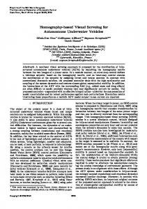
After detecting the end of a crop row, the row change behaviour is performed. In this behaviour, After detecting end of amanoeuvres crop row, the row change behaviour is performed. In row this to the robot performs thethe necessary to position itself at the head of the next behaviour, the robot performs the necessary manoeuvres to position itself at the head of the next row be inspected. This set of manoeuvres consists of a combination of straight-line and circular-arc to be inspected. This set of manoeuvres consists of a combination of straight-line and circular-arc movements with the help of the on board GPS. Specifically, it is a sequence of the following five moves movements with the help of the on board GPS. Specifically, it is a sequence of the following five (Figure 14): (1) straight-line forward movement to position itself outside the crop, in the header of the moves (Figure 14): (1) straight-line forward movement to position itself outside the crop, in the crop, to avoid crushing the crop in subsequent manoeuvres; (2) circular-arc movement towards the header of the crop, to avoid crushing the crop in subsequent manoeuvres; (2) circular-arc movement corresponding side of the next crop row to be inspected to position itself perpendicular to the crop towards the corresponding side of the next crop row to be inspected to position itself perpendicular rows; (3) straight-line movement; reverse circular-arc movement movement away fromaway the crop to the crop rows; (3)forward straight-line forward(4) movement; (4) reverse circular-arc fromrow to position itselftoparallel the direction the crop rows; and (5)rows; straight-line forward movement the crop row positiontoitself parallel toof the direction of the crop and (5) straight-line forward to place itself at the head of the next crop row to be inspected according to the plan. movement to place itself at the head of the next crop row to be inspected according to the plan.
Figure 14. Manoeuvres defined for crop row change.
Figure 14. Manoeuvres defined for crop row change.
3. Results and Discussion
3. Results and Discussion
To evaluate the performance and robustness of the proposed approach for central row To evaluate performance and were robustness of the proposed approach for central rowmode detection, detection, a setthe of 500 images, which acquired by the robot working in remote control in a set of 500 images, which acquired the robotdel working in remote control mode in different different maize fields andwere distinct days by at Arganda Rey (Madrid, Spain), were utilised. The maize fields andcaptured distinct in days at Arganda del Rey (Madrid, Spain), were utilised. imagesand were images were different conditions of illumination, growth stages, weedThe densities captured different conditions of illumination, stages, densities and camera orientations; camerain orientations; the robot operates in these growth conditions whenweed it autonomously navigates. Figure 15 severalinexamples of the employed theillustrates robot operates these conditions when itimages. autonomously navigates. Figure 15 illustrates several
examples of the employed images. The proposed approach was compared with a detection method that is based on the Hough transform [30], which is a strategy that was successfully integrated in some of our previous studies [36] in terms of effectiveness and processing time. The last aspect is really important in cases, such as this case, in which real-time detection is required. Both methods analysed the bottom half of each image, i.e., 1056 ˆ 352 pixels. The effectiveness was measured based on an expert criterion, in which the line that was detected was considered to be correct when it matched the real direction of the crop row. Table 4 shows the results from processing the 500 images with both approaches. The performance of the proposed approach exceeds the performance of a Hough-transform based strategy by 10%. The processing time that is required by the proposed approach is approximately four times less than the processing time required for the Hough transform, which indicates that the proposed approach can process approximately 14 frames in the best case compared with the Hough transform approach. The Hough transform approach can process three frames per second, which is less than the five frames per second that the EOS 7D camera provides (refer to Section 2 of this paper).
Sensors 2016, 16, 276
15 of 23
Sensors 2016, 16, 276
15 of 23
(a)
(b)
(c) Figure 15. (a)–(c) are examples of different images that were acquired by the camera of the robot. (a)
Figure 15. (a)–(c) are examples of different images that were acquired by the camera of the robot. shows the maize crops; (b) shows the crop rows where the irrigation system used is visible; (c) shows (a) shows the maize crops; (b) shows the crop rows where the irrigation system used is visible; (c) shows the kind of image to be taken when a crop border is being reaching . the kind of image to be taken when a crop border is being reaching. The proposed approach was compared with a detection method that is based on the Hough transform [30], which a strategy that was successfully of integrated in some of our previous Table 4. Detection of theiscentral crop row. Performance the proposed approach and an studies approach [36] in terms of effectiveness and processing time. The last aspect is really important in cases, such as that is based on the Hough transform.
this case, in which real-time detection is required. Both methods analysed the bottom half of each image, i.e., 1056 × 352 pixels. The effectiveness was measured based on an expert criterion, in which Approach Effectiveness (%) Mean Processing Time (seconds) the line that was detected was considered to be correct when it matched the real direction of the crop Proposed 96.4 the 500 images with both approaches. 0.069 row. Tableapproach 4 shows the results from processing The Hough-transform-based approach 88.4the performance of a Hough-transform 0.258 based performance of the proposed approach exceeds strategy by 10%. The processing time that is required by the proposed approach is approximately four times less than the processing time required for the Hough transform, which indicates that the To proposed test the approach differentcan behaviours developed for the robot, a test environment was established. process approximately 14 frames in the best case compared with the Hough Sensors 2016, 16, 276 16 of 23 Green lines wereapproach. painted in anHough outside soil plane to simulate cropthree rows. Theper lines werewhich 30 m in length transform The transform approach can process frames second, is and spaced 70 cm apart, as illustrated in Figure 16a. To make the environment more realistic, less than the five frames per second that the EOS 7D camera provides (refer to Section 2 of this length and spaced 70 cm apart, as illustrated in Figure 16a. To make the environment more realistic,weeds paper). and sowing errors introduced the lines. weeds and were sowing errors were along introduced along the lines. Table 4. Detection of the central crop row. Performance of the proposed approach and an approach that is based on the Hough transform.
Approach Proposed approach Hough-transform-based approach
Effectiveness (%) 96.4 88.4
Mean Processing Time (seconds) 0.069 0.258
To test the different behaviours developed for the robot, a test environment was established. Green lines were painted in an outside soil plane to simulate crop rows. The lines were 30 m in
(a)
(b)
Figure 16. (a) First test environment. (b) Crop employed in the experiments.
Figure 16. (a) First test environment. (b) Crop employed in the experiments. In this test environment, several experiments were performed to verify the proper functioning of the three autonomous robot behaviours described above: tracking, detection of the end of the crop row and row change. During the experiments, the robot followed the lines without headings, detected the row end, and changed rows, continuing the inspection, without human intervention. Figure 17 shows the evolution of the linear and angular speeds of the robot during the inspection of a line and the position of the robot with respect to the line (offset and angle) extracted by the image algorithm. Table 5 shows the mean, standard deviation, minimum and maximum of the linear speed, angular speed, offset and angle. The robot adjusted its linear speed depending on the error in
Sensors 2016, 16, 276
16 of 23
In this test environment, several experiments were performed to verify the proper functioning of the three autonomous robot behaviours described above: tracking, detection of the end of the crop row and row change. During the experiments, the robot followed the lines without headings, detected the row end, and changed rows, continuing the inspection, without human intervention. Figure 17 shows the evolution of the linear and angular speeds of the robot during the inspection of a line and the position of the robot with respect to the line (offset and angle) extracted by the image algorithm. Table 5 shows the mean, standard deviation, minimum and maximum of the linear speed, angular speed, offset and angle. The robot adjusted its linear speed depending on the error in its position; the speed was highest when the error in its position was 0 and decreased as the error increased, confirming the proper operation of the fuzzy controller of the linear speed. Variations in the angular speed were minimal because the error in the position was very small (offset and angle). The slight corrections to the left in the angular speed (negative values) were due to the tendency of the robot to veer towards the rightSensors when forward in its working operation (remote control mode). The design of the 2016,moving 16, 276 17 of 23 controller allowed these corrections to be made softly and imperceptibly during robot navigation and the necessary manoeuvres to change rows (Figure 19) to continue the inspection without human yielded movement in a straight line, which is impossible in remote control mode. intervention.
(a)
(b)
(c)
(d)
Figure 17. First test environment: (a) Evolution of the linear speed of the robot. (b) Evolution of the
Figure 17. First test environment: (a) Evolution of the linear speed of the robot. (b) Evolution of the angular speed of the robot. (c) Evolution of the offset of the robot relative to the line. (d) Evolution of angularthe speed robot. (c) Evolution angleof of the the robot relative to the line. of the offset of the robot relative to the line. (d) Evolution of the angle of the robot relative to the line.
Table 5. Results obtained in the test environment. Test environment
Mean
Std. dev.
Minimum
Maximum
Linear speed (cm/s) Angular speed (˝ /s) Offset (cm) (a) Angle (˝ )
28.66 ´0.57 0.55 0.52
0.68 0.53 0.47 0.38
26.20 ´2.00 (b) ´0.78 ´0.56
30.00 0.00 1.88 1.51
After confirming the performance of the robot in the test environment, several experiments were conducted in a real field at Arganda del Rey (Madrid, Spain). The field was a cereal field with crop row
(c)
(d)
Figure 18. Crop row tracking behaviour. Images from (a) to (d) show a sequence of different frames of the video available in [65].
(a)
(b)
Sensors 2016, 16, 276
17 of 23
spacing of 70 cm, which resembles a maize sowing schema. The rows were not perfectly straight and were characterised by strong high weed presence, as illustrated in Figure 16b. The robot was tested (c) the entire field. In this environment, (d) in different crop rows that covered the robot again followed the Figure 17. First testthe environment: (a) Evolution of the linear speedthe of the robot.end, (b) Evolution of the crop rows without crushing crops (Figure 18), detected row and performed the necessary angular speed of the robot. (c) Evolution of the offset of the robot relative to the line. (d) Evolution of manoeuvres to change rows (Figure 19) to continue the inspection without human intervention. the angle of the robot relative to the line.
(a)
(b)
(c)
(d)
Figure 18. Crop row tracking behaviour. Images from (a) to (d) show a sequence of different frames
Figure 18. Crop Images from (a) to (d) show a sequence of different frames of of therow videotracking available inbehaviour. [65]. the video available in [65]. Sensors 2016, 16, 276
18 of 23
(a)
(b)
(c)
(d)
(e) Figure 19. Sequence of manoeuvres performed by the robot to change rows. (a) corresponds with Figure 19. Sequence of 1manoeuvres performed by forward the robot to change rows. (a) corresponds with manoeuvre in Figure 14, i.e., the straight-line movement; (b) with the circular-arc manoeuvre (c) with straight-line forwardmovement; movement, manoeuvre 3; (d) reverse manoeuvre 1 inmovement, Figure 14, i.e., the2; straight-line forward (b) with thewith circular-arc movement, circular-arc movement, manoeuvre 4; (e) with straight-line forward movement, manoeuvre 5. Video manoeuvre 2; (c) with straight-line forward movement, manoeuvre 3; (d) with reverse circular-arc can be found in [65].
movement, manoeuvre 4; (e) with straight-line forward movement, manoeuvre 5. Video can be found However, the crop row tracking performance was worse in the real environment compared to in [65]. the first test environment. Figure 20 shows the evolution of the linear and angular speeds of the robot during the inspection of a line and the position of the robot with respect to the line (offset and angle) extracted by the image algorithm. Table 6 presents the values (mean, standard deviation, minimum and maximum) obtained for linear speed, angular speed, offset and angle. The difference in performance relative to the first environment is evident. The results were a consequence of the estimated position of the robot relative to the crop row (offset and angle). The image-processing algorithm correctly extracted the straight line defining the crop row. In contrast to the first test environment, the rows were not perfectly straight, which affected the performance of the robot. However, the difference in performance between the environments was primarily due to the
Sensors 2016, 16, 276
18 of 23
However, the crop row tracking performance was worse in the real environment compared to the first test environment. Figure 20 shows the evolution of the linear and angular speeds of the robot during the inspection of a line and the position of the robot with respect to the line (offset and angle) extracted by the image algorithm. Table 6 presents the values (mean, standard deviation, minimum and maximum) obtained for linear speed, angular speed, offset and angle. The difference in performance Sensors 2016, 16, 276 19 of 23 relative to the first environment is evident. The results were a consequence of the estimated position of the robot relative to the crop Table row (offset and angle). image-processing algorithm correctly 6. Results obtained in aThe real field. extracted the straight line defining the crop row. In contrast to the first test environment, the rows Realstraight, Field which affected Mean the performance Std. dev. of the Minimum Maximum were not perfectly robot. However, the difference in performance between the environments was primarily due to the differences between Linear speed (cm/s) 18.87 6.16 10.04 29.94the flat soil of the first environment and the abrupt soil of the field. The irregularities and roughness of the field, Angular (°/s) of the robot, −0.14 and the features 6.40 of the vehicle, −9.60 which did9.60 which hindered thespeed movement not provide any damping, caused vibrations and swinging in the pitch, yaw and roll angles of the camera during robot Offset (cm) 0.05 soil. These7.33 −14.00 16.00 navigation, particularly on the most rugged effects increased the variation in the estimated position of the robot as it moved in the field, which decreased the performance of the robot, slowed Angle (°) 0.53 3.32 −9.00 11.00 row tracking, and induced headings in stretches where the wheels of the robot had poor traction.
(a)
(c)
(b)
(d)
Figure Testsinina areal realfield: field: (a) (a) Evolution Evolution of (b)(b) Evolution of the Figure 20.20.Tests of the the linear linearspeed speedofofthe therobot. robot. Evolution of the angular speed of the robot. (c) Evolution of the offset of the robot relative to the line. (d) Evolution of of angular speed of the robot. (c) Evolution of the offset of the robot relative to the line. (d) Evolution the angle of the robot relative to the line. the angle of the robot relative to the line.
The observed variations are one of the challenges of using small field inspection vehicles Table 6. Results obtained in a real field. instead of tractors or large machines; for the latter, the displacement is more uniform, with fewer vibrations and variations in the camera. As observed in the experiments, although the robot was able Real Field Mean Std. dev. Minimum Maximum to navigate along the crop rows without crushing them, to improve its performance, the mechanical Linear speedmust (cm/s) 18.87or a more suitable 6.16 vehicle must 10.04be adopted 29.94 features of the robot be improved, to navigate the Angular speed (˝ /s) ´0.14 6.40 ´9.60 9.60 crop field. Note that the proposed navigation system can be easily adapted to control other types of Offset (cm) 0.05 7.33 ´14.00 16.00 vehicles as it isAngle based(˝on the vehicle model. ) driver behaviour 0.53 rather than3.32 ´9.00 11.00 4. Conclusions Crop inspection is a very important task in agriculture and PA, particularly when information about weed distribution is essential for generating proper risk maps that aid in site-specific treatment tasks. Among the various means of collecting field information, the use of small,
Sensors 2016, 16, 276
19 of 23
The observed variations are one of the challenges of using small field inspection vehicles instead of tractors or large machines; for the latter, the displacement is more uniform, with fewer vibrations and variations in the camera. As observed in the experiments, although the robot was able to navigate along the crop rows without crushing them, to improve its performance, the mechanical features of the robot must be improved, or a more suitable vehicle must be adopted to navigate the crop field. Note that the proposed navigation system can be easily adapted to control other types of vehicles as it is based on driver behaviour rather than the vehicle model. 4. Conclusions Crop inspection is a very important task in agriculture and PA, particularly when information about weed distribution is essential for generating proper risk maps that aid in site-specific treatment tasks. Among the various means of collecting field information, the use of small, autonomous vehicles with on-board sensing elements to minimise the impact on crop and soil compaction is quite promising. An autonomous field inspection vehicle, which autonomously navigates by visually tracking crop rows and following a previously established plan that guarantees the entire coverage of a field, was presented in this study. A set of basic behaviours necessary for an autonomous mobile robot to inspect a crop field with full coverage was established and implemented, including the tracking of a crop row, the detection of the end of a crop row, and the correct positioning of the robot at the head of the next row. An image-processing method capable of extracting the central crop row in the presence of weeds under uncontrolled lighting conditions in real time from images acquired with a reflex camera positioned at the front of the robot was developed. Two fuzzy controllers were also designed to achieve visual servoing for robot navigation. A method for detecting the end of the crop row using the images acquired by the camera was developed. In addition, the manoeuvres required to change rows were implemented. Several experiments were conducted to test the performance of the proposed and developed behaviours. These behaviours were performed in a test environment with plane soil. The robot was able to follow the lines, detect the row end, and change lines to continue the inspection without human intervention. The good results are due to the very small errors in the estimated position of the robot relative to the crop row. After these tests, a set of trials was performed on a real crop field. The robot was able to perform its behaviours correctly, although with reduced performance compared to the first test environment. This decreased performance is due to the variations in the estimated position of the robot relative to the crop row. The irregularities and roughness of the field hindered the movement of the robot, which lacked damping features, resulting in camera vibrations and swinging in its pitch, yaw and roll angles during robot navigation, particularly in the most rugged soil. These effects slowed the tracking of the crop row and induced headings in some areas where the wheels of the robot had poor traction. These variations were the main disadvantage we encountered when working with this small vehicle in the field. To improve the performance of the developed behaviours, the mechanical features of the robot should be modified, or an alternative vehicle better suited to navigating a crop field should be adopted. In the latter case, the approaches that are proposed in this paper can be integrated in the new vehicle just adapting slightly the value ranges of the fuzzy sets of the navigation control to the new vehicle. Acknowledgments: The Spanish Government has provided full and continuing support for this research work through projects AGL2011-30442-C02–02 and AGL2014-52465-C4-3-R. The authors wish to thank Pedro Hernáiz and his team (ICA-CSIC) for their invaluable help in the field trials. The authors wish to acknowledge the invaluable technical support of Damian Rodriguez. Author Contributions: The work was developed as a collaboration among all authors. J.M. Bengochea-Guevara and A Ribeiro designed the study. J.M. Bengochea-Guevara carried out the system integration and programming. D. Andújar posed the field experiments. J. Conesa-Muñoz mainly contributed to the development of the planner and provided support in the field tests with D. Andújar. A. Ribeiro directed the research, collaborating in the
Sensors 2016, 16, 276
20 of 23
testing and the discussion of the results. The manuscript was mainly drafted by J.M. Bengochea-Guevara and A. Ribeiro and was revised and corrected by all co-authors. All authors have read and approved the final manuscript. Conflicts of Interest: The authors declare no conflicts of interest.
Abbreviations The following abbreviations are used in this manuscript: CVRP DSS FOG GIS GNSS IMU PA PID RTK ExG b d g min_proportion r α D1 : D2
Capacited Vehicle Routing Problem Decision Support System Fibre Optic Gyroscope Geographical Information System Global Navigation Satellite System Inertial Measurement Unit Precision Agriculture Proportional Integral Derivative Real Time Kinematic Excess green index coefficient of the blue plane distance coefficient of the green plane Percentage threshold coefficient of the red plane motion direction angle Lower distance threshold Upper distance threshold
References 1. 2. 3. 4. 5. 6. 7. 8. 9. 10. 11.
Gebbers, R.; Adamchuk, V.I. Precision agriculture and food security. Science 2010, 327, 828–831. [CrossRef] [PubMed] Srinivasan, A. Handbook of Precision Agriculture: Principles and Applications; Food Products Press: New York, NY, USA, 2006. Stafford, J.V. Implementing precision agriculture in the 21st century. J. Agric. Eng. Res. 2000, 76, 267–275. [CrossRef] Reid, J.F. The impact of mechanization on agriculture. Bridge Agric. Inf. Technol. 2011, 41, 22–29. Senay, G.B.; Ward, A.D.; Lyon, J.G.; Fausey, N.R.; Nokes, S.E. Manipulation of high spatial resolution aircraft remote sensing data for use in site-specific farming. Trans. ASAE 1998, 41, 489–495. [CrossRef] Rew, L.J.; Cousens, R.D. Spatial distribution of weeds in arable crops: are current sampling and analytical methods appropriate? Weed Res. 2001, 41, 1–18. [CrossRef] Marshall, E.J.P. Field-scale estimates of grass weed populations in arable land. Weed Res. 1988, 28, 191–198. [CrossRef] Slaughter, D.C.; Giles, D.K.; Downey, D. Autonomous robotic weed control systems: A review. Comput. Electron. Agric. 2008, 61, 63–78. [CrossRef] Li, M.; Imou, K.; Wakabayashi, K.; Yokoyama, S. Review of research on agricultural vehicle autonomous guidance. Int. J. Agric. Biol. Eng. 2009, 2, 1–16. Stoll, A.; Kutzbach, H.D. Guidance of a forage harvester with GPS. Precis. Agric. 2000, 2, 281–291. [CrossRef] Blackmore, B.S.; Griepentrog, H.W.; Nielsen, H.; Nørremark, M.; Resting-Jeppesen, J. Development of a deterministic autonomous tractor. In Proceedings of the 2004 CIGR Olympics of Agricultural Engineering, Beijing, China, 11–14 October 2004.
Sensors 2016, 16, 276
12. 13. 14. 15.
16. 17. 18. 19. 20. 21. 22. 23. 24. 25. 26. 27.
28. 29. 30. 31. 32. 33. 34. 35.
36. 37.
21 of 23
Gomez-Gil, J.; Alonso-Garcia, S.; Gómez-Gil, F.J.; Stombaugh, T. A simple method to improve autonomous GPS positioning for tractors. Sensors 2011, 11, 5630–5644. [CrossRef] [PubMed] Alonso-Garcia, S.; Gomez-Gil, J.; Arribas, J.I. Evaluation of the use of low-cost GPS receivers in the autonomous guidance of agricultural tractors. Spanish J. Agric. Res. 2011, 9, 377–388. [CrossRef] Eaton, R.; Katupitiya, J.; Siew, K.W.; Howarth, B. Autonomous farming: Modelling and control of agricultural machinery in a unified framework. Int. J. Intel. Syst. Technol. Appl. 2010, 8, 444–457. [CrossRef] Kise, M.; Noguchi, N.; Ishii, K.; Terao, H. The development of the autonomous tractor with steering controller applied by optimal control. In Proceeding of the 2002 Automation Technology for Off-Road Equipment, Chicago, IL, USA, 26–27 July 2002; pp. 367–373. Nagasaka, Y.; Umeda, N.; Kanetai, Y.; Taniwaki, K.; Sasaki, Y. Autonomous guidance for rice transplanting using global positioning and gyroscopes. Comput. Electron. Agric. 2004, 43, 223–234. [CrossRef] Noguchi, N.; Kise, M.; Ishii, K.; Terao, H. Field automation using robot tractor. In Proceeding of the 2002 Automation Technology for Off-Road Equipment, Chicago, IL, USA, 26–27 July 2002; pp. 239–245. Bak, T.; Jakobsen, H. Agricultural robotic platform with four wheel steering for weed detection. Biosyst. Eng. 2004, 87, 125–136. [CrossRef] Marchant, J.A.; Hague, T.; Tillett, N.D. Row-following accuracy of an autonomous vision-guided agricultural vehicle. Comput. Electron. Agric. 1997, 16, 165–175. [CrossRef] Billingsley, J.; Schoenfisch, M. The successful development of a vision guidance system for agriculture. Comput. Electron. Agric. 1997, 16, 147–163. [CrossRef] Slaughter, D.C.; Chen, P.; Curley, R.G. Vision guided precision cultivation. Precis. Agric. 1999, 1, 199–217. [CrossRef] Tillett, N.D.; Hague, T. Computer-vision-based hoe guidance for cereals—An initial trial. J. Agric. Eng. Res. 1999, 74, 225–236. [CrossRef] Åstrand, B.; Baerveldt, A.-J. A vision based row-following system for agricultural field machinery. Mechatronics 2005, 15, 251–269. [CrossRef] Benson, E.R.; Reid, J.F.; Zhang, Q. Machine vision-based guidance system for agricultural grain harvesters using cut-edge detection. Biosyst. Eng. 2003, 86, 389–398. [CrossRef] Gottschalk, R.; Burgos-Artizzu, X.P.; Ribeiro, A.; Pajares, G. Real-time image processing for the guidance of a small agricultural field inspection vehicle. Int. J. Intel. Syst. Technol. Appl. 2010, 8, 434–443. [CrossRef] Kise, M.; Zhang, Q.; Rovira Más, F. A stereovision-based crop row detection method for tractor-automated guidance. Biosyst. Eng. 2005, 90, 357–367. [CrossRef] Sainz-Costa, N.; Ribeiro, A.; Burgos-Artizzu, X.P.; Guijarro, M.; Pajares, G. Mapping wide row crops with video sequences acquired from a tractor moving at treatment speed. Sensors 2011, 11, 7095–7109. [CrossRef] [PubMed] Søgaard, H.T.; Olsen, H.J. Determination of crop rows by image analysis without segmentation. Comput. Electron. Agric. 2003, 38, 141–158. [CrossRef] Hague, T.; Tillett, N.D.; Wheeler, H. Automated crop and weed monitoring in widely spaced cereals. Precis. Agric. 2006, 7, 21–32. [CrossRef] Hough, P.V. Method and Means for Recognizing Complex Patterns. US Patent US3069654 A, December 1962. Marchant, J.A. Tracking of row structure in three crops using image analysis. Comput. Electron. Agric. 1996, 15, 161–179. [CrossRef] Hague, T.; Marchant, J.A.; Tillett, D. A system for plant scale husbandry. Precis. Agric. 1997, 2, 635–642. Leemans, V.; Destain, M.-F. Application of the Hough transform for seed row localisation using machine vision. Biosyst. Eng. 2006, 94, 325–336. [CrossRef] Tellaeche, A.; Burgos-Artizzu, X.P.; Pajares, G.; Ribeiro, A. A vision-based method for weeds identification through the Bayesian decision theory. Pattern Recognit. 2008, 41, 521–530. [CrossRef] Tellaeche, A.; BurgosArtizzu, X.P.; Pajares, G.; Ribeiro, A.; Fernández-Quintanilla, C. A new vision-based approach to differential spraying in precision agriculture. Comput. Electron. Agric. 2008, 60, 144–155. [CrossRef] Tellaeche, A.; Pajares, G.; Burgos-Artizzu, X.P.; Ribeiro, A. A computer vision approach for weeds identification through Support Vector Machines. Appl. Soft Comput. 2011, 11, 908–915. [CrossRef] Kise, M.; Zhang, Q. Development of a stereovision sensing system for 3D crop row structure mapping and tractor guidance. Biosyst. Eng. 2008, 101, 191–198. [CrossRef]
Sensors 2016, 16, 276
38. 39.
40. 41. 42.
43. 44.
45. 46. 47. 48. 49.
50. 51.
52.
53.
54. 55.
56.
57. 58. 59.
22 of 23
Vioix, J.-B.; Douzals, J.-P.; Truchetet, F.; Assémat, L.; Guillemin, J.-P. Spatial and spectral methods for weed detection and localization. EURASIP J. Appl. Sign. Process. 2002, 2002, 679–685. [CrossRef] Bossu, J.; Gée, C.; Guillemin, J.P.; Truchetet, F. Development of methods based on double Hough transform and Gabor filtering to discriminate crop and weeds in agronomic images. In Proceedings of the SPIE 18th Annual Symposium Electronic Imaging Science and Technology, San Jose, CA, USA, 15–19 January 2006. Bossu, J.; Gée, C.; Jones, G.; Truchetet, F. Wavelet transform to discriminate between crop and weed in perspective agronomic images. Comput. Electron. Agric. 2009, 65, 133–143. [CrossRef] Romeo, J.; Pajares, G.; Montalvo, M.; Guerrero, J.M.; Guijarro, M.; Ribeiro, A. Crop row detection in maize fields inspired on the human visual perception. Sci. World J. 2012, 2012. [CrossRef] [PubMed] Conesa-Muñoz, J.; Gonzalez-de-Soto, M.; Gonzalez-de-Santos, P.; Ribeiro, A. Distributed multi-level supervision to effectively monitor the operations of a fleet of autonomous vehicles in agricultural tasks. Sensors 2015, 15, 5402–5428. [CrossRef] [PubMed] Bochtis, D.D.; Sørensen, C.G. The vehicle routing problem in field logistics part I. Biosyst. Eng. 2009, 104, 447–457. [CrossRef] Conesa-Munoz, J.; Bengochea-Guevara, J.M.; Andujar, D.; Ribeiro, A. Efficient Distribution of a Fleet of Heterogeneous Vehicles in Agriculture: A Practical Approach to Multi-path Planning. In Proceedings of the 2015 IEEE International Conference on Autonomous Robot Systems and Competitions (ICARSC), Vila Real, Portugal, 8–10 April 2015; pp. 56–61. Meyer, G.E.; Neto, J.C. Verification of color vegetation indices for automated crop imaging applications. Comput. Electron. Agric. 2008, 63, 282–293. [CrossRef] Woebbecke, D.M.; Meyer, G.E.; Von Bargen, K.; Mortensen, D.A. Color indices for weed identification under various soil, residue, and lighting conditions. Trans. ASAE 1995, 38, 259–269. [CrossRef] Andreasen, C.; Rudemo, M.; Sevestre, S. Assessment of weed density at an early stage by use of image processing. Weed Res. 1997, 37, 5–18. [CrossRef] Perez, A.J.; Lopez, F.; Benlloch, J.V.; Christensen, S. Colour and shape analysis techniques for weed detection in cereal fields. Comput. Electron. Agric. 2000, 25, 197–212. [CrossRef] Aitkenhead, M.J.; Dalgetty, I.A.; Mullins, C.E.; McDonald, A.J.S.; Strachan, N.J.C. Weed and crop discrimination using image analysis and artificial intelligence methods. Comput. Electron. Agric. 2003, 39, 157–171. [CrossRef] Yang, C.-C.; Prasher, S.O.; Landry, J.-A.; Ramaswamy, H.S. Development of an image processing system and a fuzzy algorithm for site-specific herbicide applications. Precis. Agric. 2003, 4, 5–18. [CrossRef] Ribeiro, A.; Fernández-Quintanilla, C.; Barroso, J.; García-Alegre, M.C.; Stafford, J.V. Development of an image analysis system for estimation of weed pressure. In Proceedings of 5th European Conference on Precision Agriculture, Uppsala, Sweden, 9–12 June 2005; pp. 169–174. Van Evert, F.K.; Van Der Heijden, G.W.; Lotz, L.A.; Polder, G.; Lamaker, A.; De Jong, A.; Kuyper, M.C.; Groendijk, E.J.; Neeteson, J.J.; Van der Zalm, T. A Mobile Field Robot with Vision-Based Detection of Volunteer Potato Plants in a Corn Crop. Weed Technol. 2006, 20, 853–861. [CrossRef] Burgos-Artizzu, X.P.; Ribeiro, A.; Tellaeche, A.; Pajares, G.; Fernández-Quintanilla, C. Analysis of natural images processing for the extraction of agricultural elements. Image Vision Comput. 2010, 28, 138–149. [CrossRef] Bengochea-Guevara, J.M.; Burgos Artizzu, X.P.; Ribeiro, A. Real-time image processing for crop/weed discrimination in wide-row crops. In Proceedings of RHEA, Madrid, Spain, 21–23 May 2014; pp. 477–488. Sheikholeslam, S.; Desoer, C. Design of decentralized adaptive controllers for a class of interconnected nonlinear dynamical systems. In Proceedings of the 31st IEEE Conference on Decision and Control, Tucson, AZ, USA, 16–18 December 1992; pp. 284–288. Rossetter, E.J.; Gerdes, J.C. Performance guarantees for hazard based lateral vehicle control. In Proceedings of the ASME 2002 International Mechanical Engineering Congress and Exposition, New Orleans, LA, USA, 17–22 November 2002; pp. 731–738. Pomerleau, D.A. Alvinn: An Autonomous Land Vehicle in a Neural Network; Technical Report CMU-CS-89–107; Carnegie Mellon University: Pittsburgh, PA, USA, 1989. Sugeno, M. On stability of fuzzy systems expressed by fuzzy rules with singleton consequents. IEEE Trans. Fuzzy Syst. 1999, 7, 201–224. [CrossRef] Zadeh, L.A. Fuzzy sets. Inf. Control 1965, 8, 338–353. [CrossRef]
Sensors 2016, 16, 276
60. 61. 62. 63. 64. 65.
23 of 23
Fraichard, T.; Garnier, P. Fuzzy control to drive car-like vehicles. Rob. Autom. Syst. 2001, 34, 1–22. [CrossRef] Naranjo, J.E.; Sotelo, M.; Gonzalez, C.; Garcia, R.; Sotelo, M.A. Using fuzzy logic in automated vehicle control. IEEE Intell. Syst. 2007, 22, 36–45. [CrossRef] Pradhan, S.K.; Parhi, D.R.; Panda, A.K. Fuzzy logic techniques for navigation of several mobile robots. Appl. Soft Comput. 2009, 9, 290–304. [CrossRef] Kodagoda, K.R.S.; Wijesoma, W.S.; Teoh, E.K. Fuzzy speed and steering control of an AGV. IEEE Trans. Control Syst. Technol. 2002, 10, 112–120. [CrossRef] Antonelli, G.; Chiaverini, S.; Fusco, G. A fuzzy-logic-based approach for mobile robot path tracking. IEEE Trans. Fuzzy Syst. 2007, 15, 211–221. [CrossRef] Digital.CSIC. Avalaible online: http://digital.csic.es/handle/10261/110162 (accessed on 11 December 2015). © 2016 by the authors; licensee MDPI, Basel, Switzerland. This article is an open access article distributed under the terms and conditions of the Creative Commons by Attribution (CC-BY) license (http://creativecommons.org/licenses/by/4.0/).